
10 VII July 2022 https://doi.org/10.22214/ijraset.2022.46093

Snehal B Kale1, Dr. Veena A. Shinde2, Dr. Vijay S. Koshti3 1, 2Department of Chemical of Engineering (of Affiliation) Bharati Vidyapeet Pune. MS India 3Department of Chemistry, D. P. Bhosale College Koregaon, Dist. Satara, MH 415501 Shivaji University KolhapurMS India
Coal is the most abundant and commonly used fossil fuel on the planet. It is a global industry that contributes significantly to global economic growth. Coal is mined commercially in more than 50 nations and used in more than 70. Annual global coal usage is estimated to be at 5,800 million tonnes, roughly 75% of that utilized to generate electricity. To meet the challenge of sustainable development and rising energy demand, this consumption is expected to double by 2030 nearly Coal is an explosive, lightweight organic origin rock that is black or dark brown and consists primarily of carbonized plant debris. It is found primarily in underground deposits with ash forming minerals [1]. With each passing year, the world's energy consumption grows. At this moment, fossil based fuels such as fuel oil, natural gas, and coal are used to meet most of the world's energy needs [2].Coal is one of the most widely used fossil fuels among various energy supplier materials due to its high carbon content. It is the most abundant and has the most extended life cycle, making it the most vital energy source in the long run. As a result, coal's most prominent application is in generating electricity in thermal power plants. On the other hand, coal can be used in a variety of industries for a variety of purposes, including cement manufacture, coke production for metallurgical furnaces, and household heating, depending on its rank (coal grade). Coal analysis can estimate the utility of coal in various sectors. "HyperCoal" (HPC) refers to ashless coal obtained using thermal solvent extraction. As inert chemical molecules and mineral debris are eliminated, HPC exhibits excellent fluidity [3]. HPC can be used in various applications, such as a fuel for low temperature catalytic gasification and as a replacement for caking coals [4,5]. Coal characteristics can be determined using processes outlined in internationally accepted test standards. Two test sets are used to determine the quality of coal: proximal and ultimate analysis.Moisture, ash, volatile matter, fixed carbon, and calorific values are measured in proximate analysis. Carbon, hydrogen, nitrogen, sulphur, and oxygen contents, on the other hand, are assessed in final analyses [4, 9]. However, the calorific value of coal is the most essential of them all.Estimating the coal's Gross CalorificValue (GCV) is crucial. Hence, the use of linear regression analysis to predict calorific value was examined. Finally, the MLRmodel was used to predict calorific value II. LITERATURESURVEY
International Journal for Research in Applied Science & Engineering Technology (IJRASET) ISSN: 2321 9653; IC Value: 45.98; SJ Impact Factor: 7.538 Volume 10 Issue VII July 2022 Available at www.ijraset.com 4960©IJRASET: All Rights are Reserved | SJ Impact Factor 7.538 | ISRA Journal Impact Factor 7.894 |
2) Mathematics is a concise language with well defined rules for manipulations.
A. What Is Mathematical Modeling Models describe our beliefs about how the world functions. In mathematical modeling, we translate those beliefs into the language of mathematics. This has many advantages
This section presents the different methodologies for the Prediction of Gross Calorific Value of coal.
1) Mathematics is an exact language. It helps us to formulate ideas and identify underlying assumptions.
Prediction of Gross Calorific Value of Coal using Machine Learning Algorithm
Keywords: Coal, RBFNN, GCV, GRNN, Machine learning, ML, SVM. I. INTRODUCTION
Abstract: The rising number of occurrences of coal grade slippage among coal suppliers and users is causing worry in the Indian coal industry.One of the most important metrics for determining coal quality is the Gross Calorific Value (GCV). As a result, good GCV prediction is one of the essential techniques to boost heating value and coal output. This system aims to estimate the GCV of the coal samples from proximate and ultimate parameters of coal using machine learning regression algorithm: the Multiple Linear Regression (MLR) and Local Polynomial Regression (LPR). The performance of this system is evaluated using Coefficient of determination (R2), Root Mean Squared Error (RMSE), and Mean Absolute Error (MAE) parameters. The results of the proposed system in terms of RMSE, MAE, and R2 of the MLR and LPR are observed as 0.124, 0.119, 0.414, and 0.654, 0.547, and 0.414, respectively.


4) Computers can be used to perform numerical calculations. There is a significant element of compromise in mathematical modeling. The majority of interacting systems in the real world are far too complicated to model in their entirety. Hence the first level of compromise is identifying the essential parts of the system. These will be included in the model; the rest will be excluded. The second level of compromise concerns the amount of mathematical manipulation which is worthwhile. Although mathematics has the potential to prove general results, these results depend critically on the form of equations used. Small changes in the structure of equations may require enormous changes in mathematical methods. Using computers to handle the model equations may never lead to elegant results, but it is more robust against alterations.
A phenomenological model is a scientific model that describes the empirical relationship of phenomena to each other in a consistent way with fundamental theory but is not directly derived from theory. In other words, a phenomenological model is not derived from the first principles. A phenomenological model forgoes any attempt to explain why the variables interact the way they do and simply attempts to describe the relationship, assuming that the relationship extends past the measured values.
International Journal for Research in Applied Science & Engineering Technology (IJRASET) ISSN: 2321 9653; IC Value: 45.98; SJ Impact Factor: 7.538 Volume 10 Issue VII July 2022 Available at www.ijraset.com 4961©IJRASET: All Rights are Reserved | SJ Impact Factor 7.538 | ISRA Journal Impact Factor 7.894 |
2) Phenomenological models have been characterized as being completely independent of theories, though many phenomenological models while failing to be derivable from a theory, incorporate principles and laws associated with theories
Mathematical modeling can be used for several different reasons. How well any particular objective is achieved depends on the state of knowledge about a system and how well the modeling is done. Examples of the range of objectives are:
1) Regression analysis is sometimes used to create statistical models that serve as phenomenological models.
1) Developing scientific understanding throughthe quantitative expression of current knowledge of a system (as well as displaying what we know, this may also show up what we do not know); 2) test the effect of changes in a system; 3) aid decision making, including a) tactical decisions by managers; b) strategic decisions by planners.
Empirical modeling refers to any kind of (computer) modeling based on empirical observations rather than on mathematically describable relationships of the system modeled. Empiricalmodeling is a generic term for activities that create models by observation and experiment. Empirical Modelling (EM) refers to a specific variety of empirical Modelling constructed models following particular principles. Though the extent to which these principles can be applied to model building without computers is an exciting issue, there are at least two good reasons to consider Empirical Modelling in the first instance as computer based. Undoubtedly, computer technologies have had a transformative impact where the full exploitation of Empirical Modelling principles is Whatconcerned.ismore, the conception of Empirical Modelling has been closely associated with thinking about the role of the computer in model building. An empirical model operates on a simple semantic principle: the maker observes a close correspondence between the model's behavior and that of its referent. The crafting of this correspondence can be 'empirical' in a wide variety of senses: it may entail a trial and error process, may be based on a computational approximation to analytic formulae, it may be derived as a black box relation. That affords no insight into 'why it works.' Empirical Modelling is rooted in the vital principle of William James's radical empiricism, which postulates that all knowing is rooted in given in experience connections
C. What Is Phenomenological Modeling
B. What Is The Necessity Of Modeling
D. What Is Empirical Modeling
3) The results that mathematicians have proved over hundreds of years are at our disposal.
3) The liquid drops model of the atomic nucleus, for instance, portrays the nucleus as a liquid drop and describes it as having several properties (surface tension and charge, among others) originating in different theories (hydrodynamics and electrodynamics, respectively). Certain aspects of these theories though usually not the complete theory are then used to determine the nucleus's static and dynamical properties
Modifications for constraints" genetic algorithms" refer to the biological evolution of a genotype that has inspired their particular way of incorporating random influences into the optimization process That way consists in:
International Journal for Research in Applied Science & Engineering Technology (IJRASET) ISSN: 2321 9653; IC Value: 45.98; SJ Impact Factor: 7.538 Volume 10 Issue VII July 2022 Available at www.ijraset.com 4962©IJRASET: All Rights are Reserved | SJ Impact Factor 7.538 | ISRA Journal Impact Factor 7.894 |
6) To repair the infeasible offspring by modifying it so that all constraints get fulfilled. This again can discard information on some offspring close to that optimum. Therefore, various modifications of the repair approach have been proposed that give up full feasibility, but preserve some information on the original offspring, e.g., repairing only randomly selected offspring (with a prescribed probability) or using the original offspring together with the value of the objective function of its repaired version.
7) To add the feasibility/infeasibility as another objective function, thus transforming the constrained optimization task into a task of multiobjective optimization.
5) To modify the objective function by a superposition of a penalty for infeasibility. This works well if theoretical considerations allow an appropriate choice of the penalty function. On the other hand, suppose some heuristic penalty function is used. In that case, its values typically turn out to be either too small, allowing the optimization paths to stay forever outside the feasibility area, or too large, thus suppressing the information on the value of the objective function for infeasible offspring
Instead, it focuses solely on certain kinds of ANN that have proven fruitful in solving real problems and gives four detailed examples of applications: 1) fault detection 2) prediction of polymer quality 3) data rectification 4) modeling and control for those who want more information,
Traditional approaches to solving chemical engineering problems frequently have their limitations, such as in the Modelling of highly complex and nonlinear systems. Artificial neural networks (ANN) have proved to solve complex tasks in some practical applications that should be of interest to you as a chemical engineer. This paper is not a review of the extensive literature that has been published in the last decade on artificial neural networks, nor is it a general review of artificial neural networks.
The fuzzy Logic 'Fuzzy' word is equivalent to inaccurate, approximate, and imprecise meaning. Fuzzy logic is a form of approximate reasoning rather than fixed or exact. Traditional binary sets have a truth value as either 0 or 1,which is true or false, while fuzzy logic has the truth value ranging between 0 and 1 Its truth value can take any magnitude range between 0 and 1 or true or false.Fuzzy logic emulates human reasoning and logical thinking systematically and mathematically.
3) Selecting the points for crossover and mutation according to a probability distribution is either uniform or skewed towards points where the objective function takes high values (the latter being a probabilistic expression of the survival of the fittest Inprinciple).thesearch for optimal catalysts in chemical engineering, it is helpful to differentiate between quantitative mutation, which modifies merely the proportionsof substances already present in the catalytic material, and qualitative mutation, which enters new substances or removes present ones (Figure 1). Genetic algorithms have been initially introduced for unconstrained optimization. However, there have been repeated attempts to modify them for constraints.
8) To modify the recombination and mutation operator to get closed concerning the set of feasible solutions. Hence, a mutation of a point that fulfills all the constraints or a recombination of two such points has to fulfill them.
F. Genetic Programming
1) randomly exchanging coordinates between two particular points in the input space of the objective function (recombination, crossover), 2) randomly modifying coordinates of a particular point in the input space of the objective function (mutation),
4) To ignore offspring's infeasible concerning constraints and not include them in the new population. Because in constrained optimization, the global optimum frequently lies on a boundary determined by the constraints. Ignoring infeasible offspring may discharge information on offspring very close to that optimum. Moreover, for some genetic algorithms, this approach can lead to the deadlock of not being able to find a whole population of viable offspring
G. Fuzzy Logic Controller
It provides an intuitive or perspective way to implement decision making, diagnosis, and control system implementation
E. Artificial Neural Network
H. Support Vector Regression
Fuzzy Logic controller structure Fuzzy logic controller is based on expert knowledge which provides means to convert the strategy for linguistic variable control into strategy for automatic control.
Mustafa Acikkar et al. [10] show how to use support vector machines (SVMs) and a feature selection approach to create new GCV, prediction models. To identify the relevance of each GCV predictor, the feature selector RReliefF is used to a dataset containing proximate and ultimate analytic variables. Seven separate hybrid input sets (data models) were created in this manner. The square of multiple correlation coefficient (R2), root mean square error (RMSE) and mean absolute percentage error (MAPE) was used to calculate the prediction performance of models.The predictor variables moisture (M) and ash (A) from the proximate analysis and carbon (C), hydrogen (H), and sulphur (S) from the ultimate analysis were found to be the most relevant variables in predicting coal GCV, while the predictor variables volatile matter (VM) from the proximate analysis and nitrogen (N) from the ultimate analysis had no positive effect on prediction accuracy. With 0.998, 0.22 MJ/kg, and 0.66 %, respectively, the SVM based model utilizing the predictor variables M, A, C, H, and S produced the best R squared value and the lowest RMSE and MAPE. GCV was also predicted using multilayer perceptron and radial basis function networks as a comparison.
1) Fuzzification: Fuzzification unit measures the real scalar values of variables inputted into the system. It then performs a scale mapping of the range of scalar values of input variables and then converts it to corresponding fuzzy value. Thus, fuzzification simply means converting the crisp input data into fuzzy value with help of suitable linguistic values and defined membership functions. Fuzzification process can be represented mathematically as given below: x = fuzzifier (x 0) Where x is the fuzzified value of the crisp input value.
The fuzzy logic controller encompasses four main components viz. Fuzzification unit, Fuzzy Knowledge Base, Decision making unit, and Defuzzification unit. These are explained briefly below.
Kernel based techniques (such as support vector machines, Bayes point machines, kernel principal component analysis, and Gaussian processes) represent a major development in machine learning algorithms. Support vector machines (SVM) are a group of supervised learning methods that can be applied to classification or regression. In a short period of time, SVM found numerous applications in chemistry, such as in drug design, quantitative structure activity relationships, chemometrics, sensors, chemical engineering, and text mining. Support vector machines represent an extension to nonlinear models of the generalized portrait algorithm developed by Vapnik and Lerner. A support vector machine (SVM) is machine learning algorithm that analyses data for classification and regression analysis. SVM is a supervised learning method that looks at data and sorts it into one of two categories. An SVM outputs a map of the sorted data with the margins between the two as far apart as possible. The basic idea of regression estimation is to approximate the functional relationship between a set of independent variables and a dependent variable by minimising a "risk" functional which is a measure of prediction errors.
I. State Of Art Approach For Prediction Of Gross Calorific Value Of Coal Using Machine Learning Algorithm
3) Decision Making Unit: The Decision making unit is the heart or kernel of a fuzzy logic controller which has the capability of inferring fuzzy control actions employing rules of inference in fuzzy logic. A set of IF THEN rules are used for inferring a control action based on expert knowledge or designing. IF (antecedents are satisfied) THEN (consequents are inferred) IF THEN rules are accompanied with linguistic variables and are frequently called as fuzzy conditional statements, or fuzzy controlled rules. IF THEN rules can be also be used with logic operators such as Boolean operators for applying multiple antecedents or multiple consequents.
Using traditional binary sets, it is not possible to precisely classify the color of the apples as completely dark i.e., 0 or false and completely lighter than the other i.e. 1 or true. Membership functions are user defined values for the linguistic variables. Thus, the human logic reasoning capabilities can be implemented for controlling complex real world systems.
4) Defuzzification: The last unit of the fuzzy logic controller is the defuzzification unit which converts a inferred fuzzy control value from the decision making unit to a non fuzzy or a crisp control value, which is fed to the process for the controlling action. In defuzzification a scale mapping is done to convert a fuzzy value to a non fuzzy value. Defuzzification can be done by various methods. The most used method is the Centre of Gravity method to get the most desired control value.
2) Fuzzy Knowledge Base: It consists of a database comprising of the necessary definitions used to describe linguistic variables and fuzzy data manipulation also it consists of a rule base comprising the control goals and control policy defined by the experts by means of linguistic control rules.
International Journal for Research in Applied Science & Engineering Technology (IJRASET) ISSN: 2321 9653; IC Value: 45.98; SJ Impact Factor: 7.538 Volume 10 Issue VII July 2022 Available at www.ijraset.com 4963©IJRASET: All Rights are Reserved | SJ Impact Factor 7.538 | ISRA Journal Impact Factor 7.894 |
J. Fu [12] describes the use of statistical models to quickly and accurately quantify GCV utilizing coal components with mensuration in real time online in China to fulfill practical demands. Researchers have developed linear regression (LM), nonlinear regression equation (NLM), and artificial neural networks (ANN) for estimating GCV. The GCV of China coal is predicted using 1400 data points in this paper. The support vector machine (SVM) is used to determine the progress of the estimating process, and the estimating robustness is assessed. The SVM model outperformed the three existing models in terms of accuracy and robustness, according to the comparative research. Meanwhile, the sampling process has been enhanced, and the number of input variables has been decreased to the absolute minimum. The prediction of calorific value was explored using linear regression analysis, including simple linear regression analysis and MLRanalysis, and prediction models were built, according to S. Yerel and T. Ersen [13]. Following that, statistical tests were used to verify the constructed models. A MLRmodel was shown to be reliable for estimating calorific values. For mining planning, the approach provides both practical and economic benefits Regression analysis, such as simple linear regression analysis and MLRanalysis, was used to analyzethe calorific value, ash content, and moisture content in this study. The multiple regression model was shown to be the best model in regression analysis. The multiple regression model's determination R2 is 89.2 percent. This is an excellent value that indicates the correct model. This finding demonstrates the utility of a MLRmodel for predicting calorific value. To manage the coal deposit, these models assess factors such as calorific value, ash concentration, and moisture content M. Sozer et al. [14] propose an MLR algorithm for coal GCV prediction. The predictive parameters' importance was investigated using R2, adj. R2, standard error, F values, and p values. MLR offered an acceptable correlation between HHV and any of the single parameters, although connections between HHV and any of the single parameters were almost irregular. In forecasting the HHV, it was also discovered that ultimate analysis parameters (C, H, and N) were more important than proximal analysis factors (fixed carbon (FC), volatile matter (VM), and ash). When elemental C content was present in the regression equation, FC content was considered as an inefficient parameter. The elemental C content became the most dominating parameter after proximal analysis parameters were removed from the equation, resulting in extremely low p values. For hardcoals, adj. R2 of the equation with three parameters (HHV = 87.801(C) + 132.207(H) − 77.929(S)) was slightly higher than that of HHV = 11.421(Ash) + 22.135(VM) + 19.154(FC) + 70.764(C) + 7.552(H) − 53.782(S). Yilmaz et al. [15], currently available The determination of coal's GCVis critical for characterizing coal and organic shales; yet, it is a complex, expensive, time consuming, and damaging process. The application of various artificial neural network learning techniques such as MLP, RBF (exact), RBF (k means), and RBF (SOM) for the prediction of GCV was reported in this research. As a consequence of this study, all models performed well in predicting GCV. Although the four different ANN algorithms have nearly identical prediction capabilities, MLP has greater accuracy than the other models. Soft computing techniques will be used to develop new ideas and procedures for predicting certain factors in fuel research. The input layer, the hidden layer, and the output layer make up an RBFNN, which is a feed forward neural network with three layers. In terms of node properties and learning algorithms, RBFNN is akin to a particular example of multilayer feed forward neural networks [16]. The outputs of Gaussian functions in the hidden layer neurons are inversely proportional to the distance from the neuron's center. RBFNNs and GRNNs are extremely comparable. The primary distinction is that in GRNN, one neuron is assigned to each point in the training file, but in RBFNN, the number of neurons is frequently significantly smaller than the number of training points [17] The RBFNN model's training phase determines four distinct parameters. The numbers of neurons in the hidden layer, the center coordinates of each RBF function in the hidden layer, the radius (spread) of each RBF function in each dimension, and the weights applied to the RBF function output as they are transmitted to the output layer are the parameters [17]
International Journal for Research in Applied Science & Engineering Technology (IJRASET) ISSN: 2321 9653; IC Value: 45.98; SJ Impact Factor: 7.538 Volume 10 Issue VII July 2022 Available at www.ijraset.com 4964©IJRASET: All Rights are Reserved | SJ Impact Factor 7.538 | ISRA Journal Impact Factor 7.894 | Bui et al. [11] developed the particle swarm optimization (PSO) support vector regression (SVR) model as a unique evolutionary based prediction system for forecasting GCV with good accuracy. The PSO SVR models were built using three different kernel functions: radial basis function, linear, and polynomial functions. In addition, three benchmark machine learning models were developed to estimate GCV, including Classification and Regression Tree (CART), MLR, and Principal Component Analysis (PCA), and then compared to the proposed PSO SVR model; 2583 coal samples were used to analyze the proximate components and GCV for this study.They were then utilized to create the aforementioned models and test their performance in experimental findings. The GCV prediction models were evaluated using RMSE, R2, ranking, and intensity color criteria. The suggested PSO SVR model with radial basis function exhibited superior accuracy than the other models, according to the findings. With excellent efficiency, the PSO method was improved in the SVR model. To assess the heating value of coal seams in difficult geological settings, they should be employed as a supporting tool in practical engineering.
International Journal for Research in Applied Science & Engineering Technology (IJRASET) ISSN: 2321 9653; IC Value: 45.98; SJ Impact Factor: 7.538 Volume 10 Issue VII July 2022 Available at www.ijraset.com 4965©IJRASET: All Rights are Reserved | SJ Impact Factor 7.538 | ISRA Journal Impact Factor 7.894 | III. ARTIFICIALNEURAL NETWORK
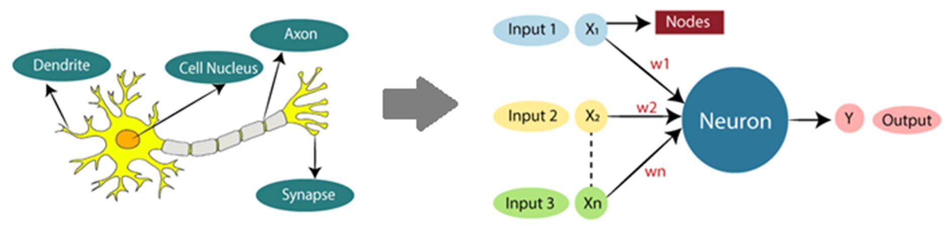
The term "Artificial Neural Network" is derived from Biological neural networks that develop the structure of a human brain. Similar to the human brain that has neurons interconnected to one another, artificial neural networks also have neurons that are interconnected to one another in various layers of the networks. These neurons are known as nodes.
2) Hidden Layer: The hidden layer presents in between input and output layers. It performs all the calculations to find hidden features and patterns.
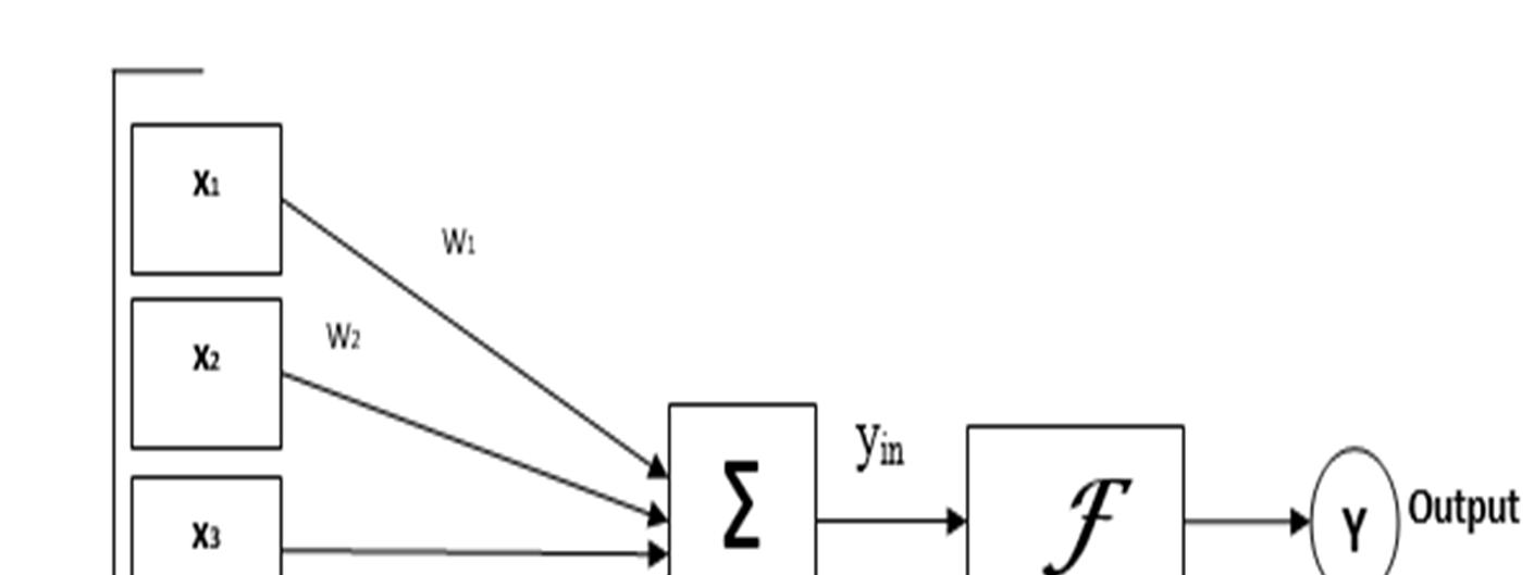
3) Output Layer: The input goes through a series of transformations using the hidden layer, which finally results in output that is conveyed using this layer.The artificial neural network takes input and computes the weighted sum of the inputs and includes a bias. This computation is represented in the form of a transfer function. ∑ ∗ + (1) It determines weighted total is passed as an input to an activation function to produce the output. Activation functions choose whether a node should fire or not. Only those who are fired make it to the output layer.
The architecture of the neural network consists of Input Hidden and output layer.
Dendrites from Biological Neural Network represent inputs in Artificial Neural Networks, cell nucleus represents Nodes, synapse represents Weights, and Axon represents Output.
The architecture of the neural network is givenFig.3.2.below.Architecture of artificial neural network
Fig.3.1. Relationship between Biological neural network and artificial neural network
1) Input Layer: As the name suggests, it accepts inputs in several different formats provided by the programmer.
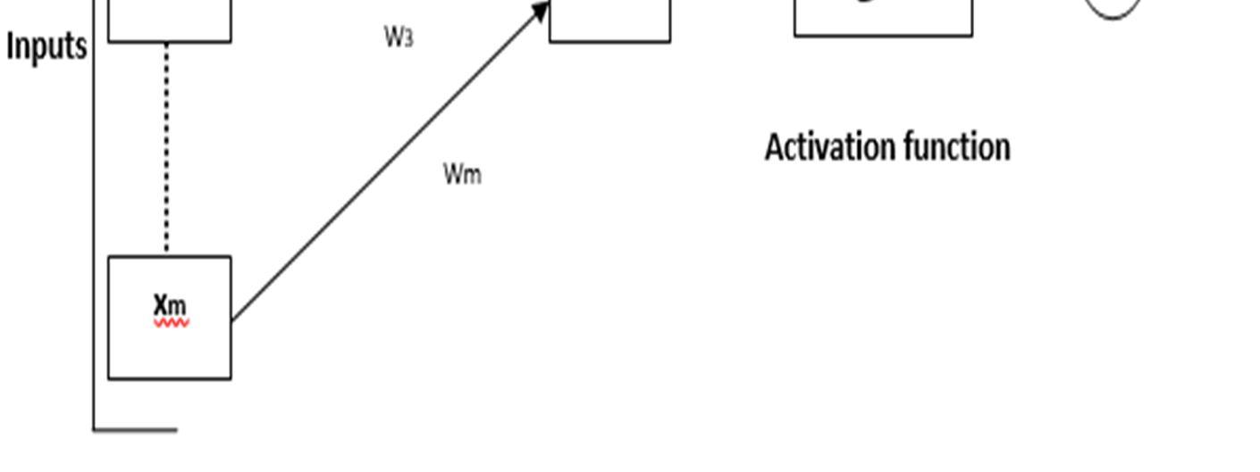
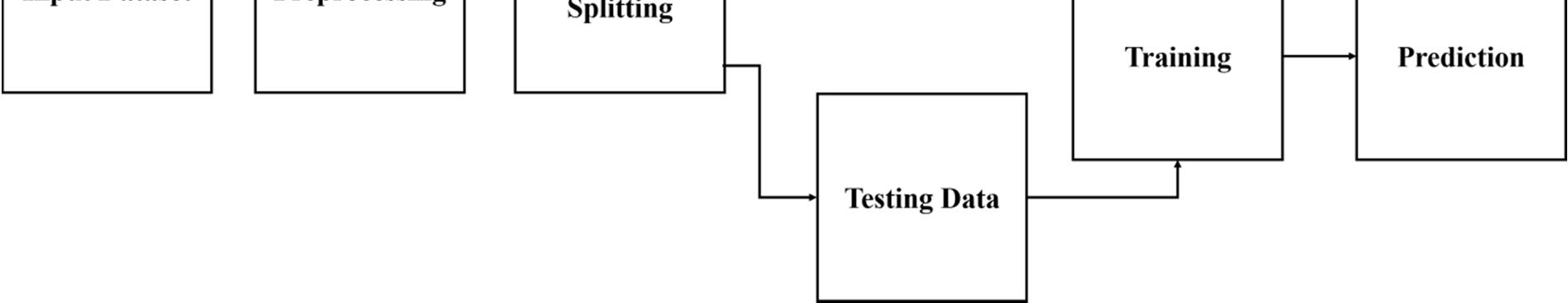
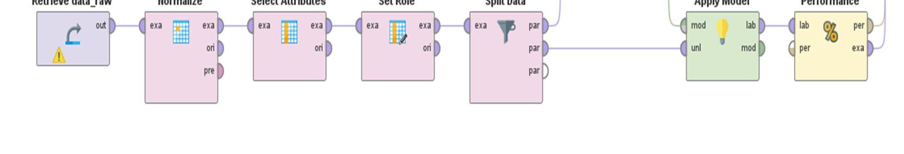
International Journal for Research in Applied Science & Engineering Technology (IJRASET) ISSN: 2321 9653; IC Value: 45.98; SJ Impact Factor: 7.538 Volume 10 Issue VII July 2022 Available at www.ijraset.com 4966©IJRASET: All Rights are Reserved | SJ Impact Factor 7.538 | ISRA Journal Impact Factor 7.894 | IV. PROPOSEDSYSTEM The Block diagram of the proposed system for prediction of GCV using machine learning regression technique is shown in Fig.3.1. Fig.1. Block diagram of the proposed system A detailed explanation of each block is discus is this section A. Input Dataset The dataset for the evaluation of the proposed system is taken from [18]. The properties of the coal sample are shown in Table 1. Table 1. Properties of Coal Samples (Kobe) ID Proximate Analysis Ultimate Analysis ExtractionYieldmoisture ash mattervolatile C H N S O 1 1.2 5 36.7 87.3 6 2 1.5 3.1 81.8 2 1.8 9.8 29.4 87.1 5.4 2.4 0.6 4.4 72.8 3 0.7 13.1 28.2 86.2 5.1 1.9 2.2 4.6 72.5 4 3.4 12.6 39.3 78.9 5.4 1.3 4.2 10.2 69.2 5 2.3 6 33.5 84.7 5.4 2.3 0.6 7.1 68.8 6 1.4 8.5 28 86.6 5.2 2.5 0.7 4.9 66.7 7 1.6 10.3 28.8 87 5.5 2.3 0.7 4.6 66.1 8 3.3 12.5 39.4 80.3 5.5 1.1 3.6 9.5 65.2 9 5.5 9.8 29.5 87.9 5.3 2.2 0.7 4 62.1 10 2.5 5.8 34 84.4 5.4 2.3 0.6 7.3 61.1 11 4.3 6.8 33.2 86 5.4 2.4 0.7 5.5 60.8 12 2.4 7.7 33.3 84.4 5.4 2.3 0.7 7.3 59.4 13 3.9 4.7 36.4 84 5.4 1.9 0.5 8.2 58.9 14 7.9 15.4 40.9 76.2 5.4 1.3 5.7 11.4 58.9 15 7.5 11.5 49 79.6 6.3 1.6 1 11.5 58.7 16 5.6 5.6 44.2 76.4 5.5 1.9 0.9 15.4 58 17 3.3 8.8 34.3 81.7 5.3 1.9 0.6 10.5 56.6 18 0.9 10 26.8 87.5 5.2 1.7 0.4 5.1 54.4 19 3.9 7.3 27.3 87.3 4.9 1.8 0.4 5.6 53.1 20 4.3 8.4 32.4 78.2 4.9 2.2 0.7 14 51.6 21 3.2 8.2 37.3 82.3 5.5 1.9 0.6 9.8 51.5 22 1.7 5 39 82.9 5.6 1.6 1 8.9 51.5
International Journal for Research in Applied Science & Engineering Technology (IJRASET) ISSN: 2321 9653; IC Value: 45.98; SJ Impact Factor: 7.538 Volume 10 Issue VII July 2022 Available at www.ijraset.com 4967©IJRASET: All Rights are Reserved | SJ Impact Factor 7.538 | ISRA Journal Impact Factor 7.894 | 23 3.8 8.4 36.6 83 5.4 2 0.6 9 51.4 24 3.6 5.9 35.4 83 5.6 1.9 0.4 9.1 51.1 25 5.5 9.2 35.9 84 5 1.5 0.7 8.8 50.7 26 2.1 8.6 34.1 84.5 5.3 1.5 0.3 8.4 48.4 27 1.5 3 46.8 79.2 5.9 1.2 3.4 10.3 48.2 28 6.3 4.8 42.7 78.7 5.6 1.7 0.6 13.3 47 29 4.5 8 34.5 82.8 5.2 1.9 0.5 9.6 46 30 5 10.8 23.3 78.7 4.2 1.4 1.1 14.6 45.9 31 7.1 15.4 44.5 60.8 4.7 1.7 6.8 25.9 45.5 32 8.7 6 44.2 76.7 5.6 1.9 0.9 15 45 33 24.7 3.2 55.1 69.5 5.5 0.9 0.3 23.8 45 34 25.3 10.6 47.1 72.1 5.4 1 0.3 21.1 44.4 35 2.2 11.2 32.6 83.6 5.2 1.6 0.6 9 43.9 36 3.3 8.4 36.3 82.5 5.1 1.6 0.5 10.4 43.4 37 14.8 8.8 44.5 71.9 5.6 1.6 1.9 19 43.2 38 1.7 11.9 48.3 68.9 5.8 1.1 0.3 23.8 42.9 39 4.8 8.5 19.8 90.7 4.5 1.5 1 2.3 42 40 6.2 9.4 26.5 87.9 4.7 2.1 0.5 4.7 40.3 41 6.8 7.1 32.1 83.8 4.2 1.9 0.6 9.6 40.1 42 33 1 51.8 70.5 5 1.1 0.1 23.2 39.8 43 36 7.2 50.5 68.4 4.9 1.2 0.2 25.3 39.3 44 11 1.9 49.2 69.3 4.8 1.3 0.7 23.9 38.8 45 3.3 15.2 34.4 82 5.4 2.5 0.4 9.7 38.2 46 15.5 11.9 42.1 74.6 5.8 1.8 0.6 17.1 38.2 47 2.5 17.4 34.1 82 5.3 1.6 1.1 10 38 48 17.2 24.9 35.6 76.1 5.5 2.2 1.1 15 38 19 7.7 17.3 36.6 77.7 5.2 1.2 0.3 15.7 37.1 50 5.1 13.8 38.3 68 4.6 1.3 0.5 25.6 36.7 51 1.7 4.2 53 69.9 5.3 1 0.2 23.6 36.2 52 2.6 11.6 38.5 81 5.4 1.7 0.9 10.9 36 53 2.6 11.6 38.5 71.6 4.8 1.5 0.8 21.3 36 54 30.3 2 47.8 67.4 4.8 1.1 0.2 26.5 35.4 55 1.5 3 32.6 82.2 5 2.2 0.6 10.1 35.2 56 26.2 1.7 72.4 72.4 5.1 1.6 0.6 20.4 34.8 57 3.3 13.7 30.8 72.5 4.2 1.6 0.5 21.2 33.8 58 4.3 11.4 38.4 77.9 5.4 2 1.3 13.3 33.7 59 6.1 6.6 36.2 76.7 4.9 1.8 0.4 16.2 33.3 60 3.8 11.5 34.6 70.9 4.4 1.3 0.7 22.6 32 61 10.2 6 31.9 78.2 4.7 1.4 1.1 14.6 31.2 62 11.4 4.8 40.5 74.5 4.4 1.7 0.3 19.1 30.6 63 2.1 9.5 17.7 90.6 4.5 1 0.2 3.7 30.2 64 3.8 5.5 40.8 71.7 4.9 1.9 1 20.5 29.6 65 2 6.9 29.9 79.5 4.4 0.7 0.7 14.8 28.2 67 3.8 10.2 32.2 84.3 4.7 2.1 0.6 8.3 26.9 68 1.5 4.5 46.9 76.3 5.6 1.4 0.4 16.3 26.6 69 8.4 8.3 32.3 74.8 4.3 1.8 0.4 18.8 24.6 70 10.1 4.2 51.6 70.3 5.3 1.3 1.5 21.6 24.3 71 12.2 9.2 42 76.8 5.5 1.2 0.2 16.3 24.1
2) Root Mean Squared Error (RMSE): The RMSE, also known as root mean square deviation, is one of the most extensively used methods for evaluating the validity of forecasts. It shows how much forecasts depart from measured true values using Euclidean distance. We get Root Mean Squared Error by taking the square root of the MSE (RMSE). RMSE is commonly used in supervised learning applications since it uses and requires real measurements at each predicted data point = ∑ ( ) (4) where N is the number of data points, y(i) is the ith measurement, and is its corresponding prediction.
International Journal for Research in Applied Science & Engineering Technology (IJRASET) ISSN: 2321 9653; IC Value: 45.98; SJ Impact Factor: 7.538 Volume 10 Issue VII July 2022 Available at www.ijraset.com 4968©IJRASET: All Rights are Reserved | SJ Impact Factor 7.538 | ISRA Journal Impact Factor 7.894 | 72 5 6.8 33 80.4 4.5 1 0.2 13.9 23.1 73 2.5 14.9 25.1 72 3.7 1.7 0.5 22.1 20.9 74 9.2 5.4 34 76.5 4.4 1 0.6 17.5 20.8 75 0.7 9.6 19 79.6 6.3 1.6 1 11.5 20.4
D. Model Training In this system, a MLRalgorithm is used to train and validate the input coal data. Multi linear regression is a mathematical strategy to determine a relationship between a group of independent variables (input values) and the dependent variables (GCV) (proximate and ultimate analysis parameter). Based on the input qualities indicated in the metadata column, this algorithm predicts the GCV. MLR is a statistical approach that uses a combination of explanatory factors to predict the outcome of a response variable. The MLR formula is as follows: = + + +⋯+ + (2) where, is the dependent variable, is the explanatory variables, =y intercept (constant term), is theslope coefficients for each explanatory variable, is the model's error term or residuals
E. Testing And Evaluation
C. Dataset Splitting
The machine learning algorithms need training as well as validation data to test the unknown data and evaluate the performance of the system. In this system, the whole dataset is divided into 80% data used for training and 20% data for validation.
1) Coefficient of determination (R2): The sum of squares of residuals (SSres) from the regression model is divided by the total sum of squares (SStot) of errors from the average model, then subtracted from 1. The Coefficient of Determination is another name for R squared. It illustrates how much variance in the output/predicted variable is explained by the input variables =1 1 ∑ ( ) ∑ ( ) (3)
The machine learning algorithm needs pre processed data to achieve high accuracy. In this system, normalization is used for pre processing. Normalization is a data preparation technique that is frequently used in machine learning. The process of transforming the columns in a dataset to the same scale is referred to as normalization. Every dataset does not need to be normalized for machine learning. It is only required when the ranges of characteristics are different. The most widely used types of normalization in machine learning are Min Max and Standardization scaling. Normalization in machine learning is the process of translating data into the range [0, 1]. The normalization is presented by Eq.(1). = (1) Here, and are the maximum and the minimum values of the feature respectively.
The performance of the system using Coefficient of determination (R2), Root Mean Squared Error (RMSE), Mean Absolute Error (MAE) parameters.
B. Preprocessing
The estimate of the extraction yield with 1 MN for 76 coals (Table 1) was performed using various analytical values. Table I consist of proximate and ultimate analysis parameter as input while the output parameter is extraction yield.
International Journal for Research in Applied Science & Engineering Technology (IJRASET) ISSN: 2321 9653; IC Value: 45.98; SJ Impact Factor: 7.538 Volume 10 Issue VII July 2022 Available at www.ijraset.com 4969©IJRASET: All Rights are Reserved | SJ Impact Factor 7.538 | ISRA Journal Impact Factor 7.894 | 3) Mean Absolute Error (MAE): The amount of the difference between the prediction of observation and the true value of that observation is referred to as the Absolute Error. The size of mistakes for a group of predictions and observations is measured using the average of absolute errors for the entire group. The L1 loss function is another name for MAE = ∑ | | (5) Where is the prediction and is the true value V. RESULTSANDDISCUSSION
The
Table 2. Normalized dataset ID Proximate Analysis Ultimate Analysis ExtractionYieldmoisture ash mattervolatile C H N S O 1 0.73507 0.88596 0.001936 1.265280 1.646587 0.776202 0.505235 1.51838 81.8 2 0.65584 0.26914 0.76566 1.234508 0.539148 1.70155 0.28556 1.32346 72.8 3 0.80109 1.063286 0.89184 1.096036 0.01457 0.54486 1.120304 1.29347 72.5 4 0.44458 0.942962 0.275328 0.02712 0.539148 0.84316 2.877645 0.45378 69.2 5 0.58982 0.64531 0.33454 0.865249 0.539148 1.470218 0.28556 0.91860 68.8 6 0.70866 0.04369 0.91287 1.157579 0.170001 1.932895 0.19770 1.24848 66.7
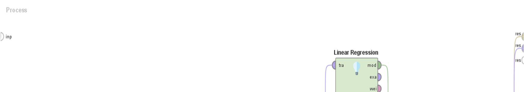
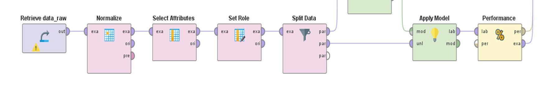
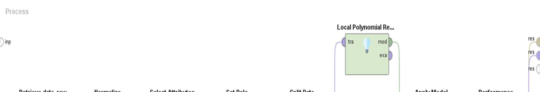
Fig.4.1.Process diagram of MLR for the proposed system diagram of LPRfor the proposed system input data is first preprocessed using thenormalization technique and it is tabulated in Table 2.
The results are implemented using the rapid minor platform on the Windows 10 operating system. The data is trained using a MLR algorithm and the performances in predicting GCV by using the validation data.Themodel architecture of the proposed multiple regression model on rapid Minor is as shown in Fig.4.1. while the process diagram of LPR is presented in Fig.4.2.
Fig.4.1.Process
International Journal for Research in Applied Science & Engineering Technology (IJRASET) ISSN: 2321 9653; IC Value: 45.98; SJ Impact Factor: 7.538 Volume 10 Issue VII July 2022 Available at www.ijraset.com 4970©IJRASET: All Rights are Reserved | SJ Impact Factor 7.538 | ISRA Journal Impact Factor 7.894 | 7 0.68225 0.389470 0.82875 1.219123 0.723721 1.470218 0.19770 1.29347 66.1 8 0.45779 0.918897 0.285843 0.188273 0.723721 1.30584 2.350443 .558741 65.2 9 0.16730 0.269146 0.75514 1.35759 0.35457 1.238879 0.19770 1.38343 62.1 10 0.56342 0.69344 0.28196 0.819092 0.539148 1.470218 0.28556 0.88862 61.1 11 0.32575 0.45279 0.36608 1.065264 0.539148 1.701557 0.19770 1.15852 60.8 12 0.57662 0.23621 0.35557 0.819092 0.539148 1.470218 0.19770 0.88862 59.4 13 0.37856 0.95816 0.02960 0.757548 0.539148 0.544863 0.37343 0.75366 58.9 14 0.149585 1.616778 0.443569 0.44254 0.539148 0.84316 4.195651 0.27384 58.9 15 0.096770 0.678249 1.295288 0.080573 2.200307 0.14915 0.065900 0.25885 58.7 16 0.15410 0.74157 0.790566 0.41177 0.723721 0.544863 0.02196 0.325932 58 17 0.45779 0.028497 0.25042 0.403675 0.354574 0.544863 0.28556 0.40879 56.6 18 0.77468 0.317276 1.03905 1.296052 0.170001 0.082186 0.46130 1.21849 54.4 19 0.37856 0.33247 0.98647 1.265280 0.38371 0.313524 0.46130 1.14352 53.1 20 0.32575 0.06776 0.45021 0.13482 0.38371 1.238879 0.19770 0.116009 51.6 21 0.47099 0.11589 0.065027 0.495989 0.723721 0.544863 0.28556 0.51375 51.5 22 0.66905 0.88596 0.243783 0.588304 0.908294 0.14915 0.065900 0.64870 51.5 23 0.39177 0.06776 0.00857 0.603690 0.539148 0.776202 0.28556 0.63371 51.4 24 0.41817 0.66938 0.13475 0.603690 0.908294 0.544863 0.46130 0.61871 51.1 25 0.16730 0.124757 0.08218 0.757548 0.19914 0.38049 0.19770 0.66370 50.7 26 0.61623 0.01963 0.27145 0.834477 0.354574 0.38049 0.54916 0.72368 48.4 27 0.69545 1.36726 1.063957 0.019029 1.462014 1.07450 2.174709 0.43878 48.2 28 0.06167 0.93409 0.632840 0.05789 0.908294 0.082186 0.28556 0.011048 47 29 0.29934 0.16402 0.22939 0.572919 0.170001 0.544863 0.37343 0.54374 46 30 0.23332 0.509795 1.40708 0.05789 1.67573 0.61183 0.153767 0.205976 45.9 31 0.043954 1.616778 0.822111 2.81195 0.75286 0.082186 5.162188 1.900353 45.5 32 0.255216 0.64531 0.790566 0.36561 0.908294 0.544863 0.02196 0.265954 45 33 2.367829 1.31913 1.936707 1.47339 0.723721 1.76852 0.54916 1.585469 45 34 2.447052 0.461665 1.095502 1.07336 0.539148 1.53718 0.54916 1.180618 44.4 35 0.60303 0.606054 0.42918 0.696005 0.170001 0.14915 0.28556 0.63371 43.9 36 0.45779 0.06776 0.04012 0.526761 0.01457 0.14915 0.37343 0.42379 43.4 37 1.060650 0.028497 0.822111 1.10413 0.908294 0.14915 0.856703 0.865734 43.2 38 0.66905 0.774508 1.221683 1.56570 1.277440 1.30584 0.54916 1.585469 42.9 39 0.25973 0.04369 1.77510 1.78839 1.12201 0.38049 0.065900 1.63834 42 40 0.07487 0.172887 1.07059 1.357595 0.75286 1.007541 0.37343 1.27847 40.3 41 0.004343 0.38060 0.48175 0.726777 1.67573 0.544863 0.28556 0.54374 40.1 42 3.463748 1.84856 1.589710 1.31953 0.19914 1.30584 0.72490 1.495502 39.8 43 3.859863 0.35653 1.453014 1.64263 0.38371 1.07450 0.63703 1.810386 39.3 44 0.558904 1.63197 1.316318 1.50416 0.56829 0.84316 0.19770 1.600463 38.8 45 0.45779 1.568648 0.23990 0.449832 0.539148 1.932895 0.46130 0.52875 38.2 46 1.153077 0.774508 0.569750 0.68871 1.277440 0.313524 0.2855 0.580838 38.2 47 0.56342 2.098075 0.27145 0.449832 0.354574 0.14915 0.153767 0.48376 38 48 1.377542 3.902940 0.11372 0.45793 0.723721 1.238879 0.153767 0.265954 38 19 0.123177 2.074010 0.00857 0.21175 0.170001 1.07450 0.54916 0.370916 37.1 50 0.22012 1.23174 0.170177 1.70418 0.93743 0.84316 0.37343 1.855369 36.7 51 0.66905 1.07848 1.715891 1.41185 0.354574 1.53718 0.63703 1.555480 36.2 52 0.55021 0.702313 0.191207 0.295974 0.539148 0.082186 0.02196 0.34881 36 53 0.55021 0.702313 0.191207 1.15029 0.56829 0.38049 0.10983 1.210607 36 54 3.107244 1.60791 1.169108 1.79649 0.56829 1.30584 0.63703 1.990320 35.4
International Journal for Research in Applied Science & Engineering Technology (IJRASET) ISSN: 2321 9653; IC Value: 45.98; SJ Impact Factor: 7.538 Volume 10 Issue VII July 2022 Available at www.ijraset.com 4971©IJRASET: All Rights are Reserved | SJ Impact Factor 7.538 | ISRA Journal Impact Factor 7.894 | 55 0.69545 1.36726 0.42918 0.48060 0.19914 1.238879 0.28556 0.46877 35.2 56 2.56588 1.68010 3.755811 1.02720 0.01457 0.14915 0.28556 1.075656 34.8 57 0.45779 1.207675 0.61845 1.01181 1.67573 0.14915 0.37343 1.195612 33.8 58 0.32575 0.654184 0.180692 0.18098 0.53914 0.776202 0.329501 0.011048 33.7 59 0.088 0.50092 0.05063 0.36561 0.38371 0.313524 0.46130 0.445888 33.3 60 0.39177 0.678249 0.21887 1.25799 1.30658 0.84316 0.19770 1.405535 32 61 0.453273 0.64531 0.5027 0.13482 0.75286 0.61183 0.153767 0.205976 31.2 62 0.611719 0.93409 0.401509 0.70410 1.30658 0.08218 0.54916 0.880728 30.6 63 0.61623 0.196951 1.99592 1.773012 1.12201 1.53718 0.63703 1.42842 30.2 64 0.39177 0.76564 0.43305 1.13490 0.38371 0.54486 0.065900 1.090651 29.6 65 0.62944 0.42873 0.71308 0.065187 1.30658 2.23120 0.19770 0.235965 28.2 67 0.39177 0.365405 0.47124 0.803706 0.75286 1.007541 0.28556 0.73867 26.9 68 0.69545 1.00629 1.074472 0.42715 0.90829 0.61183 0.46130 0.46088 26.6 69 0.215604 0.09182 0.46072 0.65794 1.49115 0.313524 0.46130 0.835745 24.6 70 0.440069 1.07848 1.568680 1.35030 0.35457 0.84316 0.505235 1.255590 24.3 71 0.717350 0.124757 0.559234 0.35022 0.72372 1.07450 0.63703 0.460883 24.1 72 0.23332 0.45279 0.38712 0.203659 1.12201 1.53718 0.63703 0.101015 23.1 73 0.56342 1.496454 1.21780 1.08874 2.59859 0.082186 0.37343 1.330562 20.9 74 0.321235 0.78970 0.28196 0.39638 1.3065 1.53718 0.28556 0.640816 20.8 75 0.80109 0.22101 1.85922 0.080573 2.20030 0.14915 0.06590 0.25885 20.4 The data is trained using MLR andLPR algorithms. The algorithms are trained on the training data and validate the performance of the system on test data using Coefficient of determination (R2), Root Mean Squared Error (RMSE), Mean Absolute Error (MAE) parameters. Table 3 and Table 4 shows the predicted and actual output of the system for MLR and PLR algorithm. Fig.4.2 and Fig.4.3 shows the comparison of actual and predicted output of MLR and PLR algorithm. Table 3.Comparison of Actual output of the Extraction yield and predicted output of the MLR Sample Actual output Predicted output of MLR 1 0.6474074074074074 0.46555266051841215 2 0.6266666666666666 0.4993372565996701 3 0.5511111111111111 0.5130788562696331 4 0.5496296296296296 0.5623786440519076 5 0.4385185185185185 0.4821585223787004 6 0.38222222222222224 0.3593296458383577 7 0.36296296296296293 0.25038250997297595 8 0.3540740740740741 0.5664727864584531 9 0.3511111111111111 0.5044097554456606 10 0.3214814814814815 0.5662621322988848 11 0.28740740740740744 0.5614772326527273 12 0.2622222222222222 0.1755920059485021 13 0.23555555555555555 0.3478252111836966 14 0.09777777777777774 0.03865718219027592 15 0.0962962962962963 0.2016025431943227
International Journal for Research in Applied Science & Engineering Technology (IJRASET) ISSN: 2321 9653; IC Value: 45.98; SJ Impact Factor: 7.538 Volume 10 Issue VII July 2022 Available at www.ijraset.com 4972©IJRASET: All Rights are Reserved | SJ Impact Factor 7.538 | ISRA Journal Impact Factor 7.894 | Fig.4.2.Predicted and Actual value of MLR Algorithm Table 4 Comparison of Actual output of the Extraction yield and predicted output of the PLR Sample Actual output Predicted output of PLR 1 0.9859924533168458 0.15142333916640488 2 0.890810456371725 0.3064787738630959 3 0.5440760389287839 0.3695284116438818 4 0.5372773248612751 0.595784368767266 5 0.027373769798126633 0.22764438555715422 6 0.23097736476720174 0.3360418244059688 7 0.3193606476448144 0.8360067793992704 8 0.3601529320498659 0.6145718301721551 9 0.3737503601848834 0.32975728794490716 10 0.5097246415350564 0.6136182068485837 11 0.666095065087755 0.5916581120248313 12 0.7816732042354022 1.17921821135796 13 0.9040500574505579 0.3888252367408752 14 1.5363304657288621 1.80764095498938 15 1.5431291797963704 1.059862443938737 Fig.4.2.Predicted and Actual value of PLR Algorithm 0.70.60.50.40.30.20.10 1 2 3 4 5 6 7 8 9 10 11 12 13 14 15 OutputPredicted Sample Number Predicted and Actual value of PLR Algorithm Actual output Predicted output of MLR -202 1 2 3 4 5 6 7 8 9 10 11 12 13 14 15OutputPredicted Sample Number Predicted and Actual value of PLR Algorithm Actual output Predicted output of PLR
[15] Yilmaz, Iik & Erik, Nazan & Kaynar, Ouz. (2010). Different types of learning algorithms of artificial neural network (ANN) models for prediction of gross calorific value (GCV) of coals. Scientific Research and Essays. 5. 2242 2249.
[13] Yerel Kandemir, Suheyla & Ersen, T. (2013). Prediction of the Calorific Value of Coal Deposit Using Linear Regression Analysis. Energy Sources. 35. 10.1080/15567036.2010.514595.
[8] Painter, P. C., Sobkowiak, M., Youlcheff, J., FT i.r. study of hydrogen bonding in coal,Fuel, 1987, 66: 973.
[17] Sherrod PH. DTREG predictive modeling software user manual. 2014. [18] Koji Koyano, Toshimasa Takanohashi, and Ikuo Saito, "Estimation of the Extraction Yield of Coals by a Simple Analysis," Energy & Fuel, 2011, Vol. 26, Issue 6, pp. 2565 2571.
[14] Sozer, M., Haykiri Acma, H., and Yaman, S. (May 13, 2021). "Prediction of Calorific Value of Coal by Multilinear Regression and Analysis of Variance." ASME J. Energy Resour. Technol. January 2022; 144(1): 012103. https://doi.org/10.1115/1.4050880
International Journal for Research in Applied Science & Engineering Technology (IJRASET) ISSN: 2321 9653; IC Value: 45.98; SJ Impact Factor: 7.538 Volume 10 Issue VII July 2022 Available at www.ijraset.com 4973©IJRASET: All Rights are Reserved | SJ Impact Factor 7.538 | ISRA Journal Impact Factor 7.894 |
[12] J. Fu, "Application of SVM in the estimation of GCV of coal and a comparison study of the accuracy and robustness of SVM," 2016 International Conference on Management Science and Engineering (ICMSE), 2016, pp. 553 560, doi: 10.1109/ICMSE.2016.8365486.
[6] Masashi Iino, Toshimasa Takanohashi, Hironori Ohsuga, Kiminori Toda, "Extraction of coals with CS2 N methyl 2 pyrrolidinone mixed solvent at room temperature: Effect of coal rank and synergism of the mixed solvent," Fuel, Vol. 67, Issue 12, 1988, pp. 1639 1647.
REFERENCES
[9] Miyake, M.; Stock, L. M.," Coal Solubilization. Factors Governing Successful Solubilization through C Alkylation" Energy Fuels 1988, vol.2, 815 818.
[10] Acikkar, Mustafa. (2020). Prediction Of Gross Calorific Value Of Coal From Proximate And Ultimate Analysis Variables Using Support Vector Machines With Feature Selection. Ömer Halisdemir Üniversitesi Mühendislik Bilimleri Dergisi. 9. 1129 1141. 10.28948/ngumuh.585596.
From Table 3, it is observed that the Coefficient of determination of MLR and LPR is found to be the same but the RMSE of the MLR is lower than the LPR. It is also observed that the MAE value of the MLR is minimum than the LPR. Hence, we can conclude that the MLR algorithm outperforms the LPR for the dataset used in this approach.
[16] Arliansyah J, Hartono Y. Trip attraction model using radial basis function neural networks. Procedia Eng 2015; 125: 445 451
[1] Sivrikaya O, "Cleaning study of a low rank lignite with DMS, Reichert spiral and flotation," Fuel 2014; 119: 252 258.
The performance of theproposed system using R2, RMSE and MAE of the proposed system is tabulated in Table 5
[11] Bui, H. B.; Nguyen, H.; Choi, Y.; Bui, X. N.; Nguyen Thoi, T.; Zandi, Y. A Novel Artificial Intelligence Technique to Estimate the Gross Calorific Value of Coal Based on Meta Heuristic and Support Vector Regression Algorithms. Appl. Sci. 2019, 9, 4868. https://doi.org/10.3390/app9224868
[7] Larson, J. W., Baskar, A. J., Hydrogen bonds from a subbituminous coal to sorbed solvents, An infrared study,Energy Fuels, 1987, 1: 230.
Table 5. Performance of the trained model on validation data Algorithm R2 RMSE MAE MLR 0.414 0.124 0.119 LPR 0.414 0.654 0.547
VI. CONCLUSION Coal is one of the world's most essential fossil fuels. In determining coal quality and deposit planning, a quick and accurate forecast of GCVs is critical. The regression analysis is aided by an accurate forecast of GCVs. In this paper, GCVasthe dependent variable and proximate analysis parameters (moisture, ash, volatile materials), and ultimate analysis parameters (Carbon, Hydrogen, Nitrogen, Sulphur, and Oxygen) as an independent variable are considered for the model training. The data is pre processed using the normalization technique. The multiple regression and LPR algorithms are used to train the model over input data. The performance of the system is evaluated on the validation data using RMSE, MAE, and R2 evaluation metrics. From the qualitative analysis of the proposed system, it is observed that the RMSE, MAE, and R2of the MLR and LPR are observed as 0.124, 0.119, 0.414, and 0.654, 0.547, and 0.414 respectively.In the Future, a large dataset needs to be collected which will help to generalize the system. This system can be further improved by training the data using deep learning models.
[3] N. Okuyama, N. Komatsu, T. Shigehisa, T. Kaneko and S. Tsuruya, Fuel Process. Technol., 85, 947 (2004)
[5] Takanohashi, T., T. Shishido, and Is. Saito, 2008b. Effects of «HyperCoal» addition on coke strength and thermoplasticity of coal blends. Energy Fuels, 22: 1779 1783.
[2] Akkaya AV. Proximate analysis based multiple regression models for higher heating value estimation of low rank coals. Fuel Process Technol 2009; 90: 165 170.
[4] Atul Sharma, Toshimasa Takanohashi, Ikuo Saito, "Effect of catalyst addition on gasification reactivity of HyperCoal and coal with steam at 775 700°C," Fuel,Volume 87, Issue 12,2008, pp.2686 2690