Optimizers in Deep Learning: A Comparative Study and Analysis

ISSN: 2321-9653; IC Value: 45.98; SJ Impact Factor: 7.538 Volume 10 Issue XII Dec 2022- Available at www.ijraset.com

Optimizers in Deep Learning: A Comparative Study and Analysis

Sujay Bashetty1, Kalyan Raja2, Sahiti Adepu3, Ajeet Jain4 1, 2, 3, 4CSE,

Keshav Memorial Institute of Technology

Abstract: Machine learning has enormously contributed towards optimization techniques with new ways for optimization algorithms. These approaches in deep learning have wide applications with resurgence of novelty starting from Stochastic Gradient Descent to convex and non-convex ones. Selecting an optimizer is a vital choice in deep learning as it determines the training speed and final performance predicted by the DL model. The complexity further increases with growing deeper due to hyper-parameter tuning and as the data sets become larger. In this work, we analyze most popular and widely optimizers algorithms empirically. The augmenting behaviors of these are tested on MNIST, Auto Encoder data sets. We compare them pointing out their similarities, differences and likelihood of their suitability for a given applications. Recent variants of optimizers are highlighted. The article focuses on their critical role and pinpoints which one would be a better option while making a trade-off.

Keywords: Deep Learning, Optimizers, ADAM, Yogi, RMS Prop

I. INTRODUCTION

Deep learning (DL) algorithms are essential in statistical computations because of their efficiency as data sets grow in size Interestingly, one of the pillars of DL is the mathematical tactics of the optimization process that make decisions based on previously invisible data. This is achieved through carefully chosen parameters for a given learning problem (an intuitive nearoptimal solution). The hyper–parameters are the parameters of a learning algorithm and not of a given model. Evidently, the inspiration is to look forward to the optimizing algorithm which works well and predict accurately [1, 2, 3, 4]. Many people have worked on text classification in ML because of the fundamental problem of learning from examples. Similarly, speech and image recognition have been dealt with great success and accuracy – yet offers the place for new improvements. In achieving higher goals, use of various optimizing techniques involving convexity principles are much more cited [5, 6, 7] now a days and using logistic and other regression techniques. Moreover, the Stochastic Gradient Descent (SGD) has been very popular over last many years, but also suffers from ill-conditioning and also taking more time to compute for larger data sets. In some cases, it also requires hyperparameter tuning and different learning rates.

II. BACKGROUND

DL has produced a strong trace in all fields of engineering exercises and has generated acute interest due to its secrecy to natural cognition. Machine literacy( ML) has turn a base while addressing real world challenges like healthcare, social networking and behaviour analysis, econometry, SCM to mention a many. also, we've intelligent products and services, e.g., speech recognition, computer vision, anomaly discovery, game playing and numerous. The ever changing tools and ways of ML have a widening impact to diagnose conditions, independent vehicle driving, amped pictures, smart delegated systems and further in channel as intelligent products. Shoveling into the history, reveals that the ground work began with optimizer and regularization methodologies starting from Gradient Descent( GD) to Stochastic GD to Momentum grounded optimizers[8] also, the convex and non-convex proposition of optimization is covered compactly and one can relate more on these motifs in cited references[9, 10].

The composition layout a thoughtful process to answer utmost of the postdating questions and harangues the issues and challenges. A many material are:

1) How to scale the optimal interpretation? What are those attributes which compares them using colorful ways in deep literacy?

2) How non-convex styles could be metamorphosed into convex styles?

3) How secondary free algorithms are getting significance while busting computational time ?

4) How hyperactive- parameter tuning is suited for optimization ways?

ISSN: 2321-9653; IC Value: 45.98; SJ Impact Factor: 7.538 Volume 10 Issue XII Dec 2022- Available at www.ijraset.com

III. OPTIMIZATIONANDROLEOFOPTIMIZERINDL

In optimization, the algorithm performance is judged by the fact that” how close is the expected output with desired one”? This is achieved by loss function of the network [1, 3, 4]. It takes the predicted value and compares with the true target, and calculates the difference suggestive of our performance on this specific data set, as depicted in Fig. 1.

Fig. 1. An Optimizer Framework

The optimizer with considered loss sore utilizes that in order to keep the value of the weights therefore leading lower loss score iteratively. This adaptation is the event performed by ‘optimizer’, which augments what's conventionally known as back propagation algorithm [11, 12, 13, 14, 15].

A. Optimization Issues

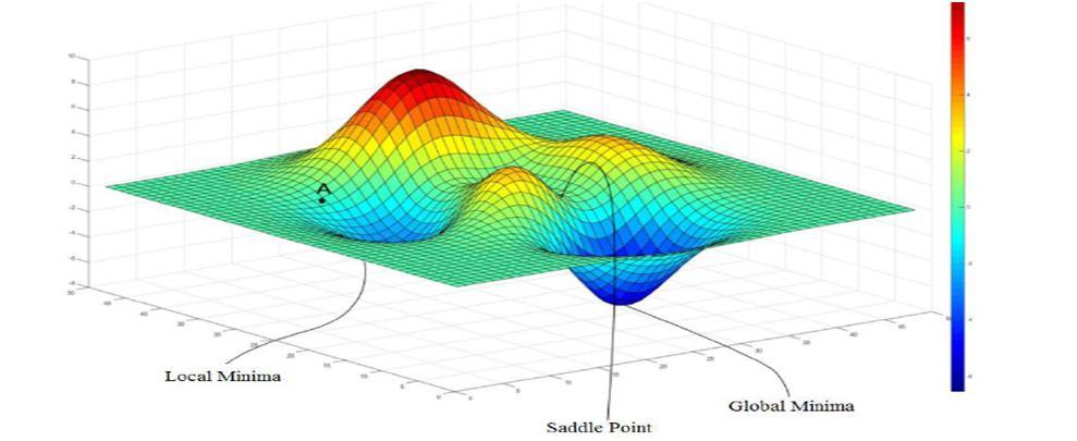
The cruciality's of optimization issues in DL are fairly complex, and a pictorial representation is in Fig.2 with recitation as in Fig (i) Making the algorithm starts run and converging to a realistic result. (ii) Making the algorithm to assemble presto and speed up confluence rate. (iii) Icing confluence with a dumpy valuation – like global minimum.

Fig. 2. Optimization: Issues and Challenges

B. Stochastic GD Optimization

Ironically, SGD nearly succeed the grade of amini -batch tagged at arbitrary. While training a network, we estimate the grade using a suitable loss function. At a replication ‘k’, the grade will be streamlined consequently. Hence, the computation for ‘m’ exemplifications input from the training set having y (i) as target, is: ĝ ←1/m ∇ θ ( ∑ L (f (x(i) ; θ, y(i) ) (1)

Technology (IJRASET

ISSN: 2321-9653; IC Value: 45.98; SJ Impact Factor: 7.538 Volume 10 Issue XII Dec 2022- Available at www.ijraset.com

Here ‘η’ (eta) is getting rate. Further, the literacy rate is of consummate significance as the consequence of an update at ‘kth’replication is directed by this. For case, if η = 0.01 (certifiably small to small), also putatively more number of replication updates will be needed for confluence. On the negative, if η = 0.5 or further, also in this case the recent updates shall be largely dependent on the recent case. ultimately, an egregious wise decision is to elect(choose) it arbitrary by trial this is one veritably important hyperactive- parameter tuning in DL systems. On the resemblant side of it, yet another way could be ‘choose one among several literacy rates’ which give lowest loss value.

C. Stocastic Gradient Descent With Momentum

From the antedating section and paragraphs, it’s egregious that SGD has a trouble to get towards global optima, and has a tendency to get stuck into original minima, as depicted in Fig. 3. also, lower values of grade or noisy bones

Fig.

3. A 3-D Representation with Local and Global Minima (Maxima)

Can produce another problem of evaporating grade issue! To overcome this problem, the system involving instigation (a principle espoused from drugs) is espoused to accelerate the process of literacy. The instigation system aims to resolve 2 veritably important issues

(i) friction in SGD

(ii) friction when working Hessian Matrix for poor exertion

The system takes the brevity of running moving average by incorporating former update in the recent change as if there's a instigation due to antedating updates. The instigation- grounded SGD will meet briskly with reducing oscillations. To achieve this, we use another hyperactive- parameter ‘ν’ known as haste. This hyperactive- parameter tells the speed and of course the direction by which its moves in the given parameter space. Generally, ‘ν’ is set as negative of grade value of exponential decaying normal. Moving further on, we'd bear yet one further hyperactive- parameter α (nascence) α ϵ (0, 1), known as instigation parameter and its donation is to find how presto the former grade exponentially decays. The new (streamlined) values are computes as:

From equation( 2) it's egregious that the haste vector ‘ ν ’ keeps on adding the grade values. also, for a bigger value of α( nascence) relative to ϵ, the grade affects the current direction more from former replication. The generally used values of α from0.5 to0.99. Despite being so intuitive and nice fashion, the limitation of this algorithm is fresh parameter addition and redundant computations involved.

ISSN: 2321-9653; IC Value: 45.98; SJ Impact Factor: 7.538 Volume 10 Issue XII Dec 2022- Available at www.ijraset.com

D. Various Optimizers IN DL

The presently available optimizers with their process frame are compactly described with their relative graces and limitations. Each bone has some tricks or the other and an sapience of those will an exemplary study progression.

1) ADAGRAD

The simplest of optimizing algorithms to begin with is AdaGrad, where the algorithm’s names itself suggest, the algorithm adapts, i.e., stoutly changes the literacy rate with model’s parameters Then, for parameters whose partial outgrowth are advanced (larger) for them drop their corresponding literacy rate mainly. Contrary to this suspicion, the algorithm takes equally to where derivations are lower. A natural question to ask is ‘why one needs different literacy rates’? So, to negotiate these characteristics, AdaGrad employs square value of the grade vector using a variable ‘r’ for grade accumulation, as stated in following equation (3) ĝ ← αv – ε 1/m ∇ θ ( ∑ L (f (x(i) ; θ, y(i) ) (3)

Using this equation (3) the forecourt of grade is collected and latterly the update of parameters is reckoned by a scaling factor ‘ δ √ r ‘, where δ is a veritably low value constant for numeric stability. The update applied as per the following equation (4) now: r ← r + g g

Then ⨀ driver implieselement-wise addition of vectors. As can be inferred from above equations, when ‘ r ’ is close to a ‘ nearzero ’ value, the term in the denominator shouldn't be estimated as ‘ NaN = Not A Number ’ and therefore the term δ helps to avoid this to be. Also, the term ‘ ϵ ‘ stands for global literacy rate.

2) RMSPROP

The modified interpretation of AdaGrad is RMSProp – Root Mean Square Proportional [16]. In order to palliate the problems of AdaGrad, then we recursively define a decaying normal of all once slants. By doing so, the flowing exponential shifting normal at each time step depends only on the normal of former and current slants. It performs better in thenon-convex setting as well with same characteristics features. Comparison wise, AdaGrad contracts the literacy rate according to the entire history of the squared grade whereas RMSProp exploits an exponentially decaying normal to discard history from the extreme history similar that it can meet snappily after finding a convex coliseum. The equation to apply is: (5)

then ρ is the decay rate. also parameter update is computed and applied as follows: Δθ = - ϵ / ( δ + √ r ) g θ ← θ + Δθ (6)

3) ADAM

Adam( Adaptive momentum) one majorly used optimization algorithms in DL and joins the heuristic of both the momentum and RMSProp and interestingly been designed for deep neural nets [17]. This algorithmic fashion has the squared grade point of AdaGrad and to scale the learning rate similar to RMSProp and point of momentum using moving average. The fine algorithm calculates individual learning rate for each parameter using a term called ‘first moment’ (analogous to velocity vector) and ‘alternate moment’ (analogous to acceleration vector). A many salient features are:

ISSN: 2321-9653; IC Value: 45.98; SJ Impact Factor: 7.538 Volume 10 Issue XII Dec 2022- Available at www.ijraset.com

Momentum term is in- built as an estimate of first- order moment In-built bias correction while estimating for first and alternate order moments eventually called as initialization at origin( start point)

Update moving exponential pars of grade ‘ mt ’ and square grade ‘ ut ’ with hyperactive- parameters ρ1 and ρ2( in original paper by the authors, they're denoted by β1 and β2) as these control. These moving averages are estimates of the mean (first moment) and non-central variance (second moment) of the gradient. Continuing the pipeline process at time "t", the various estimates are: mt ← ρ1 mt-1 + (1-ρ1) gt ut ← ρ2 ut-1 + (1- ρ2) g g (7)

The bias is then corrected at the first and second moments. Parameter updates are computed and applied using the corrected moment estimates:

mt ← mt-1 / (1-ρ t 1) ut ← ut-1/ (1- ρ2) g Δθ ← mt-1 / (1-ρ t 1) θt ← θt-1 + Δθ (8)

Typical values from [28] are ρ1 (β1) = 0.9 and ρ2 (β2) = 0.999 and δ = 10 -8. Adam works quite well in deep learning scenarios and is one of the most favored adaptive learning-method algorithms.

4) YOGI Optimizer

One of the problems of Adam is that it can fail to converge even in convex settings when the second moment estimate blows up. As a fix [xxx] proposed a refined update optimizer called “Yogi” whose analysis is shown with respect to other optimizers [18].

IV. EXPERIMENTAL ANALYSIS

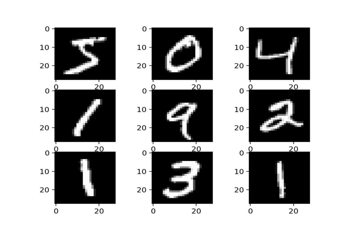
Simple MNIST ConvNet (CONVolutional neural NETwork) Handwritten Digit Classification (keras.io)

The MNIST dataset contains 60,000 small square 28×28 pixel gray scale images of handwritten single digits between 0 and 9 and to classify them into one of 10 classes representing integer values from 0 to 9.

Fig. 4. MNIST Hand-writing data

ISSN: 2321-9653; IC Value: 45.98; SJ Impact Factor: 7.538 Volume 10 Issue XII Dec 2022- Available at www.ijraset.com

The following tables provide insight on test results.

Table I Accuracy Results of Different Optimizer

O P T I M I Z E R

Epoc hs ADAM Ada Max Ada Grad

Ada Delta RMS Prop Yogi

1 0.98944 0.99391 0.99563 0.995722 0.99417 0.970204

2 0.990056 0.99481 0.995241 0.995593 0.99393 0.973518 3 0.990074 0.99444 0.995481 0.995759 0.99383 0.977556 4 0.990278 0.99496 0.995778 0.996241 0.99435 0.9815

5 0.990852 0.99493 0.995704 0.995685 0.99411 0.981926 6 0.990759 0.99493 0.995278 0.9955 0.99443 0.984481 7 0.991778 0.99509 0.995648 0.995574 0.99409 0.986241 8 0.991648 0.99511 0.99513 0.995519 0.99402 0.986204 9 0.991796 0.99533 0.996259 0.995463 0.99343 0.986833 10 0.992185 0.99561 0.995907 0.995815 0.99387 0.987426 11 0.992056 0.99557 0.995759 0.995926 0.9943 0.987648 12 0.992481 0.99528 0.995833 0.995315 0.99426 0.989611 13 0.99237 0.99509 0.995759 0.996148 0.99441 0.989704 14 0.993444 0.99539 0.995907 0.995926 0.99402 0.99037 15 0.992667 0.99552 0.995815 0.995741 0.99441 0.991056 16 NC NC NC NC NC NC

Table II Loss Calculations with increasing epochs

O P T I M I Z E R

ADAM AdaMax AdaGrad AdaDelta RMSProp Yogi 1 0.030769203 0.016840834 0.01342941 0.012349965 0.017442593 0.087317901 2 0.030660413 0.015531234 0.013289509 0.012383377 0.017121542 0.08579988 3 0.029737646 0.015701743 0.013125114 0.012387508 0.018014155 0.069638625 4 0.030144887 0.014686801 0.012907225 0.011606638 0.017465971 0.059331615 5 0.027279913 0.014767526 0.012580603 0.012971006 0.018059289 0.055165734 6 0.027382473 0.01386387 0.013189798 0.012643098 0.01771827 0.047942165 7 0.025238702 0.013591217 0.01279079 0.012046021 0.018092779 0.044593204 8 0.025885595 0.014543038 0.014221844 0.012886927 0.017295152 0.042187933 9 0.023921942 0.014223929 0.011225022 0.012647881 0.018683322 0.040300243 10 0.023671839 0.013068906 0.01282739 0.01188632 0.01872316 0.037228297 11 0.02272607 0.013204883 0.0121938 0.012444395 0.0178084 0.037166514 12 0.022571232 0.013990337 0.012817397 0.013405919 0.017346375 0.030976351 13 0.021767136 0.01409789 0.012786428 0.011781339 0.016602265 0.031661849 14 0.019936863 0.013202383 0.012017745 0.012444121 0.017100403 0.029365012 15 0.021123191 0.012833097 0.012669461 0.012824929 0.016711574 0.030113461 16 NC NC NC NC NC NC

Epoch s

ISSN: 2321-9653; IC Value: 45.98; SJ Impact Factor: 7.538 Volume 10 Issue XII Dec 2022- Available at www.ijraset.com

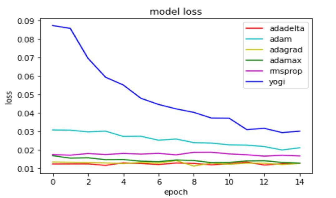
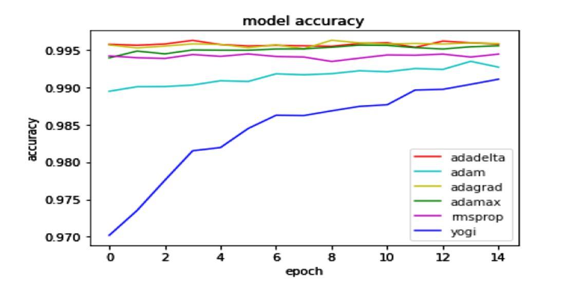
Figure 5 depicts their corresponding loss and accuracy plots.

Fig. 5. A comparative graph depicting various optimizers

V. OBSERVATION & DISCUSSION

ACCURACY ( Ref. Table I)

Adam After 14th Epoch, accuracy decreases and stays AdaMax a. After 16th Epoch, no change; b. Looks performing better than ADAM in this regard AdaGrad a. Started with higher accuracy and fluctuates more; b. not a good choice decision AdaDelta a. Started with higher accuracy and fluctuates more ; b. not a good choice decision

RMSProp Started with higher accuracy , but decreases Yogi a. Started with lower accuracy and increases ; b. seems to be good and better choice

LOSS ( Ref. Table II)

Adam Loss starts decreeing, however the fluctuating nature is observed

AdaMax Starts with low and decreasing nature noted AdaGrad Loss starts decreasing with increasing epochslooks performing pretty good on loss

AdaDelta Loss starts decreasing, however the fluctuating nature is observed

RMSProp Loss starts decreasing, however the fluctuating nature is observed

Yogi Loss starts decreasing with increasing epochs

ISSN: 2321-9653; IC Value: 45.98; SJ Impact Factor: 7.538 Volume 10 Issue XII Dec 2022- Available at www.ijraset.com

Several salient points emerge as they can be analyzed visually using different plots from the experimental analysis:

1) Each optimizer has its vividness and Adam and Yogi Optimizer’s loss gradually decreases with increasing accuracy with number of epochs. Others are either saturated or unable to generalize.

2) Except Adam and Yogi, the remaining one’s performances on this data set is monotonous and nothing indicative performance improvement is seen

3) Selecting a Particular Optimizer: Choose a well-understood optimizer with default learning rates and other parameters settings. Try changing these parameters in iterations (epochs) and see the loss (accuracy). Subsequently, shift towards other similarfeatured optimizer and observe the changes. This is indeed an exhaustive process!

VI. FUTURE SCOPE

We have provided intuitive way of reasoning based upon the experimental dataset. Moreover, various optimizers can be employed to test on different data sets and thus provide a valuable insight to select a particular one. Mostly, researchers’ guess rely on past experience or earlier cited proven examples. Furthermore, the entire ML and DL literature is slender with merits and demerits as compelling reasons. Also, getting an overview of their criticalities and understanding the reasons for choice makes a footing platform in ML [37,38,39]. Importantly, the optimizer and their intricacies area provide lot of scope for exploration and results could be agnostic in terms of accuracy of the model and eventually their performance.

REFERENCES

[1] Ian Goodfellow, Yoshua Bengio and Aaron Courville, Deep Learning MIT Press, USA 2016

[2] Bishop, C.M., Neural Network for Pattern Recognition, Clarendon Press, USA 1995

[3] François Chollet, Deep Learning with Python, Manning Pub., 1st Ed, NY, USA, 2018

[4] Ajeet K. Jain, Dr. PVRD Prasad Rao and Dr. K Venkatesh Sharma;”A Perspective Analysis of Regularization and Optimization Techniques in Machine Learning”,Computational Analysis and Understanding of Deep Learning or Medical Care: Principles, Methods and Applications". CUDLMC 2020 , WileyScrivener, April/May 2021

[5] John Paul Mueller and Luca Massaron, Deep Learning for Dummies, John Wiley, 019

[6] Josh Patterson and Adam Gibson, Deep Learning: APractitioner’s Approach, O’Reilly Pub. Indian Edition, 2017

[7] Ajeet K. Jain, Dr.PVRD Prasad Rao , Dr. K. Venkatesh Sharma, Deep Learning with Recursive Neural Network for Temporal Logic Implementation, International Journalof Advanced Trends in Computer Science and Engineering, Volume 9, No.4, July – August 2020, pp 6829-6833

[8] Srivasatava et al. http://jmlr.org/papers/volume15/srivastava14a.old/srivastava14a.pdf

[9] Dimitri P. Bertsekas, Convex Optimization Theory, Athena Scientific Pub., MIT Press, USA 2009

[10] Stephen Boyd and Lieven Vandenberghe, Convex Optimization, Cambridge University Press, USA 2004

[11] LeCun, Y., Boser, B., Denker, J. S., Henderson, D., Howard, R. E., Hubbard, W., and Jackel, L. D. (1989). Backpropagation applied to handwritten zip code recognition. Neural Computation, 1(4):541–551

[12] Hinton, G., Srivastava, N., Krizhevsky, A., Sutskever, I., and Salakhutdinov, R. Improving neural networks by preventing co-adaptation of feature detectors.arXiv:1207.0580, 2012

[13] Glorot, X. and Bengio, Y., Understanding the difficulty of training deep feed forward neural networks. In Proceedings of the International Conference on Artificial Intelligence and Statistics (AISTATS), pages 249–256. (2010)

[14] Glorot, X., Bordes, A., and Bengio, Y, Deep sparse rectifier neural networks. In Proceedings of the International Conference on Artificial Intelligence and Statistics (AISTATS), pages 315–323. 2011.

[15] Zeiler, M. and Fergus, R. , Stochastic pooling for regularization of deep convolutional neural networks. In Proceedings of the International Conference on Learning Representations ,ICLR, 2013Fabian Latorre, Paul Rolland and Volkan Cevher,Lipschitz Constant Estimation Of Neural Networks Via Sparse Polynomial Optimization, ICLR 2020

[16] D. Kingma and J. Ba, Adam: A method for stochastic optimization, arXiv:1412.6980, 2014

[17] Manzil Zaheer, et al., Adaptive Methods for Nonconvex Optimization, 32nd Conference on Neural Information Processing Systems (NeurIPS 2018), Montréal, Canada