Arima Model with Box-Cox Transformed Univariate Variable in BSE Sensex

ISSN: 2321 9653; IC Value: 45.98; SJ Impact Factor: 7.538

Volume 10 Issue XI Nov 2022 Available at www.ijraset.com

Arima Model with Box-Cox Transformed Univariate Variable in BSE Sensex

N Ramachandra1, M Bhupathi Naidu2, Sk Nafeez Umar3, K Murali4

1Research Scholar, Department of Statistics, 2Professor, DDE, S.V. University, 4Academic Consultant, Department of Statistics S.V. University

3Assistant Professor, Dpt. of Statistics and Computer Applications, S.V. Agricultural College

Abstract: Fluctuation of the stock market’s impact on investments of stocks. Sensex prediction plays an important role in the investment of markets. Predicting the stock market is difficult in market scenarios. The present study attempted to predict the stock market due to its complicated features and also compared different Auto Regressive Integrated Moving Average (ARIMA) models to get the appropriate stock forecasting model using various Box Cox transformations by using BSE Sensex past daily closing data. The ARIMA Model6 (0 1 0) showed accurate results in calculating the Mean Absolute Percentage Error (MAPE) and Bayesian Information Criterion (BIC) values, which indicates the potential of using the ARIMA model for accurate stock forecasting.

Keywords: ARIMA, MAPE, Box Cox transformation, BSE Sensex,

I. INTRODUCTION

Closing prices or returns on stock prices or closing values of the market as a whole is a kind of time series which in the series analysis is classified under “general random walk”. This is a non stationary time series which means its mean or other statistical properties change over time. The present study is the forecasting of the BSE Sensex index of stock and the daily BSE Sensex index data series This is daily data series of the BSE Sensex index The following is the description of the data set used in the research study. As per the review collected from various articles, many researchers have investigated volatility time series modeling of the different stock markets, mainly focusing on U.S and Indian stock markets. Some of the researchers have focused on the Indian stock market with ARIMA Model. The foremost drive of the study is to deepen the knowledge about stock market volatility in National Stock Exchange.

Rakesh Gupta (2012) aimed to forecast the volatility of stock markets belonging to the five founder members of the Association of South East Asian Nations, referred to as the ASEAN 5 by using Asymmetric PARCH (APARCH) models with two different distributions (Student t and GED). The result showed that APARCH models with t distribution usually perform better.

Praveen (2011) investigated BSE SENSEX, BSE 100, BSE 200, BSE 500, CNX NIFTY, CNX 100, CNX 200 and CNX 500 by employing ARCH/GARCH time series models to examine the volatility in the Indian financial market during 2000 14. The study concluded that extreme volatility during the crisis period has affected the volatility in the Indian financial market for a long duration. Philip Hans Franses & Dick Van Dijk (1996) Forecasting stock market volatility using (nonlinear) GARCH model, as per the finding of the study Q GARCH model is best when the estimation sample does not content extreme observations such as the 1987 stock market crash and the GJR model cannot be recommended for forecasting. In their estimation of volatility they used Within Sample Estimation and Out of Sample estimation and found that the forecasting performance of the GARCH type models appears sensitive to extreme within sample observations.

Srinivasan et al. (2010) attempted to forecast the volatility (conditional variance) of the SENSEX Index returns using daily data, covering a period from 1st January 1996 to 29th January 2010. The result showed that the symmetric GARCH model do perform better in forecasting conditional variance of the SENSEX Index return rather than the asymmetric GARCH models

Floros (2008) the researcher has investigated the volatility using daily data from two Middle East stock indices viz., the Egyptian CMA index and the Israeli tase 100 index, and has used various models, GARCH, EGARCH, TGARCH, Component GARCH (CGARCH), and Power GARCH (PGARCH).

The study found that the coefficient of the EGARCH model showed a negative and significant value for both indices, indicating the existence of the leverage effect. AGARCH model showed weak transitory leverage effects in the conditional variances and the study showed that increased risk would not necessarily lead to an increase in returns.

ISSN: 2321 9653; IC Value: 45.98; SJ Impact Factor: 7.538 Volume 10 Issue XI Nov 2022 Available at www.ijraset.com

II. MATERIAL AND METHODS

The Bombay Stock Exchange (BSE) data were considered for applying the time series models like ARIMA using various Box Cox transformations in the time series data. The present study is based on the daily closing market index for the Bombay Stock Exchange (BSE). Actively performing BSE Sensex (Aug 2008 Aug 2022) used for forecasting modes. In this study, Statistical software and R language were used for the forecasting model building.

III. DIAGNOSTIC CHECKING

A. Outliers Checking

An outlier is a value or an observation that is distant from another observation, differs point that differs significantly from other data points Grubbs's test is based on the assumption of normality to check whether the data follows normality or not. This is the foremost step for data should have any outliers.

That is, one should first verify that the data can be reasonably approximated by a normal distribution before applying the Grubbs test.

Grubbs's test detects one outlier at a time. Grubbs's test is defined for the hypothesis: H0: There are no outliers in the data set, Ha: There is exactly one outlier in the data set

The Grubbs test statistic is defined as

B. Data Normality

G= | | , , ,

Normality assumptions were used in the study of model building. In Jarque Bera normality test was used in this analysis for the normality of the data. The null hypothesis for this is data follows normal distribution; the alternative hypothesis is the data does not follow normality. The data uses thenormalized technique for time series indices of BSE indices data

The Jarque Bera test is a goodness of fit test of whether sample data have skewness and kurtosis matching a normal distribution The test is named after Carlos Jarque and Anil K. Bera. The test statistic is always non negative. If it is far from zero, it signals the data do not have a normal distribution.

JB= + ( 3) where n is the number of observations (or degrees of freedom in general); S is the sample skewness, k is the sample kurtosis

C. Box Cox Transformation

Generally, transformation plays a lead role in prediction of future values. A Box Cox transformation is a transformation of non normal dependent variables into a normal shape. Normality is an important assumption for many statistical techniques; if your data isn’t normal, applying a Box Cox means non normal to normalize the data. The following Box Cox transformation is an exponent, lamda (λ), which varies from 5 to 5, which all values λ are considered and the optimal value for the data selected

ISSN: 2321 9653; IC Value: 45.98; SJ Impact Factor: 7.538

Volume 10 Issue XI Nov 2022 Available at www.ijraset.com

Table1: Various Box Cox transformations

S No Model Transformation Model Lamda (λ) Transformed data (y)

1 Model 1 =1/y3 3 1/y3

2 Model 2 =1/y2 2 1/y2

3 Model 3 =1/y 1 1/y

4 Model 4 =1/sqrt(y) 0.5 1/sqrt(y)

5 Model 5 log(y) 0 log(y)

6 Model 6 =sqrt(y) 0.5 sqrt(y)

7 Model 7 y 1 y

8 Model 8 y 2 2 y 2

D. Model Selection and Forecasting

One of the concept in time series modeling is ARIMA, or Auto Regressive Integrated Moving Average. ARIMA is the combination of two models, the auto regressive and the moving average models. An auto regressive AR(p) component refers to the use of past values in the regression equation for the series Y. The auto regressive parameter p specifies the number of lags, or past values, to be used in the model. For example, AR(2) is represented as Yt=c+ϕ1yt 1+ϕ2yt 2 +…..+ ϕpyt p+et where φ1, φ2 are parameters for the model. The moving average nature of the model is represented by the “q” value, which is the number of lagged values of the error term. A moving average MA(q) component represents the error of the model as a combination of previous error terms et. The order q determines the number of terms to include in the model Yt=c+θ1e 1+θ2et 1+...+θqet q+et

Together, with the differencing variable d, which is used to remove the trend and convert a non stationary time series to a stationary one, these three parameters define the ARIMA model. Thus, ARIMA is specified by three order parameters: (p, d, q)

E. Stationarity Test

One of the imperative assumptions on time series is non stationary relationship. To make sure existence of stationary relationship, the following stationary test and Augmented Dickey Fuller test (ADF) were employed in the data

Where denotes the weekly index of the individual stock at time t, is the coefficient to be estimated, k is the number of lagged terms, t is the trend term, 2 is the estimated coefficient for the trend, 0 is the constant and is white noise

F. Mean Absolute Percentage Error (MAPE)

It measures this accuracy as a percentage, and can be calculated as the average absolute percent error for each time period minus actual values divided by actual values. A lowest percentage of MAPE is indicates good model for accuracy.

MAPE= ∑ Where n is the number of fitted points

G. Bayesian Information Criterion (BIC)

The BIC is general approach to model selection that favours more parsimonious models over more complex models (Schwarz, 1978; Raftery, 1995)

BIC = 2 * LL + log(N) * k

Where log() has the base e called the natural logarithm, LL is the log likelihood of the model, N is the number of examples in the training dataset, and k is the number of parameters in the model. The BIC value is minimized, the model with the lowest BIC is selected.

ISSN: 2321 9653; IC Value: 45.98; SJ Impact Factor: 7.538 Volume 10 Issue XI Nov 2022 Available at www.ijraset.com

IV. RESULTS AND DISCUSSIONS

Table1: Descriptive Statistics of BSE Sensex indices

BSE Index Descriptive Statistics

Mean 45603.37 Standard Error 297.00 Median 41543.45 Standard Deviation 9354.47 Kurtosis 1.39 Skewness 0.19 Range 35784.35 Minimum 25981.24 Maximum 61765.59 Count 992

From the above table, the mean value of BSE Sensex is 45603.37, the Standard Deviations of index is 9354.47. The skewness and 0.19 and 1.39 respectively, it means the distribution is longer than the right. The fig1 shows there is an increasing trend of BSE Sensex over the time period.

40000

30000

20000

10000

50000 511

70000 1 31 61 91 121 151 181 211

60000 571 601 631 661 691 721 751 781 811 841 871

241 271 301 331 361 391 421 451 481

541

Fig1: pattern of BSE Sensex data (2019 to 2022)

Table2: Diagnostic test of BSE Sensex

S No Test Test name Value p value

1 Outlier test Grubbs's test 3.4628 0.0753

2 Normality test Jarque Bera test 86.851 0.000

ISSN: 2321 9653; IC Value: 45.98; SJ Impact Factor: 7.538 Volume 10 Issue XI Nov 2022 Available at www.ijraset.com

Table3: Stationarity test of BSE Sensex

S No ADF test p value Difference Stationarity

1 2.0499 0.55772 Zero difference Non Stationarity 2 9.0314 0.0100** First difference Stationarity

Note ** Significant at 0.01 level

The Dickey Fuller test returns a p value of 0.01, resulting in the rejection of the null hypothesis and accepting the alternate hypothesis, it means the data is stationary. It is quite common in Sensex data. By taking the difference between BSE Sensex, we are essentially stationarizing the time series. Though not all stock returns are stationary, in many experiments regarding financial analysis, many assume it is.

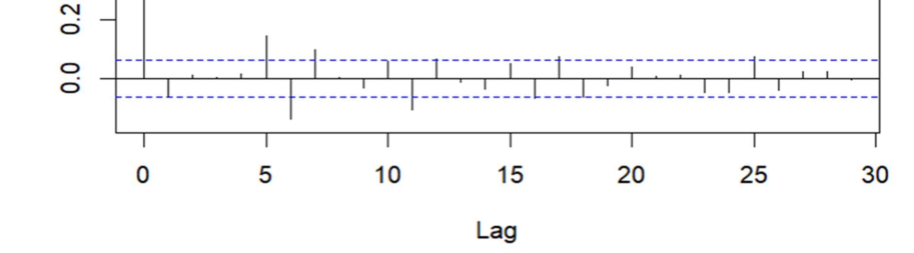
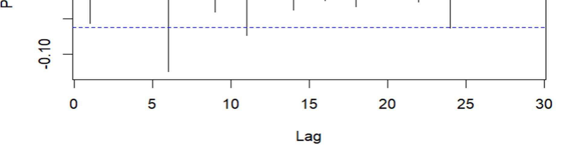
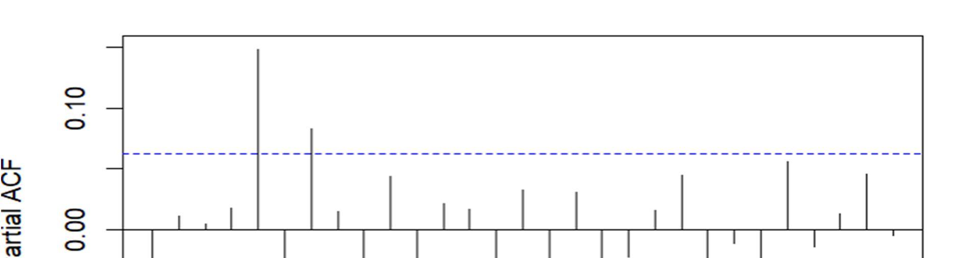
Fig1: ACF and PACF functions of BSE Sensex

ISSN: 2321 9653; IC Value: 45.98; SJ Impact Factor: 7.538 Volume 10 Issue XI Nov 2022 Available at www.ijraset.com

ACF stands for Auto Correlation Function. ACF gives us values of any auto correlation with its lagged values. In essence, it tells us how the present value in the series is related in terms with its past values. ACF will help us determine the number, or order, of moving average (MA) coefficients in our ARIMA model. PACF stands for Partial Auto Correlation Function. Instead of finding correlations of present with lags like ACF, it finds correlation of the residuals with the next lag value. If there is any hidden information in the residual which can be modelled by the next lag, we might get a good correlation and we will keep that next lag as a feature while modelling. PACF helps us identify the number of auto regression (AR) coefficients in our ARIMA model.

-4000 -2000 0 2000 0 200 400 600 800 1000

Residuals from ARIMA(0,1,0) -0.05 0.00 0.05 0.10 0 5 10 15 20 25 30 Lag

df$y

ACF 0 30 60 90 -4000 -2000 0 2000 residuals

The method used in this current study to develop ARIMA models for BSE Sensex explained in below table. The tool used for performance is R language five emerging stock indices daily data were used in this model. In this study the closing index is chosen to represent the index to be predicted. To determine the fitting best ARIMA model among the several combinations performed, the following criteria used in this modelling

1) Relatively small of Bayesian Information Criterion (BIC) 2) Relatively high of the R Square

3) Relatively low MAPE value

Table3: Model Performance of BSE Sensex

Model Transformation Model ARIMA Model R Square MAPE BIC value

Model1 =1/y3

ARIMA (0 0 1) 0.998 0.785 12.403

Model 2 =1/y2 ARIMA (0 1 0) 0.487 0.943 42.56

Model 3 =1/y ARIMA (0 0 1) 0.741 0.784 36.52

Model 4 =1/sqrt(y) ARIMA (0 0 0) 0.998 0.739 13.56

Model 5 log(y) ARIMA (1 0 0) 0.978 0.367 24.56

Model 6 =sqrt(y) ARIMA (0 1 0) 0.998 0.064 0.258

Model 7 y ARIMA (0 1 0) 0.958 0.071 14.52

Model 8 y 2 ARIMA (0 1 0) 0.956 1.720 35.65

The result of BSE Sensex, applied various type of Box Cox transformations and used best ARIMA models. From the Model6 the R square is 0.997, MAPE is 0.064 and BIC value is 0.258, which means higher R value, lower MAPE and BIC values for the above Model6. Conclude that Model6 which is the Box Cox transformation of SQRT(y) is the best appropriate model of BSE Sensex data.

ISSN: 2321 9653; IC Value: 45.98; SJ Impact Factor: 7.538 Volume 10 Issue XI Nov 2022 Available at www.ijraset.com

V. CONCLUSIONS

Difficult to the building of forecasting models mostly in time series data. Mainly in stock market data very oscillates over time. Forecasting with Auto ARIMA models provides a prediction based on historical data, in which data has been tested stationary and employed first order differences to remove white noise problems. In this study, Auto ARIMA estimated BIC, MAPE, and R Square which yielded a more accurate forecast over the time period and performance of the models. Thus, the study shows that the ARIMA model outperforms in forecasting BSE Sensex indices in terms of forecasting accuracy and in generating upcoming indexes.

REFERENCES

[1] Philip (1996). “Forecasting stock market volatility using non linear Garch models”, Journal of Forecasting, Vol. 15, pp. 229 235

[2] Floros Christos (2008). “Modelling volatility using GARCH models: Evidence from Egypt and Israel”, Middle Eastern Finance and Economics, No. 2, pp. 31 41

[3] Srinivasan P. and Ibrahim P. (2010). “Forecasting stock market volatility of Bse 30 index using Garch models”, pp. 47 60, available online at: https://journals.sagepub.com/doi/10.1177/097324701000600304

[4] Rakesh Gupta (2012). “Forecasting volatility of the ASEAN 5 stock markets: A nonlinear approach with non normal errors”, Griffith University

[5] Praveen Kulshreshtha (2011). “Volatility in the Indian financial market before, during and after the global financial crisis”, Journal of Accounting and Finance, Vol. 15, No. 3.

[6] Shaik Nafeez Umar Shaik and, Labeeb Mohammed Zeeshan (2009), Journal of Business and Economics, ISSN 2155 7950, USA November 2019, Volume 10, No. 11, pp. 1045 1056

[7] Sk Nafeez Umar.,etl (2017) Forecasting Of Cotton Area, Production, Productivity Using Arima Models In Andhra Pradesh, Bulletin of Environment, Pharmacology and Life Sciences Bull. Env. Pharmacol. Life Sci., Vol 6 Special issue [3] 2017: 138 141