Analysis of One-Dimensional Solute Transport of Arsenic in Aquifer via MT3DMS

ISSN: 2321 9653; IC Value: 45.98; SJ Impact Factor: 7.538

Volume 10 Issue X Oct 2022 Available at www.ijraset.com

Analysis of One-Dimensional Solute Transport of Arsenic in Aquifer via MT3DMS

Vidya Bhushan

1,

Asit Singh

2

1

2

M.tech Scholar,

Assistant Professor, CED, Institute of Engineering and Technology, Lucknow, India

Abstract: Analysis of one dimensional solute transport of Arsenic in Dudhi region of Sonebhadra district Uttar Pradesh is presented in this study. To understand and predict the behavior of solute transport within the ground water simulation of solute transport is necessary and helpful to develop remediation for this pollution. In this study the transport behavior of contaminant transport incorporating with non linear sorption (Freundlich) for different adsorption capacities (Freundlich adsorption coefficient) (Kf) and adsorption intensity (Freundlich exponent) (a) is numerically simulated using MT3DMS. MT3DMS is a well know simulator for simulation of solute transport problems. For the study multiple simulations were conducted with several values of Kf and a, to study the trend analysis of breakthrough curves. For the visualization of the output of simulation and to plot the BTC the observation output files were imported to M.S. EXCEL and proceeded to plot the BTCs for trend analysis.

Keywords: Arsenic, Adsorption, Freundlich isotherm, solute transport, MT3DMS.

I. INTRODUCTION

Contamination of ground water is a major emerging challenge for us. Since we rely on groundwater for source of water in major parts of world, it must be entertained well. Whenever any foreign material or contamination finds it path down to the groundwater and joins the groundwater and pollutes water inside the earth aquifers is termed as Ground water contamination. In India the responsible contaminant for ground water pollution is generally identified are salinity, fluoride, nitrate, arsenic and other heavy metals. Trace of high levels fluoride above the acceptable limits of 1.5 ppm occur in around 14 states of our India. It is also reported that around 65 % of Indian rural areas are exposed to fluoride risk. Trace of high level salinity is also reported from several states. High levels of arsenic has been also found in the Ganga basin belt of several districts of UP, Bihar and West Bengal To understand and predict the behaviors of solute transport within the ground water simulation of reactive contaminants is necessary and very helpful to develop remediation for the pollution. Simulation can also be useful to predict the concentration of contaminant in any particular time at any particular space. Simulation of solute transport is done by solving the ADE (Advective dispersive differential equation) governing the transport mechanism with the help of computer programs and codes to get the study results and findings. It reduces our effort and save time as compared to other methods of solving ADE. In this current study for one dimensional solute transport with equilibrium controlled sorption, MT3DMS is used for the simulation. A general procedure to the simulation of reactive solute transport with groundwater in porous media like soil is by assuming it to be driven by a linear sorption isotherm (Fetter, 1993).

A. Study Area

Figure1: Map of study area, Dudhi Sonbhadra

ISSN: 2321 9653; IC Value: 45.98; SJ Impact Factor: 7.538 Volume 10 Issue X Oct 2022 Available at www.ijraset.com

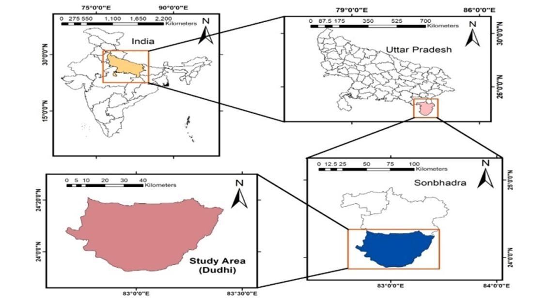
Geographically, the district is located between 23°52 and 24°55 N latitude and 82°30 to 83°33 E longitude. For the present work, two industrial clusters present in Dudhi region of SONBHADRA district, comprising of Obra (24°26303 24°48 4101 N and 82°5741.20 83°0248.90 E), Renukoot (24°11 17.20 24°1421.72 N and 83°00 22.50 83°0339.10 E) were selected. The study area is a hub for various industrial and commercial operations. The different industries present in the area are summarized as follows: Obra (Cluster A: Thermal Power Plant, Cement Factory, Sandstone limestone Mining), Renukoot (Cluster B: Chloro alkali Plant, Aluminum Smelting Plant and Hi tech Carbon Limited). The southern part of Uttar Pradesh’s Sonbhadra District and the north eastern part of Madhya Pradesh’s Singrauli District are popularly known as the ‘‘Energy capital of India’’. It is called so because of the presence of power grade coal reserves along with availability of water resources from Govind Ballabh Pant Sagar (G.B.P.S.) water reservoir (Rihand Dam). This provides an excellent location for other coal dependent industries like thermal power stations, aluminum smelting, cement industries, chloro alkali industry, hi tech carbon industry and other industrial and commercial operations adjacent to the coal mines (Khan et al. Khan. 2013). The surface and groundwater of Singrauli are severely contaminated due to direct pouring of fly ash slurry and leaching of toxic trace elements like As, Se, Hg, Cd and Pb from ash disposal pond of the power plant, making the water resources unfit for uses (Pandey et al. 2011).

II. METHODOLOGY

In this study the same problem is taken as illustrated in (Grove and Stollenwerk, 1984) considering the Freundlich & Langmuir isotherms. For our simulation MT3DMS was used and for creation of Input file all the steps were taken as directed in the MT3DMS user manual (Zheng et al., 2012).

A. Model parameters

The model parameters for the problem used for the simulation are same to that of (Grove and Stollenwerk, 1984) and they are illustrated below: Grid spacing (∆x) = 0.16 cm, Dispersivity (αL) = 1 cm, Groundwater seepage velocity (v) = 0.1 cm/s, Porosity (θ) = 0.37, Bulk density (ρb) =1.587 g/cm3, Freundlich equilibrium constant (Kf), Freundlich sorption exponent (a), Concentration of source fluid Co = 0.05 mg/l, Duration of source pulse (to) = 160 seconds For our study we will now see how the behavior of these breakthrough changes and what are the impacts on contaminant transport with the change in the Freundlich adsorption coefficient/ adsorption capacity (Kf) and Freundlich exponent constant/ adsorption intensity (a). All the other parameters are considered constant for proper analysis of adsorption phenomenon of soil for the heavy metals to get breakthrough curve. The Freundlich equilibrium constant and Freundlich sorption exponent has been calculated experimentally for the soil of particular study area. The soil sample collected from the Dudhi region of Sonbhadra district was used to calculate the adsorption capacity and adsorption intensity of Arsenic, the 20(gm) soil of all the soil sample was put in oven in a crucible dish at 105°C for 3 hours. Thereafter soil was taken out of oven and crushed finely and made to pass via 0.5mm sieve mesh, the 10(ml) standard solution of Arsenic was prepared which was later diluted 10 times for our experimental work. Then 10(gm) soil was mixed with 50(ml) of standard solution of Arsenic which was later put in centrifuge at 250 (rpm) for different time spans, after taking it out from centrifuge the sample was tested via Atomic absorption spectrometry to know the change in concentration of Arsenic in the standard solution. The data obtained was later put through analysis via Origin pro software to get the data below for the simulation of one dimensional solute transport.

TABLE 1: Binding Affinity And Capacity Parameters For Freundlich Isotherm Sorption

Metals R2 Kf N a = 1/n Ar 0.928 0.20 1.21 1.38 2.60 0.50 0.86

B. Solute transport modeling using MT3DS

For our study we have prepared two data sets

SET 1, Kf = varies between 0.1 to 1.0 and SP2 = a = 0.70

SET 2, Kf = varies between 0.1 to 1.0 and SP2 = a = 0.50 Above two data sets for two parameters were taken in consideration for the study and for each consideration the simulation was run separately and the outputs for each simulation for transport model were saved in separate folders to avoid the errors in the process of data visualization. Flow field is considered in steady state. Also, here Peclet number = 0.16, so that problem is not advection dominating.

ISSN: 2321 9653; IC Value: 45.98; SJ Impact Factor: 7.538

Volume 10 Issue X Oct 2022 Available at www.ijraset.com

Constant head B.C for flow model are taken at both by setting arbitrary hydraulic head to get desired Darcy flux. Since our study is based on Freundlich sorption isotherm which is a non linear isotherm empirical model/equation is described as: = Kf Ca Here,

Kf = Freundlich constant/Adsorption capacity, (L3M 1) a , a= Freundlich exponent/ adsorption intensity, dimensionless.

Retardation factor can be defined as: =1+ =1+

Since the flow field is steady state, only one stress period is required for the flow model. However, to accommodate the change in source concentration, two stress periods are used in the transport model.

The boundary conditions for the flow model are constant head at the two ends of the model domain with the values of hydraulic head set arbitrarily to establish the desired Darcy flux.

The boundary conditions for the transport model are specified total mass flux (third type) on the left and zero dispersive mass flux (second type) on the right.

The third type boundary condition is approximated by specifying the advective mass flux (where q is the rate of inflow or outflow across the boundary).

This is accomplished in the test problem by setting the concentration of the inflow at the constant head node on the left to 0.05 mg/L and zero for the first and second stress periods, respectively. The second type boundary condition is handled by setting it sufficiently far away from the source so that the plume does not reach it within the specified simulation time.

III. RESULT AND DISCUSSION

For this study all the breakthrough curves are plotted at a distance of 8 cm from the initial source point of the concentration for a concentration pulse input for to=160 seconds and the initial concentration Co=0.05 mg/l and the total time for simulation is taken as 1500 seconds.

Here C/Co shows the relative aqueous phase concentration at that point with respect to initial concentration and time unit of simulation is taken in seconds.

In this section we will do a trend analysis for the breakthrough curves for different 2 sets of Kf and a by varying the values of these parameters.

C/Co Time(sec)

0 500 1000 1500 2000

Figure 2: Breakthrough curve for a = 0.8 and Kf = 0.2

0.025

0.02

0.015

Kf = 0.3 and a = 0.8

A. Breakthrough Curves Obtained at a Distance 8 cm from source for a = 0.80 and Kf (SET 1). 0 0.005 0.01 0.015 0.02 0.025 0.03 0.035

Kf = 0.2 and a = 0.8 0

0.01

0.005

C/Co Time(sec)

0 500 1000 1500 2000

Figure 3: Breakthrough curve for a = 0.8 and Kf = 0.3

ISSN: 2321 9653; IC Value: 45.98; SJ Impact Factor: 7.538 Volume 10 Issue X Oct 2022 Available at www.ijraset.com

0 0.002 0.004 0.006 0.008 0.01 0.012 0.014 0.016 0.018 0.02 0 500 1000 1500 2000

C/Co Time(sec)

Kf = 0.4 and a = 0.8 0 0.002 0.004 0.006 0.008 0.01 0.012 0.014 0.016 0.018 0 500 1000 1500 2000

Figure 4: Breakthrough curve for a = 0.8 and Kf = 0.4

C/Co Time(sec)

C/Co Time(sec)

Figure 5: Breakthrough curve for a = 0.8 and Kf = 0.5

Figure 6: Breakthrough curve for a = 0.8 and Kf = 0.6

0.006 0.008 0.01

0.002 0.004

0.012 0 500 1000 1500 2000

C/Co Time(sec)

Figure 8: Breakthrough curve for a = 0.8 and Kf = 0.8

0.01

0.008

Kf = 0.5 and a = 0.8 0 0.002 0.004 0.006 0.008 0.01 0.012 0.014 0 500 1000 1500 2000

Kf = 0.6 and a = 0.8 0

0.006

0.004

Kf = 0.7 and a = 0.8 0

0.012 0 500 1000 1500 2000

C/Co Time(sec)

0.002

Figure 7: Breakthrough curve for a = 0.8 and Kf = 0.7

Kf = 0.8 and a = 0.8 0 0.001 0.002 0.003 0.004 0.005 0.006 0.007 0.008 0.009

Kf = 0.9 and a = 0.8

C/Co Time(sec)

0 500 1000 1500 2000

Figure 9: Breakthrough curve for a = 0.8 and Kf = 0.9

Science & Engineering Technology (IJRASET

ISSN: 2321 9653; IC Value: 45.98; SJ Impact Factor: 7.538 Volume 10 Issue X Oct 2022 Available at www.ijraset.com

0 0.001 0.002 0.003 0.004 0.005 0.006 0.007 0.008 0 500 1000 1500 2000

C/Co Time(sec)

Kf = 1.0 and a = 0.8 0 0.001 0.002 0.003 0.004 0.005 0.006 0.007 0 500 1000 1500 2000

C/C0 Time(sec)

Figure 10: Breakthrough curve for a=0.8 and Kf=1.0 Figure 11: Breakthrough curve for a=0.8 and Kf=1.1

Comparisons of breakthough curve when a = 0.8

0.03

0.025

0.02

0.015

0.01

C/Co Time(sec)

0.005

Kf=1.1 and a=0.8 0

0.035 0 200 400 600 800 1000 1200 1400 1600

Kf=0.2 Kf=0.3 Kf=0.4 Kf=0.5 Kf=0.6 Kf=0.7 Kf=0.8 Kf=0.9 Kf=1.0 Kf=1.10

Figure 12: Trend analysis via comparison between different values of Kf when a = 0.80

It can be seen as with increase in Kf value the peak of the breakthrough curve is being delayed and attenuation in the peak value is observed, the peak of breakthrough curve shows the maximum relative concentration value of the contaminant in dissolved aqueous phase. Attenuated and delayed peak for higher Kf value is observed than that of lower Kf value. At Kf value 0.8 the peak value starts to fade away and relatively lower peak values or flat graph is observed. At Kf = 0.1 we can see the peak value i.e maximum relative concentration (C/Co) in aqueous phase is above 3%of the initial released contaminant concentration and gradually decreasing with increased Kf also when Kf is 1.0 no peak is observed, curve is more like a flat line.

ISSN: 2321 9653; IC Value: 45.98; SJ Impact Factor: 7.538 Volume 10 Issue X Oct 2022 Available at www.ijraset.com

B. Breakthrough curves obtained at a distance 8 cm from source for a=0.60 and different values of (SET 2)

0.015

C/Co Time(sec)

0.01

0.005

0.02 0 500 1000 1500 2000

0

C/Co Time(sec)

0.01

0.008

0.006

Kf = 0.2 and a = 0.6 0

0.012 0 500 1000 1500 2000

0.004

0.002

C/Co Time(sec)

Figure 13: Breakthrough curve for a=0.6 and Kf=0.2 Figure 14: Breakthrough curve for a=0.6 and Kf=0.3

Figure 15: Breakthrough curve for a = 0.6 and Kf = 0.4

0.003

0.002

0.001

C/Co Time(sec)

0.004 0 500 1000 1500 2000

0.005

0.004

Kf = 0.3 and a = 0.6 0 0.001 0.002 0.003 0.004 0.005 0.006 0.007 0.008 0 500 1000 1500 2000

0.003

Kf = 0.4 and a = 0.6 0

C/Co Time(sec)

0.002

0.001

Kf = 0.5 and a = 0.6 0

0.006 0 500 1000 1500 2000

Figure 16: Breakthrough curve for a = 0.6 and Kf = 0 5

Kf=0.6 and a=0.6 0 0.0005 0.001 0.0015 0.002 0.0025 0.003 0.0035

Kf=0.7 and a=0.6

C/Co Time(sec)

0 500 1000 1500 2000

Figure 17: Breakthrough curve for a=0.6 and Kf=0.6 Figure 18: Breakthrough curve for a=0.6 and Kf=0.7

ISSN: 2321 9653; IC Value: 45.98; SJ Impact Factor: 7.538 Volume 10 Issue X Oct 2022 Available at www.ijraset.com

0.0025

0.002

0.0015

0.001

0.0005

C/Co Time (sec)

0

0 500 1000 1500 2000

Kf=0.8 and a=0.6 0 0.0002 0.0004 0.0006 0.0008 0.001 0.0012 0.0014 0.0016 0 500 1000 1500 2000

Figure 19: Breakthrough curve for a=0.6 and Kf=0.8

C/Co Time(sec)

Kf=0.9 and a=0.6 0 0.0001 0.0002 0.0003 0.0004 0.0005 0.0006 0.0007

C/Co Time(sec)

Figure 20: Breakthrough curve for a=0.6 and Kf=0 9

Kf=1.0 and a=0.6 0 0.00002 0.00004 0.00006 0.00008 0.0001 0.00012 0.00014 0.00016 0.00018

0 500 1000 1500 2000

Figure 21: Breakthrough curve for a=0.6 and Kf=1.0

Kf=1.10 and a=0.6

C/Co Time(sec)

0 500 1000 1500 2000

Figure 22: Breakthrough curve for a=0.6 and Kf=1.10

The trend and pattern obtained in both comparative analysis curve is very similar as it can be seen as with increase in Kf values the peak of breakthrough curve is delayed and attenuation in the peak value is observed, the peak of breakthrough curve shows the maximum relative concentration value of the contaminant in dissolved aqueous phase. Attenuated and delayed peak for higher Kf value is observed than that of lower Kf value. At Kf value 0.6 the peak value starts to fade away and relatively lower peak values or flat graph is observed. But at Kf= 0.1 we can see the peak value i.e maximum relative concentration (C/Co) in aqueous phase is nearly 1.8% of the initial released contaminant concentration and gradually decreasing with increased Kf also.

As seen with trends of breakthrough curve it has been observed that Kf make same impact to the breakthrough curve peak concentration and transport rate of contaminant but it more amount of contaminant is retarded when the a value is lower as compared to SET 1. It is observed that for same Kf values with a lower a value, the relative concertation of aqueous phase is higher than that of value with higher a. The solute migration rate and amount of solute migrated is lowered in each case as compared to previous set when a=0.80

ISSN: 2321 9653; IC Value: 45.98; SJ Impact Factor: 7.538 Volume 10 Issue X Oct 2022 Available at www.ijraset.com

Table 2: Comparison of Relative concentration values at a point 8 cm from the source of different Kf and a values

Maximum relative concentration (C/Co) at 8 cm distance from the source inaqueous dissolved phase within the simulation time.

Kf

When, a=0.6 When, a=0.8

0.2 0.0175 0.030

0.3 0.011 0.024

0.4 0.007 0.019

0.5 0.005 0.016

0.6 0.004 0.013

0.7 0.003 0.011

0.8 Negligible 0.010 0.9 Negligible 0.009 1.0 Negligible 0.0075 1.10 Negligible 0.0065

It can be seen clearly from the above table how the contaminant transport is being affected by these two parameters. C/Co= relative concentration in aqueous phase within the simulation time. Maximum relative concentration means the percentage of initial concentrationofinitial concentration input of dissolve aqueous phase at x = 0 and t=0.

IV. CONCLUSION

The solute transport of Arsenic contaminated ground water in the Dudhi region of Sonbhadra district has been analysed. This study indicates that with the increase in adsorption capacity (Kf) the concentration of contaminant dissolved in aqueous phase decrease since the more mass of contaminant is sorbed onto the solid phase. So the attenuation in peak relative concentration has been observed with increase in Kf values. This directly indicates that more the adsorption capacity of the soil slower the pollutant migration rate as the retention capacity of porous medium increases. The Freundlich exponent (a) or adsorption intensity has adverse effect on pollution migration, with high value of Freundlich exponent the concentration in aqueous phase increases as compared to the value of concentration in aqueous phase for a lower value of Freundlich exponent for same Adsorption capacity (Kf). Also, for same Kf at lower value of Freundlich exponent more retention of contaminant is observed also the peak is delayed but as the values of exponent increases the concentration in aqueous phase increases and the peak appears early since less retention of contaminant is offered by solid in this case. Hence the study gives the analysis of general behavior of soil with respect to Freundlich adsorption capacity and intensity, only using these parameters we could understand the change concentration of pollutants in aqueous phase.

V. ACKNOWLEDGEMENTS

The authors thank Asst. Prof. Asit Singh CED, IET Lucknow, their holistic support and Ecomen Laboratories Pvt. Ltd. Lucknow, to providing the essential facilities for conducting this research.

REFERENCES

[1] Fetter, C. W. (1993). Transformation, retardation, and attenuation of solutes. Contaminant Hydrogeology

[2] Khan, K., Lu, Y., Khan, H., Zakir, S., Khan, S., Khan, A. A., et al. (2013b). Health risks associated with heavy metals in the drinking water of Swat, northern Pakistan. Journal of Environmental Sciences, 25(10), 2003 2013.

[3] Pandey, V. C., Singh, J. S., Singh, R. P., Singh, N., & Yunus, M. (2011). Arsenic hazards in coal fly ash and its fate in Indian scenario. Resources, Conservation and Recycling, 55(9 10), 819 835.

[4] Zheng, C. et al. (2012) ‘MT3DMS: Model use, calibration, and validation’, Transactions of the ASABE, 55(4), pp. 1549 1559. doi: 10.13031/2013.42263

[5] Grove, D. B. and Stollenwerk, K. G. (1984) Computer model of one dimensional equilibrium controlled sorption processes, Water Resources Investigations Report.doi: 10.3133/wri844059.

[6] Agarwal, P. and Sharma, P. K. (2020) ‘Analysis of critical parameters of flow andsolute transport in porous media’, Water Science and Technology: Water Supply, 20(8), pp. 3449 3463. doi: 10.2166/ws.2020.

[7] Garg, S. and Singh, S. K. (2016) ‘Modeling of arsenic transport in groundwaterusing MODFLOW : A case study’, 6(4), pp. 56 81.

[8] Grove, D. B. (1985) ‘Modelling the rate controlled Sorption of HexavalentChromium’, 21(11), pp. 1703 1709.

ISSN: 2321 9653; IC Value: 45.98; SJ Impact Factor: 7.538 Volume 10 Issue X Oct 2022 Available at www.ijraset.com

[9] Grove, D. B. and Stollenwerk, K. G. (1984) Computer model of one dimensional equilibrium controlled sorption processes, Water Resources Investigations Report.doi: 10.3133/wri844059.

[10] Hulagabali, A. M., Solanki, C. H. and Dodagoudar, G. R. (2014) ‘Contaminant Transport Modeling through Saturated Porous Media Using Finite Difference andFinite Element Methods’, Mechanical and Civil Engineering, 2014, pp. 29 33.

[11] Igwe, J. C. and Abia, A. A. (2007) ‘Adsorption isotherm studies of Cd ( II ), Pb ( II )and Zn ( II ) ions bioremediation from aqueous solution using unmodified and EDTA modified maize cob’, 32(Ii), pp. 33 42.

[12] Kumar, M. D. and Shah, T. (2006) ‘Groundwater Pollution and Contamination inIndia : The Emerging Challenge’, India Water Portal, (January 2006), pp. 1 6.

[13] Liu, C., Ball, W. P. and Ellis, J. H. (1998) ‘An Analytical Solution to the One Dimensional Solute Advection Dispersion Equation in Multi Layer Porous Media’,pp. 25 43.

[14] Njuguna, S. M. et al. (2019) ‘Health risk assessment by consumption of vegetablesirrigated with reclaimed waste water: A case study in Thika (Kenya)’, Journal of Environmental Management, 231, pp. 576 581. doi: https://doi.org/10.1016/j.jenvman.2018.10.088.

[15] Rahman, M. M., Liedl, R. and Grathwohl, P. (2004) ‘Sorption kinetics during macropore transport of organic contaminants in soils : Laboratory experiments andanalytical modeling’, 40, pp. 1 11. doi: 10.1029/2002WR001946.

[16] Wu, J., Zhang, Y. and Zhou, H. (2020) ‘Groundwater chemistry and groundwater quality index incorporating health risk weighting in Dingbian County, Ordos basin of northwest China’, Geochemistry, 80(4, Supplement), p. 125607. doi: https://doi.org/10.1016/j.chemer.2020.125607.Zejia, L. I. U. et al. (2012) ‘Procedia Earth and Planetary Science The 2D FUPG Finite Element Model of Contaminant Transportation in Soil Considering NonlinearSorption’, 5, pp. 262 267. doi: 10.1016/j.proeps.2012.01.045.

[17] Majumdar, P. K., Ghosh, N. C., & Chakravorty, B. (2002), Analysis of arseniccontaminated groundwater domain in the Nadia district of West Bengal (India), Hydrological Sciences Journal, 47, pp S55 S66.

[18] Malik, V. S., Singh, R. K., & Singh, S. K. (2012a), Ground water modeling with processing modflow for Windows, (PMWIN) for the water balance study and suitable recharge site: case of Gurgaon district, Haryana, India. International Journal of Application or Innovation in Engineering & Management (IJAIEM), 1(1), pp 72 84.

[19] Njuguna, S. M. et al. (2019) ‘Health risk assessment by consumption of vegetablesirrigated with reclaimed waste water: A case study in Thika (Kenya)’, Journal of Environmental Management, 231, pp. 576 581. doi: https://doi.org/10.1016/j.jenvman.2018.10.088

[20] Rahman, M. M., Liedl, R. and Grathwohl, P. (2004) ‘Sorption kinetics during macropore transport of organic contaminants in soils : Laboratory experiments andanalytical modeling’, 40, pp. 1 11. doi: 10.1029/2002WR001946.