
10 VII July 2022 https://doi.org/10.22214/ijraset.2022.45989

A Study on Ordering Policy with Time-Varying Demand and Holding Cost for Deteriorating Items with Shortages
Abstract: The present paper focuses on time varying demand and holding cost, taking the same into consideration a finite horizon inventory problem for a deteriorating item has been developed for study. Deterioration rate is considered as a linearly time dependent. The demand rate varies with the time until the shortage occurs, but during the tenure of shortages it becomes static i.e. constant. Shortages are considered to be a partially backlogged in this study. In the study it is also considered that the backlogging rate is inversely proportionate to the length of the waiting time for next recovery. The main objective of the study is to minimize to the total cost of inventory with optimal order quantities of the products in the system. The graphs in the study show the convexity of the cost function. Finally, numerical results are discussed and presented in the section 5 of the study to analyze the degree of sensitivity of the optimal policies with respect to variations in the economic parameters of the model.
inventory models is having a finite planning horizon, time varying demand, and holding cost are worth Thenoting.rate of deterioration is considered to be linear in time. It is permissible to have a shortage that is partially backlogged. The main aim is to build an appropriate inventory models to non instantaneous deteriorating items over a finite planning horizon is the goal of this Shortagesresearch.and partial backlogs are allowed under the paradigm. The backlog rate varies depending on how long it takes for the next replenishment to arrive. The main goal is to calculate the best total cost and order quantity at the same time. We have demonstrated some numerical examples are presented. The sensitivity analysis is used to investigate the consequences of changing parameters.
The rest of our paper is laid out as follows: The literature on time varying demand, holding cost, deterioration rate, and backorder is reviewed in Section II. The assumptions and notation used throughout the paper are described in Section III. In Section IV, we established the main mathematical model. In Section V, focused on the solution to obtain total inventory cost and order quantity We have illustrated some numerical examples with sensitivity analysis and observations. Finally, we conclude in the section VI with the future work prospects.
International Journal for Research in Applied Science & Engineering Technology (IJRASET) ISSN: 2321 9653; IC Value: 45.98; SJ Impact Factor: 7.538 Volume 10 Issue VII July 2022 Available at www.ijraset.com 4398©IJRASET: All Rights are Reserved | SJ Impact Factor 7.538 | ISRA Journal Impact Factor 7.894 |
There are four forms of demand in the literature on inventory models namely, time dependent, stock dependent, constant demand, time and stock dependent and probabilistic demand. The majority of inventory models are predicated on the premise that an item's demand remains constant over the planning horizon. In reality, however the product demand cannot be fixed over time. It is dependent on inventory levels, selling prices and in some cases, time. Many scholars have been working on inventory models for decaying items in recent years. Deterioration of objects has become a typical occurrence in everyday life. Many things, including fruits, vegetables, pharmaceuticals, volatile liquids, blood banks, high tech products, and others, degrade with time due to evaporation, spoilage, obsolescence, and other factors. Inventory systems suffer from shortages as a result of deterioration, as well as a loss of goodwill or profit. As a result, degradation must be factored into inventory control models. Deteriorating products are seasonal things such as warm clothing, dairy products, green veggies, and so on. Shortages in the inventory system occur as a result of deterioration, affecting total inventory costs as well as total profit. As a result, another important component in the analysis of declining things inventory is the degrading rate, which indicates the nature of the items' Thedeterioration.studyofdeterministic
Keywords: Inventory model, deteriorating items, time dependent demand, shortages. I. INTRODUCTION
Dr. Mamta Sharma1 , Dr. Raveendra Babu A2 1, 2Department of Mathematics, Prestige Institute of Management and Research, Gwalior 474 020, M.P., INDIA

The first economic order quantity (EOQ) model was initiated by Harris (1915) for constant and known demand. Later on many researchers considered the variable demand such as, constant demand, time dependent, stock dependent, price dependent and probabilistic demand. Further, some researchers were worked on inventory with deteriorating items. Initially ‘A model for exponentially decaying inventory ‘was proposed by Ghare Nahmias (1975) suggested a perishable inventory model with constant demand for optimum ordering. Later Abad P (2001), Chung K.J. and Huwang Y.F. (2009), Shah N.H. AND Shukla (2009) Inventory models with time dependent demand rate were considered by Sivazlian and Stanfel (1976), Chung and Ting (1993) for replenishment of deteriorating items.
Due to shortages, the backlogging happens for which several researchers considered partial backlogging while some assumed fully backlogged inventory models. In practice, it is observed that at the time of the shortages either consumer wait for the arrival of next order (entirely backlogged) or they leave the system (entirely lacked). However, it is sensible to consider that, some consumers can wait to fulfill their demand during the stock out period (a case of full back order), whereas others don't wish to wait and fulfill their demand from another sources (a case of partial back order).
International Journal for Research in Applied Science & Engineering Technology (IJRASET) ISSN: 2321 9653; IC Value: 45.98; SJ Impact Factor: 7.538 Volume 10 Issue VII July 2022 Available at www.ijraset.com 4399©IJRASET: All Rights are Reserved | SJ Impact Factor 7.538 | ISRA Journal Impact Factor 7.894 | II. LITERATURE REVIEW
Several inventory models under the conditions of perishability and partial backordering for constant demand for optimal ordering policy were studied by Abad, P. (2001), Shah and Shukla (2009). Chung and Huang (2009), Hu and Liu (2010) developed optimal replenishment policy for deteriorating items with constant demand under condition of permissible delay in payment. An inventory model with time proportional demand for deteriorating items were developed by Dave & Patel (1981), Chung and Ting (1993), Chang and Dye (1999), Ouyang et al. (2005) with exponential declining demand and partial backlogging. Teng et al. (2007) studied the comparison between two pricing and lot sizing models with partial backlogging and deteriorating items. Alamri and Balkhi (2007) proposed a model for the effects of learning and forgetting on the optimal production lot size for deteriorating items with time varying demand. Some inventory models with ramp type demand rate, partial backlogging and weibull distributed deteriorating items are proposed by Jalan et al. (1996), Skouri et al. (2009), Mandal (2010), Hung (2011), Sana (2010). Kumar et al. (2012) proposed EOQ model with time dependent deterioration rate under fuzzy environment for ramp type demand and partial backlogging. In real life inventory model, the holding cost is also time dependant. Mishra (2014), Dutta and Kumar (2015), karmakar (2016), Chandra (2017) developed an inventory model for deteriorating items with time dependent demand and the time varying holding cost. Pervin et al. (2018) developed an EOQ model for time varying holding cost including stochastic deterioration. Hou (2006) developed an inventory model for deteriorating items with stock dependent consumption rate and shortages under inflation and time discounting Roy et al. (2011a, 2011b) proposed inventory models for imperfect items in a stock out situation with partial backlogging. Choudhary et al. (2015) developed inventory model for deteriorating items with stock dependent demand, time varying holding cost and shortages. Pervin et al. 2017) developed two echelon inventory model with stock dependent demand and variable holding cost for deteriorating items. Abad (1996) developed an EOQ model under conditions of perishability and partial backordering with price dependent demand. Dye (2007) developed an EOQ model with a varying rate of deterioration and exponential partial backlogging with price sensitive demand. Roy (2008) developed an inventory model for deteriorating items with price dependent demand and time varying holding cost. Sana (2010) proposed an EOQ model with time varying deterioration and partial backlogging. Shah et al. (2012) proposed an inventory model for optimisation and marketing policy for non instantaneous deteriorating items with generalised type deterioration and holding cost rates. Rastogi et al. (2017) developed an EOQ model with variable holding cost and partial backlogging under credit limit policy and cash discount. Sharma et al. (2018) developed an inventory model for deteriorating items with expiry date and time varying holding. Some products like fashionable and seasonal products are characterized by unpredictable demand.
Backlog shortages that occur will depend on the length of waiting time for the replenishment and is therefore the main factor for determining whether the backlogging will be accepted or not. For commodities with short life cycles like fashionable and high tech products, the rate of backorder is declining with the length of waiting time. The longer the waiting time is lower the backlogging rate, this results to a greater fraction of loss sales and hence a less profit as a consequence taking into the consideration of partial backlogging is necessary. Customers who have experienced stock out will be less likely to buy again from the suppliers, they might turn to another store to purchase the goods. The sales for the product might decline due to the introduction of more competitive product or the change in consumers’ preferences. The longer the waiting time, the lower the backlogging rate is. This leads to a larger fraction of lost sales and a less profit. As a result, taking the factor of partial backlogging into account is necessary.
Ordering cost per
Length
2) Inventory system contains single item 3) Considered the time horizon of the inventory system is finite.
4) Lead time to be zero. 5) Replenishment rate is infinite but size is finite.
7) For the time interval ≤ ≤ , the shortage is allowed and is partially backlogged with backordering rate: ( )= ( ) The backlogging rate is a positive constant. = , ( )= is the special case i.e. the fully backlogged case. In the projected model, we suppose δ < 1 for the approximation by Taylor’s Series.
Deterioration cost per cycle
Time
per
8) Holding cost is linear function of time: ( )=∝ +∝ t where ∝ ,∝ >0 are the scale parameters of holding cost.
Length
per
Inventory
T* Optimal value of T, where T is any variable ( ) Inventory level at time, 0≤ ≤ ( ) Inventory level at time, [0, ] ( ) Inventory level at time, [ , ] B. Assumptions 1) Demand rate, D(t)= + , 0≤ ≤ , ≤ ≤ , where , and >0 are arbitrary constants.
6) Rate of Deterioration is depending on time and there is no replacement of deteriorated units.
Deterioration
Purchase cost per
Maximum
International Journal for Research in Applied Science & Engineering Technology (IJRASET) ISSN: 2321 9653; IC Value: 45.98; SJ Impact Factor: 7.538 Volume 10 Issue VII July 2022 Available at www.ijraset.com 4400©IJRASET: All Rights are Reserved | SJ Impact Factor 7.538 | ISRA Journal Impact Factor 7.894 |
A. Notations Holding cost per
The demand of such items is low at the beginning of the season and increases as the season progresses, i.e., it changes with time, especially seasonal products like seasonable fruits, garments, shoes, etc. Most of these products have a lifespan of very short window in which to make the right calls on demand and procurement and achieve profits. There are three fundamental questions to answer such situations. How do sellers plan at firms selling such products for a season? How do they decide how much to order, when to schedule shipments and how much to mark down prices to reduce season ending inventory as much as possible? In this paper, we develop a deteriorating inventory model with the time dependent demand rate and deterioration rate. The unsatisfied demands will be partially backlogged. The backlogging rate is a variable and is inversely proportional to the length of the waiting time for next replenishment. So our aim is to minimize the total cost of inventory with optimal order quantity and optimal time of inventory exhausting. This paper is organized as follows: Section 2 describes the notations and assumptions, Section 3 presents the mathematical formulation of the problem, Section 4 provides a numerical example to illustrate the proposed inventory model, Section 5 discuss the sensitivity analysis, and finally Section 6 proposes the conclusions. unit unit time unit item unit item unit unit time of lost sales per unit rate of the cycle (Decision Variable) at which shortage starts, i.e., inventory exhausted time (decision variable), 0≤ ≤ of waiting time inventory level during a cycle of length T
Maximum amount of demand backlogged during a cycle of length T (= + ) order quantity during a cycle of length T holding cost per cycle
Cost
Shortage cost per cycle Lost sales cost per cycle T Average total cost per unit time per cycle
Shortage cost per
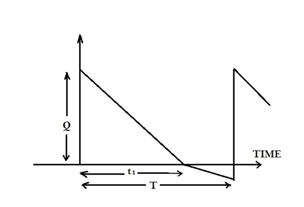
The changes in the inventory at any time t are governed by the differential equation during the periods [0, ] and [ , ] are respectively given by: ( ) + . ( )= ( + ),for0≤ ≤ (1) And ( ) = ( ),for ≤ ≤ (2) With boundary conditions ( )= ( )=0att= , ( )= =0 (3) The objective of this inventory problem is to determine the order quantity and length of ordering cycle so as to keep the total relevant costs as low as possible. That is, to determine Q* and T* so that the total cost is minimized. Now there are two cases: Case I: 0≤ ≤ In this case, the inventory level decreases due to the demand as well as deterioration, and the inventory level is governed by (1). Using the boundary conditions (3), the solution of (1) is given by ( )= ( )+ ( 3 +3 ) + [( )+ ( 4 +3 )] (4) Therefore, the maximum inventory level for each cycle = (0)= + + [ + ] (5) Case II: ≤ ≤ In this case, the inventorylevel depends due on demand. But a fraction of demand is backlogged. The inventorylevel is governed by (2). Using the boundary conditions (3), the solution of (2) is given by ( )= [log{1+ ( )} log{1+ ( )}], ≤ ≤ (6) Put t=T in (6), we obtain the maximum amount of demand backlogged per cycle as follows: = ( )= [log{1+ ( )}] (7) So, the order quantity per cycle is given by = + = + + + + log{1+ ( )} (8)
The objective of the model is to determine the optimal order quantity in order to keep the total relevant cost as low as possible. The inventory is replenished at time t = 0, when the inventory level is at its maximum W. Now, because of both the demand and deterioration of the item, the inventory level begins to decrease during the period [0, ], and finally becomes zero, when t= Further, during the period [ , ] the shortages are allowed, and the demand is assumed to be partially backlogged. The representation of inventory system at any time is shown in Figure 1.
Figure 1. Graphical presentation of inventory system
International Journal for Research in Applied Science & Engineering Technology (IJRASET) ISSN: 2321 9653; IC Value: 45.98; SJ Impact Factor: 7.538 Volume 10 Issue VII July 2022 Available at www.ijraset.com 4401©IJRASET: All Rights are Reserved | SJ Impact Factor 7.538 | ISRA Journal Impact Factor 7.894 | III. FORMULATION OF INVENTORY MODEL
International Journal for Research in Applied Science & Engineering Technology (IJRASET) ISSN: 2321 9653; IC Value: 45.98; SJ Impact Factor: 7.538 Volume 10 Issue VII July 2022 Available at www.ijraset.com 4402©IJRASET: All Rights are Reserved | SJ Impact Factor 7.538 | ISRA Journal Impact Factor 7.894 | For <1 , the Taylor’s series expansion yields the following second degree approximations: log{1+ ( )} ≈ ( ) ( ) (9) From equations (8) and (9), we get = + + + + [ ( ) ( ) ] = + + + + [( ) ( ) ] (10) Inventory holding cost per cycle is =∫ ( ) ( ) =∫ (∝ +∝ t) ( )+ ( 3 +3 ) + ( )+ ( 4 +3 ) = ( ( )+ ( + ))+ ( ( + )+ ) (11) Deterioration cost per cycle is = [ ∫ ( ) = + + + ∫ ( + ) = + (12) Shortage cost per cycle is given by = [ ∫ ( ) ] = [ ∫ [log{1+ ( )} log{1+ ( )}] = [( ) ( ) ] (13) Lost sale cost per cycle is given by = [∫ 1 ( ) ] = ( ) log{1+ ( )} = ( ) (14) So, the average total cost per unit time per cycle is TC= 1 [ + + + + ] ⇒ = 1 ( + ( 1 2( ) 1 3 ( ) )+ 1 2 ( ) + 1 2 ( 1 3 + 8 ) +( ( )+ ( + )) +( + ( + )) ) (15) So, the developed inventory model can be written as Minimize = 1 ( + ( 1 2( ) 1 3 ( ) )+ 1 2 ( ) + 1 2 ( 1 3 + 8 ) +( ( )+ ( + )) +( + ( + )) ) (16) Subject to ( )≥0, ≥0, ≥0 The problem is a single objective non linear optimization problem. The objective function TC is a function of and T. To find the optimality of and T, the partial derivative of TC with respect to and T are equated to zero and after solving these equations simultaneously we get the optimal values of and T. = ( ( )+ ( + ( ) + )+ ( + )+( ( )+ (2 + )) +( + ( + )) )=0 (17) = ( ) ( ( ) ) ( + ( ( )
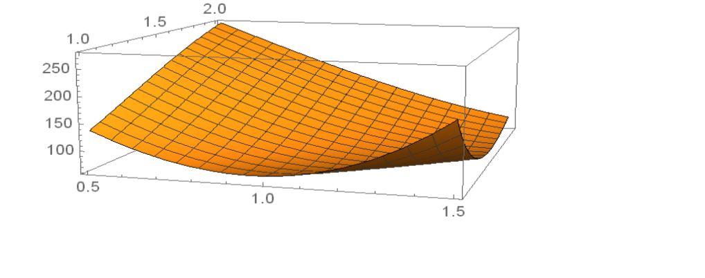
International Journal for Research in Applied Science & Engineering Technology (IJRASET) ISSN: 2321 9653; IC Value: 45.98; SJ Impact Factor: 7.538 Volume 10 Issue VII July 2022 Available at www.ijraset.com 4403©IJRASET: All Rights are Reserved | SJ Impact Factor 7.538 | ISRA Journal Impact Factor 7.894 | ( ) )+ ( ) + ( + )+( ( )+ ( + )) +( + ( + )) )= 0 (18) After solving equations (17) and (18) simultaneously, we obtain optimal values of and T and then substitute these values in equation (16) we get minimum average total cost per unit time of the inventory model. But the behavior of the cost function TC is highly non linear, so the convexity of cost function TC is shown graphically in the next section. Hence, the optimality of TC would be globally minimum. Numerical Problem: Let D(t)= 20+40 , 0≤ ≤ 25 ≤ ≤ , with =40, =20, , =25. Also ( )=0.5+0.011 where =0.5, = 0.011 >0. By using Mathematica software, we obtain the optimal solution of the problem ∗ =1.08772, ∗ =1.1412, shortage period = 1.1412 1.08772= 0.05348 unit, W* = 46.7644units and TC* = 66.3502 units. IV. CONVEXITY OF COST FUNCTION To show the convexity of cost function, we generate the graphs of total cost function C based on the parameter values taken in above examples. If we plot the total cost function with some values of and T, then we get the strictly convex graph of total cost function given by Figures 2, 3, 4, respectively. Figure 2: Convexity of cost function Figure 3: Total cost v/s at =11412 Figure 4: Total cost v/s at =09816 0.9 1.0 1.1 701.2 75 80 85 90 0.6 0.8 1.0 1.2 1.4 1.6 1.8 2.0 100 150 200 250 300
International Journal for Research in Applied Science & Engineering Technology (IJRASET) ISSN: 2321 9653; IC Value: 45.98; SJ Impact Factor: 7.538 Volume 10 Issue VII July 2022 Available at www.ijraset.com 4404©IJRASET: All Rights are Reserved | SJ Impact Factor 7.538 | ISRA Journal Impact Factor 7.894 | V. SENSITIVITY ANALYSIS Sensitivity analysis of various system parameters is required to observe whether the current solutions remain unchanged, then the current solutions become infeasible. Therefore, we analyze the effect of changes in various inventory system parameters: ∗, T*, W*, TC*. The sensitivity analysis is carried out by changing the value of each of the parameters by 20%, 10%, 20% and 10%, taking one parameter at time and keeping the remaining parameters unchanged. The results are displayed in Table 1. Parameter Value of parameter ∗ T* W* TC* 0.40 1.09762 1.1724 47.9016 63.7815 0.45 1.09264 1.1573 47.3443 650734 0.55 1.08285 1.1254 46.1923 67.6122 0.60 1.07804 1.1189 45.8468 68.8597 0.0088 1.1219 1.1783 49.0327 65.3827 0.0099 1.1056 1.1605 47.9426 65.8326 0.0121 1.0715 1.1237 45.707 66.8494 0.0132 1.0599 1.1112 44.9576 67.2264 3.2 1.08814 1.1415 46.7716 66.3148 3.6 1.08761 1.1410 46.7553 66.342 4.4 1.0871 1.1406 46.7255 66.3801 4.8 1.08657 1.1401 46.7135 66.4073 48 1.00542 1.0521 41.5007 57.7538 54 1.03244 1.0813 43.1976 62.599 66 1.11818 1.1743 48.7845 70.6117 72 1.16911 1.2298 52.249 74.0456 9.6 1.09295 1.1521 47.2332 65.979 10.8 1.08903 1.1451 46.9097 66.2068 13.2 1.08852 1.1398 46.7627 66.4233 14.4 1.08795 1.1371 46.6753 66.5292 12 1.09619 1.1575 47.4916 65.8117 13.8 1.08938 1.1456 46.9356 66.1922 16.5 1.08755 1.1381 46.6834 66.479 18 1.08291 1.1305 46.3175 66.7287 16 1.09478 1.1454 42.7627 65.1723 18 1.09245 1.1446 44.847 65.7273 22 1.07629 1.1305 48.2119 67.1691 24 1.07343 1.1291 50.249 67.7293 20 1.11179 1.1816 48.3566 65.1053 22.5 1.09395 1.1541 47.1741 65.9135 27.5 1.08405 1.1323 46.524 66.6702 30 1.07722 1.1209 46.0776 67.0548 32 1.15763 1.2088 45.8912 62.9931 36 1.11609 1.1681 46.0575 64.85 44 1.06388 1.1189 47.561 67.7112 48 1.03527 1.0911 47.8285 69.2199 0.0040 1.054 1.1045 44.5633 67.3853 0.0045 1.07691 1.1294 46.0515 66.6641 0.0055 1.08738 1.1409 46.7477 66.3712 0.0060 1.11151 1.1672 48.3509 65.703 0.64 1.10348 1.1581 47.8055 65.9073 0.72 1.09574 1.1498 47.2929 66.1216 0.88 1.08477 1.1381 46.5705 66.4336 0.96 1.07601 1.1287 45.9976 66.6943
as possible. The
, , , , , increases;
as
derivation and
(2 + 3 2 )+( (1 2 )+ 1 2 (4 + 2 5 )) +( 3 2 + ( + 2 )) ) = + (1 2 ( ))
of convexity of total coat TC ( , ) with respect to T and . For this objective we have to prove that ( , ) ( ,
=
5) When backlogging parameter increases, TC increases while W decreases and vice versa. Hence for minimum values of total cost TC, should be minimum that is back ordered rate should be as high above observations indicate that, in order to minimizing total cost, the policy should be to stock more to reduce the lost sale cost. Further, for avoiding high holding cost, low inventory level should be maintained strategically. Here have given proof ) ( , ) 0 Where 1 ( (1 2 ( ))+2 2( 2( 2 ( (2 6 )+ 30)) +( (6 + 40)) ) ( , ) ( 1+2
>
( , ) = 569.05195>0, ( , ) = 475.396>0 and ( , ) ( , ) ( , ) = 5039834>0
2) Order quantity W decreases as any one among , however it increases as increase.
( )= ( )
, ,
parameters
VII. APPENDIX
, , ,
= +
( )) 1 ( ( )+ ( + ( ) + )+ 1 2 ( + 2 ) +( ( 2 3 )+ 1 2 (2 + 2 15 )) +( 2 + (2 + 8 )) )
+ ( 1 2( ) 1 3 ( ) )+ 1
1
1 2 ( 2 3 +
1) Average total cost TC increases any of one among , , , however it decreases increases.
+
International Journal for Research in Applied Science & Engineering Technology (IJRASET) ISSN: 2321 9653; IC Value: 45.98; SJ Impact Factor: 7.538 Volume 10 Issue VII July 2022 Available at www.ijraset.com 4405©IJRASET: All Rights are Reserved | SJ Impact Factor 7.538 | ISRA Journal Impact Factor 7.894 | VI. OBSERVATIONS The following observations are made from sensitivity analysis:
Subsequently the above found cost function are enormously non linear therefore it is tough to develop the convexity mathematically. Therefore, some numerical values are taken the above example and graphs to develop the convexity (Figures By using numerical problem, we get which prove the convexity of total cost function.
in
VIII. CONCLUSIONS
8 +
, , , , increases;
we
3) Average total cost is more sensitive to the changes in ordering cost than other
2, 3 and 4).
4) Average total cost is relatively less sensitive to the changes in than other parameters
) + 1 2 ( 1 3 + 8 )+(
We proposed a deteriorating inventory model with time dependent demand rate and varying holding cost under partial backlogging along with time dependent deterioration rate. Shortages are allowed and partially backlogged. The classical optimisation technique is used to derive the optimal order quantity and optimal average total cost.
( )+ ( ( ) )) + 1
International Journal for Research in Applied Science & Engineering Technology (IJRASET) ISSN: 2321 9653; IC Value: 45.98; SJ Impact Factor: 7.538 Volume 10 Issue VII July 2022 Available at www.ijraset.com 4406©IJRASET: All Rights are Reserved | SJ Impact Factor 7.538 | ISRA Journal Impact Factor 7.894 | For the practical use of this model, we consider a numerical example with sensitivity analysis. Both the numerical example and sensitivity analysis are implemented the help of MATHEMATICA 8.0. The proposed model can assist the manufacturer and retailer in accurately determining the optimal order quantity, cycle time and total cost. Moreover, in market there are certain items where during the season period, the demand increases with time, and when the season is off, the demand sharply decreases and then becomes constant. Thereby, the proposed model can also be used in inventory control of seasonal items. This paper can be further extended by considering ramp type demand function. Further, the fuzzy or stochastic uncertainty in inventory parameters may be considered. REFERENCES
[18] Rangarajan, K.; Karthikeyan, K.: Analysis of an EOQ Inventory Model for Deteriorating Items with Different Demand Rates. Appl. Math. Sci. 9, 2255 2264 (2015)
[8] Goyal, S. and Giri, B. ‘Recent trends in modeling of deteriorating inventory’, European Journal of Operational Research, Vol. 134, No. 1, pp.1 16 (2001)
[6] Dye, C. ‘Determining optimal selling price and lot size with a varying rate of deterioration and exponential partial backlogging’, European Journal of Operational Research, Vol. 181, No. 2, pp.668 678 (2007)
[1] Abad, P. ‘Optimal pricing and lot sizing under conditions of perishability and partial backordering’, Management Science, Vol. 42, No. 8, pp.1093 1104 (1996)
[10] Jalan, A., Giri, R. and Chaudhary, K. ‘EOQ model for items with weibull distribution deterioration shortages and trended demand’, International Journal of System Science, Vol. 27, No. 9, pp.851 855 (1996)
[11] Kumar, R.S., De, S.K. and Goswami, A. ‘Fuzzy EOQ models with ramp type demand, partial backlogging and time dependent deterioration rate’, International Journal of Mathematics in Operational Research, Vol. 4, No. 5, pp.473 502 (2012)
[16] Palanivel, M.; Uthayakumar, R.: An EPQ model for deteriorating items with variable production cost, time dependent holding cost and partial backlogging under inflation. OPSEARCH 52, 1 17 (2015)
[19] Karmakar, B.: Inventory models with ramp type demand for deteriorating items with partial backlogging and time varing holding cost. Yugosl. J. Oper. Res. 24, 249 266 (2016) [20] Alfares, H.K.; Ghaithan, A.M.: Inventory and pricing model with price dependent demand, time varying holding cost, and quantity discounts. Comput. Ind. Eng. 94, 170 177 (2016) [21] Giri, B.C.; Bardhan, S.: Coordinating a two echelon supply chain with price and inventory level dependent demand, time dependent holding cost, and partial backlogging. Int. J. Math. Oper. Res. 8, 406 423 (2016) [22] Pervin, M.; Roy, S.K.; Weber, G.W.: A Two echelon inventory model with stock dependent demand and variable holding cost for deteriorating items. Numer. Algebra Control Optim. 7, 21 50 (2017) [23] Chandra, S.: An inventory model with ramp type demand, time varying holding cost and price discount on backorders. Uncertain Supply Chain Manag. 5, 51 58 (2017) [24] Rastogi, M.; Singh, S.; Kushwah, P.; Tayal, S.: An EOQ model with variable holding cost and partial backlogging under credit limit policy and cash discount. Uncertain Supply Chain Manag. 5, 27 42 (2017)
[9] Hung, K. ‘An inventory model with generalized type demand, deterioration and backorder rates’, European Journal of Operational Research, Vol. 208, No. 3, pp.239 242 (2011)
[15] Mishra, V.K.: Controllable deterioration rate for time dependent demand and time varying holding cost. Yugosl. J. Oper. Res. 24, 87 98 (2014)
[4] Chung, K.J. and Ting, P.S. ‘A heuristic for replenishment of deteriorating items with a linear trend in demand’, Journal of Operational Research Society, Vol. 44, No. 12, pp.1235 1241(1993)
[2] Abad, P. ‘Optimal price and order size for a reseller under partial backlogging’, Computers and Operation Research, Vol. 28, No. 1, pp.53 65 (2001)
[13] Ouyang, L.Y., Wu, K.H. and Cheng, M.C. ‘An inventory model for deteriorating items with exponential declining demand and partial backlogging’, Yugoslav Journal of Operations Research, Vol. 15, No. 2, pp.277 288 (2005)
[25] Pervin, M.; Roy, S.K.; Weber, G. W.: Analysis of inventory control model with shortage under time dependent demand and time varying holding cost including stochastic deterioration. Ann. Oper. Res. 260, 437 460 (2018a)
[5] Dave, U. and Patel, L. ‘(T, si) policy inventory model for deteriorating items with time proportional demand’, Journal of Operational Research Society, 32, 2, 137 142 (1981)
[27] Sen, N.; Saha, S.: An inventory model for deteriorating items with time dependent holding cost and shortages under permissible delay in payment. Int. J. Procure. Manag. 11, 518 531 (2018)
[14] Mandal, B. ‘An EOQ inventory model for Weibull distributed deteriorating items under ramp type demand and shortages’, OPSEARCH, Vol. 47, No. 2, pp.158 165 (2010)
[7] Ghare, P.M. ‘A model for exponentially decaying inventory’, The Journal of Industrial Engineering, Vol. 5, No. 14, pp.238 243 (1963)
[12] Roy, A. ‘An inventory model for deteriorating items with price dependent demand and time varying holding cost’, Advanced Modelling and Optimization, Vol. 10, No. 1, pp.25 37 (2008)
[17] Choudhury, K.D.; Karmakar, B.; Das, M.; Datta, T.K.: An inventory model for deteriorating items with stock dependent demand, time varying holding cost and shortages. OPSEARCH 52, 55 74 (2015)
[26] Pervin, M.; Roy, S.K.; Weber, G.W.: An integrated inventory model with variable holding cost under two levels of trade credit policy. Numer. Algebra Control Optim. 8, 169 191 (2018b)
[3] Chang, H. and Dye, C. ‘An EOQ model for deteriorating items with time varying demand and partial backlogging’, Journal of the Operational Research Society, 50, 11, 1176 1182 (1999)
International Journal for Research in Applied Science & Engineering Technology (IJRASET) ISSN: 2321 9653; IC Value: 45.98; SJ Impact Factor: 7.538 Volume 10 Issue VII July 2022 Available at www.ijraset.com 4407©IJRASET: All Rights are Reserved | SJ Impact Factor 7.538 | ISRA Journal Impact Factor 7.894 |
[28] Sharma, S.; Singh, S.; Singh, S.R.: An inventory model for deteriorating items with expiry date and time varying holding cost. Int. J. Procure. Manag. 11, 650 666 (2018)
[29] Geetha, K.V.; Naidu S.R.; Economic ordering policy for deteriorating items with inflation induced time dependent demand under infinite time horizon. Int. Journal of Operational Research. 39(1):69 94 (2020)
[30] Khatri, P.D.; Gothi, U.B.; An EPQ Model for Non Instantaneous Weibully Decaying Items with Ramp Type Demand and Partially Backlogged Shortages. Int. J. of Math. Trends and Tech. (IJMTT) (66)3 (2020)
[31] Adak, S.; Mahapatra, G.S.; Effect of reliability on varying demand and holding cost on inventory system incorporating probabilistic deterioration. American Institute of Mathematical Sciences 18(1): 173 193 (2022)