A Fixed-Point Approach to Mathematical Models in Epidemiology
Amelia BucurFaculty of Sciences, Department of Mathematics and Informatics, Lucian Blaga University of Sibiu, Sibiu, Romania
Email Id: amelia.bucur@ulbsibiu.ro
DOI:10.5281/zenodo.7375613
Abstract
Pandemics have always posed a great problem in the history of the world, leading to fatal dangers, which is why mathematicians have been challenged to bring their contribution to the management of pandemics, by applying their theoretical paradigms in describing, studying and forecasting their evolution. Compartmental models, i.e. exponential systems, have been remarkable for studying the spread of epidemics. This paper has three objectives: to purpose a generalization of the SEIRV (SusceptibleExposed Infected Recovered Vaccinated) model for studying the spread of an epidemics and simulation; to present conditions of existence for a solution to the purposed generalized SEIRV model; and to calculate the reproduction number in certain state conditions of the analyzed dynamic system. The conclusions are that, generally, mathematical models with many parameters can be used to forecast epidemics with better accuracy and, also, the elements from the theory of fixed points for multivalued operators can be used for the analysis of epidemics.
Keywords: mathematical modeling; epidemiological dynamics; fixed points 2010 Mathematics Subject Classification: 03C95, 47H10
Introduction
In many studies of pure and applied mathematics, the fixed point theory has significant applications It was and is an important tool in the research of linear or non linear problems from real life, and, have been applied in many fields such as: economics, computer science, algorithms, biology, genetics, engineering, chemistry, physics, optimizations, game theory, astronomy, geometry, mechanics, linear algebra, number theory, numerical analysis, complex analysis, transformational geometry, theory of chaos, etc. (Nalawade & Dolhare, 2016, p. 131)
The theory of fixed points includes conditions in which the single functions or multivalued functions admit fixed points. Fixed points was defined as roots of the equality, respectively inclusions in the following type: x = f(x), respectively x ∈F(x). Initially, the fixed point theory emerged in a work of Joseph Liouville, a remarkable French mathematician and engineer. Joseph Liouville published in the year 1837 an article for demonstrating existence of solutions of differential equations (Liouville, 1837, pp. 22 26) In year 1890, another mathematician, Charles Émile Picard from France, improved the sequence of successive approximations (Picard, 1890, pp. 156 158).
This method was used in a first fixed point theorem in complete normed spaces (Stefan Banach, 1922). In fact, the faimous polish mathematicians, Stefan Banach, was gives the first metric fixed point theorem which is known as the Banach Contraction Principle. This principle gives for functions f contractions, the existence and also the uniqueness of a fixed point. Also, the Banach Contraction Principle gives the method of the successive approximations, i.e. method to construct o sequence which converge to the fixed point for a contraction. The concept of contraction mapping was defined as:
Definition. Let (X, d) be a complete metric space. Then, a map is called a contraction mapping on X, if there exists a real constant ∈ such that the folowing inequality take place: for all ∈ (Ciesielski, 2007, p. 6).
© 2022, IJASRW, All right reserve https://www.ijasrw.com
International Journal of Advance Study and Research Work (2581-5997)/ Volume 5/Issue 11/November 2022
Also, some authors also applied elements of fixed point theory to analyze the solutions of mathematical models in epidemiology (i.e. Leggett, 1980, pp. 91 97; Lucas, 2013, pp. 135 149; Narsingani, Prajapati & Bhathawala, 2017, pp. 13 19; Tomar & Joshi (editors), 2021)
The theory may also be used to find existence conditions for the solutions of a mathematical model that predicts the spread of epidemics, as presented in this paper. Mathematical models of infectious disease dynamics utilizing ordinary differential equations have a long history of more than 200 years. In mathematical modeling for epidemiology, the following results are some from the remarkable results: the smallpox model created by Daniel Bernoulli (Bernoulli, 1766, pp. 1 45); the epidemic model realised by Roland Ross (Ross, 1911, pp.1 669); the SI (susceptible S; infected I) and SIS model (susceptible S; infected I; susceptible S) (Franke & Yakubu, 2006, pp. 1564 1585); the general epidemic model created by William Ogilvy Kermack and Anderson Gray McKendrick (the SIR (susceptible S; infected I; recovered R) model) (Kermack, McKendrick & Walker, 1927, pp. 702 716); the SEIR model; the MESIR (passive immune newborns M ; susceptible S ; exposed E ; infective I ; resistant (or immune) R) model (Hethcote, 2000, p. 618); the SEIRS model (an epidemic model with the saturation incidence) (Ross, 1911; Zhang & Teng, 2008, p. 65); the SEIRD (susceptible (S), exposed (E), infected (I), recovered (R), or dead (D)) and others. The results from the epidemic modeling are mathematical tools that contribute to analyze how diseases spread, and to forecast the state of an outbreak or to get and improve the strategies to decrease an epidemic (Braurer, 2017, pp .113 114; Hethcote, 2000, p. 599)
The mathematical models are very general and abstract, and are applicable not only to human diseases, but also to animal diseases (Kirkeby, Brookes, Ward, Dürr & Halasa, 2021, pp.2 10), plant diseases (van der Plank, 1963, pp.1 349), viral marketing and the spread of a computer virus (Rodrigues, 2016, 95 96).
Pandemics have posed extraordinary threats that have led to fatal dangers, in all of the human history. Thus, mathematicians have been challenged to bring their own contribution to managing pandemics, by applying their theoretical paradigms in order to describe, study, and forecast their evolution.
The type of the epidemic models can be: deterministic or stochastic. In all deterministic model the variables are uniquely determined by the initial state and the state of the parameters of the model. Specific to stochastic models is that all the variables are introduced by probability distributions. The models that we will consider in this paper will be deterministic models (Braurer, 2017, pp. 115 116; Hethcote, 2000, pp. 642 645)
Also, mathematical models that have been used in epidemiology are dynamic and statistic models. Every dynamic model accounts for time dependent changes in the state of the system. These models typically employ ordinary differential equations or systems of difference equations. A static model calculates system quantities assuming are time invariant. The models that we will consider in this paper are dynamic models (Braurer, 2017, pp .114 119; Hethcote, 2000, pp. 602 603)
On the other hand, the epidemic models are continuous or discrete models. In the continuous models time is from an interval of the set of real numbers, and in the case of the discrete models time in from a discrete subset of the set of the real numbers In the specialty literature, was used linear and nonlinear models. A model is defined as nonlinear if it include a nonlinear dependence on the variables. A model is a linear model, if it contains just linear dependences between the variables. The models from this paper are be nonlinear. On the other hand, mathematical models in epidemiology are compartmental models (Braurer, 2017, pp. 117 118; Hethcote, 2000, pp. 642 645)
For these models, in the specialty literature, exists the Akaike information criterion. It is a criterion for model selection that compares multiple competing models, taking into account both the SSE (the least squares error) and the number of parameters being fitted. The Akaike information criterion is a tool for measure of the relative goodness of fit of a mathematical model for a problem from real life, and was defined and was calculated as [ ( )] , where N is the volume of the data set, SSE is the least squares error, and k is the number of parameters fitted plus one The AIC has its foundations in the field of the information theory. Given a set of mathematical models, calculated the AIC for each model. A conclusion will be that the one with the smallest AIC is the best model. Obviously, a smaller SSE implies a smaller AIC, and, in this case, the model fits the dates the best. Also, a smaller k, implies that AIC is smaller for a volume smaller of the parameters (Martcheva, 2015, pp.135 136). Compartmental mathematical models in epidemiology, i.e. SI, SIS, SIR, MESIR, SEIRS, SEIRD or other models, was simulated in programs such as Mathematica (Srivastava, Area, Nieto, 2021, 3276 3284), GLEAMviz (Bucur, 2021, pp. 21 22), Maple (Bucur, 2021, pp.21 24), MATLAB (Area, Fernández, Nieto & Tojo, 2022, pp. 7459 7463), EPIDEMIC (Pavlack, Grave, Dantas, Basilio & de La Roca, et al., 2021, pp.2 5), C++ (Bouchnita, Chekroun, Jebrane, 2021, pp.7 10), Python (Abreu, Cantin & Silva, 2021, p. 7985 7986; Bouchnita, Chekroun & Jebrane, 2021, pp.6 10), SageMath (Abreu, Cantin & Silva, 2021, p. 7983), etc. Such models was applied in past pandemics, such as SARS (Severe acute respiratory syndrome), Swine flu, MERS (Middle East respiratory syndrome), Ebola and in present time, in study of the new epidemics such as COVID 19, MPXV (monkeypox), Tomato flu, etc. (i.e. Braurer, 2017, p .114; Calafiore, Novara & Possieri, 2020, pp. 366 369; Peter, Kumar, Kumari, Oguntolu, Oshinubi & Musa, 2022, pp. 3431 3433)
© 2022, IJASRW, All right reserve https://www.ijasrw.com
This work is licensed under a Creative Commons Attribution NonCommercial ShareAlike 4.0 International License
International Journal of Advance Study and Research Work (2581-5997)/ Volume 5/Issue 11/November 2022
Special attention is given to the studies stochastic epidemic mathematical models that substantiate computational epidemiology, physics, network science, etc. Along with these research directions, continuous development and the usage of increasingly better software may lead to important progress in other important issues raised by mathematical epidemiology. In present times, the scientific community of mathematicians and programmers are facing some key challenges (COVID 19 outbreaks, monkeypox outbreaks, tomato flu outbreaks) in terms of integrating the available data in mathematical models, meaning identifying the parameters of the models using the clinical and epidemiological data, which are sometimes incomplete. In order to solve this issue, researchers have suggested predictions or optimization methods (Calafiore, Novara & Possieri, 2020, pp. 362 369). The inclusion of behavioral factors in formulating mathematical models would also be an innovative aspect. In this regard, researchers have used game theory in order to showcase the use of self protective behaviors and in order to present people’s decision of getting or not getting vaccinated (Bauch & Earn, 2004, pp.13391 13394)
An important model that was validated by its practical application throughout the years is the SIR system. The SIR mathematical model is a dynamic one and it was created by Kermack and McKendrick in a paper published in the year 1927. In the specialty literature it was called as the classic epidemic model. The authors created a dynamic model with three compartments. The compartments was denoted by S (compartment of people susceptible to the infection), I (compartment of infected people), and R (compartment of recovered people). In these compartments take place the transfers: from S to I, from I to R. For construct the SIR system, was used the notations: S, I, and R are differentiable functions on the interval [0, ∞), S = S(t)= the number of people susceptible to the infection to each moment of time t, I = I(t)= the number of infected people to each moment of time t, R = R(t)= the number of people that have recovered from the illness to each moment of time t, where t represents a moment of time; β represents the rate of transmission. It is a parameter that controls the transfer between S and I. It represents the average number of contacts needed per time unit (per day) to infect a person; its relation to the number of contagious days depends firstly on applying social distancing measures, meaning if the person kept their distance from other people, from the moment they contracted the virus until they were diagnosed and placed into isolation; γ (or notation µ in some papers) notes the transfer rate between I and R. It was called the recovery rate. The invers of γ, 1/γ, shows the length of the time interval in which a person becomes infected. For example, for initial COVID 19 variants, from years 2019 2021, it was of 14 days. For the variants from years 2021 2022, specialists consider it to be of 5 days. The number of individuals, N, was considered by the authors of the SIR model to be constant. At any time t, by assuming that N (the statistical population volume) is a constant number, and S(t) + I(t) + R(t) = N William Ogilvy Kermack and Anderson Gray McKendrick (Kermack, McKendrick & Walker, 1927, pp. 700 721), using these notations and obtained an very important mathematical model, the SIR system: { (1)
which contain a non linear system of first order differential equations
In the first equation, the authors have highlighted mathematically that the variation in the number of susceptible people is directly proportional to the number of susceptible people at the moment of time t and, evidently, inversely proportional to the number of individuals at the moment of time t, which is, in fact, considered to be constant .
In the second equation, from (1) was shown mathematically that the variation in the number of infected people is directly proportional to the number of infected or susceptible individuals at the moment of time t and, evidently, inversely proportional to the number of individuals at the moment of time t, which is, in fact, considered to be constant . The third relation from the system of differential equations (1) shows that the variation in the number of recovered individuals is directly proportional to the number of infected people.
Initial conditions are
The initial moment of time is denoted by t = 0 and represented the moment from which is considered that the disease has started to spread, or the moment from which the analysis of the spread of an infectious disease has started. Initial conditions show the number of individuals susceptible to the infection at the moment of time ( ), the number of infected people at the initial moment of time ( ), and the number of recovered individuals at the initial moment of time ( ).
It is important to note that this model is applicable only to epidemics for which there are no vaccines available.
© 2022, IJASRW, All right reserve https://www.ijasrw.com
This work is licensed under a Creative Commons Attribution NonCommercial ShareAlike 4.0 International License
International Journal of Advance Study and Research Work (2581-5997)/ Volume 5/Issue 11/November 2022
For compartmental models in epidemiology, as well as for the SIR model, researchers have calculated reproduction numbers or bifurcation parameters. In report to 1 or another number, we can see the state of the dynamic system, meaning if the epidemic is spreading or ending (Hethcote, 2000, pp. 603 604). Validating the reproduction numbers can be done by applying tools of mathematical analysis or functional analysis, which contain Jacobian matrices, first and second order derivatives, eigenvalues and eigenvectors (Narsingani, Prajapati & Bhathawala, 2017, 15 18).
In the case of the SIR model, the reproduction number was calculated with the following formula: (Hethcote, 2000, pp. 603 604). r = . (2)
The bifurcation takes place for r close to value 1, therefore: if r > 1, the SIR system forecasts an epidemic. Function I, has an increase up to its maximum value, after which its value decreases; if r 1, then function I is monotonically decreasing, and the epidemic is going to end. The rate of change of the susceptible class is given by the number of individuals who become infected per unit of time which was called incidence.
In the specialty literature, the term from the SIR system was called the disease incidence function (nonlinear incidence) (Hamer, 1906, 570)
From the period of the twentieth century, until now, based on the papers of Kermack and McKendrick, a set of extensions and generalizations of the SIR system have been established, in general by adding more compartments or by considering other formulas of the term for the disease incidence function βSI
In year 1976, for the problem to analyze the dynamics of the Gonorrhea disease which spread in nonhomogeneous populations, the authors created foundation of multi group models (Lajmanovic and Yorke, 1976, 223 234) Splitting the population into a number of groups, Lajmanovic and Yorke suggesed the following model equipped with initial conditions:
From the period of the twentieth century, until now, starting on the paper of Lajmanovic and Yorke, a set of generalizations of multi group models have been created, in general by adding more groups, in addition to the , and , or by considering other forms of the term , in cases heterogeneous and homogeneous (Luo, Tang, Teng and Zhang, 2019, 368 380; Qiu, Sun, He, et al., 2022, pp.4 5)
In the other hand, in 1981, the spatial factor was included in the SIR epidemics models, and the author suggested the following model (Webb, 1981, pp.150 152):
, (4) with the homogeneous Neumann boundary conditions 0, , and initial conditions. And, after this work, from the period of the twentieth century, until now, from the work of Webb, a set of extensions have been established, in regard to the incidence function or in regard to the spatial diffusion. In year 2019, for a extension all the aforementioned models and for describe the spread of epidemics in nonhomogeneous populations, Luo et al. created the following model (Luo, Tang, Teng, Zhang, 2019, pp. 365 385):
© 2022, IJASRW, All right reserve https://www.ijasrw.com
This work is licensed under a Creative Commons Attribution NonCommercial ShareAlike 4.0 International License
∈{ }, with the homogeneous Neumann boundary conditions: 0. The set Σ = is an open bounded subset of with boundary and is the outer normal derivative. Also, the model have initial conditions.
In present days, other extensions of the SIR model to other mathematical models was been established. In a paper from 2020, the authors presented a multigroup SVIR epidemic model with vaccination, an epidemic model with reaction diffusion with the homogeneous Neumann boundary conditions and initial conditions (Xu and Geng, 2020, pp.2 3) The authors replaced the disease incidence function βSI with ( ), where is the infection rate of the number of susceptible individuals infected by individuals in spatial location x ( ) was called the force of infection. Xu and Geng suppose that the function ( ) satisfies the properties , the function and the first derivative of are strictly positive in all positive number of infected , and the second derivative of are negative in all positive number of infected . One of the very useful generalization of the SIR model is represented by the SEIR epidemic disease model. The population is divided in four compartments: susceptible S(t), exposed E(t), infected infectious I(t) and recovered R(t), where t is the time variable. The system of differential equations from the SEIR model, are (Carcione, Santos, Bagaini, & Ba, 2020, p.2): {
. (6)
where N = S + E + I + R ≤ N0 in this case. To equations (3) was added initial conditions for the values of S(0), E(0), I(0), and R(0). The parameters of model (6) are defined in the specialty literature, as (Carcione, Santos, Bagaini, & Ba, 2020, p.2): b is the parameter for the per capita birth rate; μ represents notations for the per capita natural death rate; β is equal to the probability of disease transmission per contact times the number of contacts per unit time; α is the virus induced mean fatality rate; d represents the inverse of the incubation period 1/Z, where Z is the number of days in which the virus is still in the incubation state; γ is the invers of the infectious period 1/p, where p is the number of days in which the infected individual is contagious; t notes the time and the units are (1/t)
In the conditions: b = μ = 0, d = ∞, the SEIR model becomes the classical SIR model. A new generalization of SEIR model was created by Rajapaksha and coauthors (Rajapaksha, Wijesinghe, Jayasooriya, Gunawardana, & Weerasinghe, 2021, pp.1 13), which simulated a dynamic Susceptible Exposed Infected Recovered Vaccinated (SEIRV) model. V = V(t)= the number of vaccinated people to each moment of time t.
In 2020, Liu and Li created a novel multi group SEIR epidemic model with age structure and spatial diffusion (Liu and Li, 2020, pp.7251 7252).
In 2022, was introduced the SIR model with fractional time derivative (Sidi Ammi, Tahiri, Tilioua, et al ,2022, pp.2 3). For memory effects the authors used Caputo’s fractional derivative and constructed Lyapunov functions to demonstrate the global stability of the equilibrium points
The paper has three main objectives: to purpose a generalization of the SEIRV model for studying the spread of an epidemics and simulation; to present conditions of existence for a solution to the proposed generalized SEIRV model; and to calculate the reproduction number in certain state conditions of the analyzed dynamic system
The results of this paper adapt the results obtained in (Bucur, 2021, in Management of Sustainable Development. 13(2)) and in (Bucur, Guran & Petrusel, 2009, in Fixed Point Theory. 1) to a generalization of the SIR model and of the SEIR model.
The paper is organized as follows. In the “Preliminaries” section, we wrote about some mathematical models for human epidemics. In “Our purposed model” subsection, we suggest a generalization of the SEIRV model, simulation and present conditions of existence for the solution, as well as details about the reproduction number. The conclusions are stated in the “Conclusions” section.
Our Proposed Model
© 2022, IJASRW, All right reserve https://www.ijasrw.com
This work is licensed under a Creative Commons Attribution NonCommercial ShareAlike 4.0 International License
We purpose a generalization of the SEIRV model, for which the total number of individuals varies with time. Because the immigration and the emigration are important phenomena that may increase the risk of infection, in our generalization, in addition, we take these in consideration These can change the number of individuals in the analyzed region. We understand by immigration, the arrival of individuals from areas other than the analyzed one. In this case, there are regions in which the risk of infection is greater than or lower than or equal to the one from the analyzed area at the moment of time t. The model also includes the pollution factor and the quality level of healthcare in the analyzed area (an aggregated indicator of the quality level of the human resource, of the material resource, and of the financial resources assigned to healthcare). All indicators that we take into consideration are quantified as proportionality factors multiplied by , meaning percentages of Evidently, by taking into consideration more parameters, the results are more refined than in the case of the SIR and SEIR models. We can validate this affirmation by comparing the results obtained with each of these models over a period of time, with real data.
The model purpose as generalization of the SEIRV model, as follows: {
where ci , i=1,…4 are coefficients of immigration, emigration, parameter of the level of the pollution in the studied area, indicator of the quality level of healthcare services, and a is a rate of vaccination t is the time variable. The estimation of these coefficients may be done by specialists in sociology, ecology, environmental protection, quality of life, by using statistical tools. We called the system (7), the SENIRV iepqa model
In (7) we suppose that S(t) + E(t) + I(t) + R(t) + V(t) = N(t) ≤ N0 in this case. Initial conditions are S(0) , E(0) , I(0) , R(0) and V(0) The initial moment is t = 0. The model proposed by the authors does not have a constant population volume, as proposed in the SIR model. We also take into consideration the possible variability of N(t). In the following paragraphs, we will demonstrate conditions of existence for solutions from system (4) and we will calculate the bifurcation parameter of the model. In order to present examples of existence conditions for the solutions of the system, we write the non linear system of first order differential equations of our generalization of the SEIR model in the form: { (8)
In order to establish existence conditions for the solutions of system (8), we used mathematical tools pertaining to the fixed point theory. We calculated the bifurcation parameter of the model by using tools pertaining to mathematical analysis. The conclusion is that the bifurcation parameter of our generalization is also compared to 1 in order to forecast the evolution of an epidemic, as in the case of the SIR model.
© 2022, IJASRW, All right reserve https://www.ijasrw.com This work is licensed under a Creative Commons Attribution NonCommercial ShareAlike 4.0 International License
Conditions of Existence for the Solution of System (8)
In the following paragraphs, we will present conditions of existence for the solution to the mathematical model (5), by using elements from the fixed point theory. Other authors have approached the topic of mathematical modeling for analyzing the spread of epidemics with tools pertaining to fixed point theory, such as (Abouelkheir, Kihal, Rachik & Elmouki, 2018, pp.3 6; Caputo & Fabrizio, 2015, 73 84; Giordano, Blanchini, Bruno, et al., 2020, 856 859; Leggett, 1980, 92 96; Lucas, 2013,136 149; Narsingani, Prajapati & Bhathawala, 2017, 13 19; Shaikh, Shaikh & Nisar, 2020, 2 12; Tomar & Joshi, 2021, 1 412).
For a isoperimetric optimal control problem, in (Abouelkheir, Kihal, Rachik & Elmouki, 2 18, pp.3 6), the authors presented a fixed point method.
Some scholars created epidemic models for infectious diseases involving fractional operators. Caputo and Fabrizio (Caputo & Fabrizio, 2015, 74 82) have recommended a unique fractional derivative operator having the exponential kernel, a nonlocal and nonsingular kernel, which made an optimal analyses dynamics of 2019 nCoV
In (Lucas, 2013,136 149) the author applied a fixed point theorem on Banach spaces to epidemics. The assumptions of the fixed point theorem are satisfied by SIS model and SIR model. For the SIS model, the author demonstrated that if the infection rate exceeds the epidemic threshold then a strictly positive epidemic states satisfies a fixed point equation. The model consists of a triplet (X(Ω), T, ), where a X(Ω) is a Banach space, T is a linear integral operator, and : X(Ω) X(Ω) is a function associated with a scalar λ playing the role of an infection rate The model has a fixed point equation describes the stationary solution of a dynamical process.
In (Panda, 2020, pp. 4 11), the author demonstrated new conditions of existence and uniqueness solutions of the 2019 nCoV models via fractional and fractal fractional operators, also by using fixed point technics. The paper used the consept of (ξ F) contraction which represent an extension of F contraction for a a mathematical model of type SEIARM. We will write system (7) in the same form as system (8). We denote by: = , = , = , = = , = .
Let be the set of all nonempty closed subsets of R.
Theorem 1. (Theorem 2.6. from Bucur, Guran & Petrusel, 2009, p.5). Let ∈ . The following are equivalents: (i) A is a matrix which converges to zero; (ii) as ; (iii) The modulus for every eigen values of A is lower than 1; (iv) The matrix I − A is non singular, with
We give the following theorem, for the hypothesis that for ∈ { } are contractions. is the set of all nonempty closed subsets of R, where R represents the set of real numbers Examples of conditions for them to be contractions are, for instance, the cases in which the absolute values of the derivatives are lower than 1. This situation is possible when the variations of functions are low.
Theorem 2. Let for ∈{ } be contractions and , ∈{ }. Let ( ),( )∈ where and are moments from a time
© 2022, IJASRW, All right reserve https://www.ijasrw.com
This work is licensed under a Creative Commons Attribution NonCommercial ShareAlike 4.0 International License
interval J. If for each ( ), ∈ { } there exists ( ) such that for all ∈{ }: | | | |, | | | |, | | | |, | | | |, | | | |, | | | |,
then, the semilinear inclusion system: {
∈ ∈ ∈ ∈ ∈ ( ) ∈ ( )
, (9)
has at least one solution in Proof. The theorem is a particular case of theorem 3.11 from (Bucur, Guran & Petrusel, 2009, p.8). It is demonstrated the same as Theorem 3.11 from (Bucur, Guran & Petrusel, 2009, p.8), with ( ) and = ( ) and working with ‖ ‖ (
| | | | | | | | | | | |) . In this case, the diagonal matrix A = ( ) converges to 0. The demonstration of the theorem uses elements from the fixed point theory and results from the fact that is a multivalued operator A contraction to the left, thus T is an MWP operator. The concept of multivalued weakly Picard operator (briefly MWP operator) was introduced by I.A. Rus, A. Petrușel and A. Sîntămărian in (Rus, Petrușel,& Sîntămărian, 2001, p.112) The authors created this concept in connection to the successive approximation technique for the fixed point set of multivalued operators defined on complete metric space. As is a Banach space, T has at least one fixed point (Bucur, Guran & Petrusel, 2009, p.8), therefore, the conclusion to this theorem is verified.
Reproduction Number of Bifurcation Parameter
In order to calculate the reproduction number, we will analyze the case in which the statistical population volume is constant. This is a case that approximates real data very well, as seen by applying the SIR and SEIR models Let functions s(t)=S(t)/N, i(t)=I(t)/N, r(t)=R(t)/N, v(t)=V(t)/N which represent the S, E, I, R, V normalized functions, where N(t) N is the statistical population volume and is constant. Then, The relation between the functions s,e,i,r is s(t)+e(t)+i(t)+r(t)+v(t)=1, for any moment of time t The system of differential equations (8), implies the generalized seirv iepqa system:
© 2022, IJASRW, All right reserve https://www.ijasrw.com
This work is licensed under a Creative Commons Attribution NonCommercial ShareAlike 4.0 International License
The differential generalized generalized seirv iepqa system has initial conditions of the following form s(0)=s0>0, e(0)=e0>0, i(0)=i0>0, r(0)=r0=0, v(0)=v0=0 and these describe the system at the initial time moment t=0. As they are equivalent, the reproduction number of system (10) is the same as for system (7). From the generalized seirv iepqa model written as (10), with we get: ( ) , (11) (12)
Theorem 3. In the hypothesis that , and , for all t, where f is a real and positive proportionality coefficient, then the reproduction number of system (7) is: = Proof. From (7) and (10), we obtain , (13) (14)
Replacing (14) in (13), we have: (15)
If we integrate relation (15), we obtain that: ∈ . (16)
Adding to (16) the initial condition s(0)=s0, we have , which implies ( )
(17)
In the other hand, it is known from the specialty literature that an ordinary differential equation is of the form: and the initial condition is of the form . If , The solutions of the equation was called balance or stationary points In these values the variation of the function of the mathematical model is null. A dynamic system was defined to be in equilibrium, in the case for which the exchange rate does not change over time. If by adding a small disturbance of at moment , around , the system converge to when , then the balance point is call stable.
A balance criterion from mathematical analysis says that if for an element very small in norm ( ) , then the balance point is a stable balance point; and if ( ) then is an unstable balance point. This, for a system of n first order differential equations becomes: if ∈{ }, with ( ) then =
© 2022, IJASRW, All right reserve https://www.ijasrw.com
This work is licensed under a Creative Commons Attribution NonCommercial ShareAlike 4.0 International License
International Journal of Advance Study and Research Work (2581-5997)/ Volume 5/Issue 11/November 2022
( ) is balance point for the system if and only if for all the modulus of the eigenvalues of the Jacobian matrix ( ) are lower than 1. In mathematical analysis in known that the element is small in function with the values of the eigenvalues of the matrix In the case of the generalized seirv iepqa system, the have that ( ( ) )
Using the condition , we obtain , in which, if we substitute relation (18), results: ( ) (18) Also, replacing the formula (18) in relation of the generalized seirv iepqa system (10), we get the following relation: ( ) (19)
Starting from the formula (19), and introducing a variable for a standardization, , then w is direct proportional with r, and the following relations take place: ( ) ( ) , | , | , (20)
Replacing , then we will use the variable which be a temporal variable With the following notations: the relation (20) implies: a (21) Let We observe that the function has minimum or maximum points where The second derivative of the function g is . Thus, point is a maximum point for the function
Then, an epidemic stops spreading, if , in the case in which the number of infections is maximum. We observe that if < 1, then and, in this situation, the epidemic spreads. If the case , , then the epidemic is spreading. Obviously, if the recovery rate increases and the infection rate decreases, then the case > 1 it’s feasible.
© 2022, IJASRW, All right reserve https://www.ijasrw.com
This work is licensed under a Creative Commons Attribution NonCommercial ShareAlike 4.0 International License
Thus, =
Simulation for the Generalized SEIRV IEPQA System
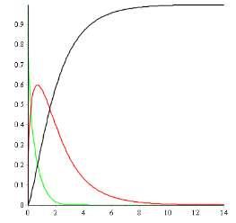
An example of simulation in Maple, is for N = 20 milion, α = 0.007/day, β = 0.65/day, d = (1/4)/day, γ = (1/5)/day, b = μN = 0.03, c1 = 0.034, c2 = 0.063, c3 = 0.046, c4 = 0.017, a = 0.0005, E(0)=30,000, I(0) = 2, R(0) = 0, V(0) = 0. We typing the following procedure into Maple, and we obtain the graph from figure 1. The graph show the evolution of the pandemic for a chosen period of time, for example of 14 days. The Maple procedure which was used is:
α:= 0.007; β:=0.65; γ:=0.2; c1:= 0.034; c2 := 0.063; c3 := 0.046; c4 := 0.017; a := 0.0005; sol:=dsolve({diff(SU(t),t)= *SU(t) *SU(t)*IN(t) , diff(E(t),t)= ( ) diff(IN(t),t)= , diff(R(t),t)= ( ) ( ) , diff(V(t),t)=a*(1 V(t)),SU(0)=0.998,E(0)=0.0015,IN(0)=0.0005,R(0)=0, V(0)=0},{SU(t),E(t),IN(t),R(t),V(t)},type=numeric,output=listprocedure): f:=subs(sol,SU(t)): g:=subs(sol,E(t)): h:=subs(sol,IN(t)): m:=subs(sol,R(t)); n:=subs(sol,V(t)); plot({f,h,m},0..14,color=[green,red,black]); .
Fig. 1 .The generalized seirv iepqa system simulation in Maple
In the first day and in the second day, the number of infected persons increase. It is displayed by the red curve. The susceptible persons have a descending trend in the green curve, while the one for recovered persons has an increasing trend in the black curve. The curve of infected people has a peak after 2 days, when their number becomes I = 0.6×2,000,000 = 1,200,000 from 2 milion.
Conclusions
Mathematical models can facilitate the improvement of the decisions making for the measures in management of an epidemic situation. Also, the elements from the fixed points theory can be used for the analysis of epidemics. Research directions for more accurate models can be more realistic compartments, higher order moment closure approximations, etc. Future research directions for our generalization would be adding subcompartments to the model, and some new parameters, such as climate type
References
[1] Abouelkheir, I., Kihal, F.El., Rachik, M. and Elmouki, I (2018). Time Needed to Control an Epidemic with Restricted Resources in SIR Model with Short Term Controlled Population: A Fixed Point Method for a Free Isoperimetric Optimal Control Problem. Math. Comput 23(64), 1 19 [2] Abreu, Z., Cantin, G. and Silva, C.J. (2021). Analysis of a COVID 19 compartmental model: a mathematical and computational approach Mathematical Biosciences and Engineering 18(6), 7979 7998
© 2022, IJASRW, All right reserve https://www.ijasrw.com
This work is licensed under a Creative Commons Attribution NonCommercial ShareAlike 4.0 International License
International Journal of Advance Study and Research Work (2581-5997)/ Volume 5/Issue 11/November 2022
[3] Area, I., Fernández, F.J., Nieto, J.J., Tojo, F.A.F. (2022) Concept and solution of digital twin based on a Stieltjes differential equations. Mathematical Methods in the Applied Sciences 45(12), 7451 7465
[4] Bauch, C.T., and Earn, D.J.D. (2004). Vaccination and the theory of games Proceedings of the National Academy of Sciences 101 (36), 13391 13394
[5] Bernoulli, D. (1766). Essai d’une nouvelle analyse de la mortalité causée par la petite vérole, et des avantages de l’inoculation pour la prévenir. [An attempt at a new analysis of the mortality caused by smallpox and of the advantages of inoculation to prevent it.] In Histoire de l’Académie royale des sciences avec les mémoires de mathématique & de physique tirez des registres de cette Académie [History of the Royal Academy of Sciences with mathematics & physics dissertations from the registers of this Academy]. 1 45
[6] Bouchnita, A., Chekroun, A., Jebrane, A. (2021). Mathematical Modeling Predicts That Strict Social Distancing Measures Would Be Needed to Shorten the Duration of Waves of COVID 19 Infections in Vietnam Front. Public Health 8:559693, 11 pages
[7] Braurer, F. (2017). Mathematical Epidemiology: Past, present, and future Infectious Disease Modelling 2(2), 113 127
[8] Bucur, A. (2021). Some Aspects About Mathematical Modeling for Epidemic Management Management of Sustainable Development 13(2), 19 28
[9] Bucur, A., Guran, L. and Petrusel, A. (2009). Fixed Point Theorems for Multivalued Operators on a Set Endowed with Vector Valued Metrics and Applications Fixed Point Theory 1, 19 34
[10] Calafiore, G.C.; Novara, C. and Possieri, C. (2020). A time varying SIRD model for the COVID 19 contagion in Italy Annual Reviews in Control. 50, 361 372
[11] Caputo, M. and Fabrizio, M. (2015). A new definition of fractional derivative without singular kernel. Progress in Fractional Differentiation and Applications. 1(2), 73 85
[12] Carcione, J.M., Santos, J.E., Bagaini, C. and Ba, J.A. (2020). Simulation of a COVID 19 Epidemic Based on a Deterministic SEIR Model. Front. Public Health 8, 230
[13] Ciesielski, K. (2007). On Stefan Banach and Some of his Results. Banach J. Math. Anal 1(1), 1 10 [14] Franke, J.E. and Yakubu, A.A. (2006). Discrete Time SIS Epidemic Model in a Seasonal Environment SIAM Journal on Applied Mathematics, 66(5), 1563 1587
[15] Giordano, G., Blanchini, F., Bruno, R. et al. (2020). Modelling the COVID 19 epidemic and implementation of population wide interventions in Italy. Nat Med 26, 855 860
[16] Hamer, W.H. (1906). On epidemic disease in England The Lancet, 167(4305), 569 574 [17] Hethcote, H.W. (2000). The mathematics of infectious disease SIAM Review, 42(4), 599 653 [18] Kermack, W.O., McKendrick, A.G. and Walker, G.T. (1927). A contribution to the mathematical theory of epidemics Proceedings of the Royal Society of London. Series A, Containing Papers of a Mathematical and Physical Character 115(772), 700 721
[19] Kirkeby, C., Brookes, V.J., Ward, M.P., Dürr, S. and Halasa, T. (2021). A Practical Introduction to Mechanistic Modeling of Disease Transmission in Veterinary Science. Front. Vet. Sci. 7, 546651 [20] Lajmanovich, A., Yorke, J.A. (1976). A deterministic model for gonorrhea in a nonhomogeneous population. Mathematical Biosciences. 28(3), 221 236
[21] Leggett, R.W. (1980). A Fixed Point Theorem with Application to an Infectious Disease Model. Journal of Mathematical Analysis and Applications 76, 91 97
[22] Liouville, J. (1837). Second mémoire sur le développement des fonctions ou parties de fonctions en séries dont divers termes sont assujettis á satisfaire a une m’eme équation différentielle du second ordre contenant un paramétre variable. J. Math. Pure et Appl 2, 16 35
[23] Liu, P. and Li, H X. (2020). Global behavior of a multi group SEIR epidemic model with age structure and spatial diffusion Mathematical Biosciences and Engineering, 17(6), 7248 7273
[24] Lucas, A.R. (2013). A fixed point theorem for a general epidemic model J. Math. Anal. Appl 404, 135 149
[25] Luo, Y.,Tang, S., Teng, Z., Zhang, I. (2019). Global dynamics in a reaction diffusion multi group SIR epidemic model with nonlinear incidence Nonlinear Analysis. Real World Applications, 50, 365 385
[26] Martcheva, M. (2015). An Introduction to Mathematical Epidemiology. New York: Springer Science+Business Media [27] Narsingani, F.J., Prajapati, M.B. and Bhathawala, P.H. (2017). Fixed Point Analysis of Kermack Mckendrick SIR Model Kalpa Publications in Computing 2, 13 19
[28] Nalawade, V.V. and Dolhare, U.P. (2016). Importance of fixed points in mathematics:a survey. International Journal of Applied and Pure Science and Agriculture. 2(12), 131 140
[29] Peter, O. J., Kumar, S., Kumari, N., Oguntolu, F.A., Oshinubi, K. and Musa, R. (2022). Transmission dynamics of Monkeypox virus: a mathematical modelling approach Modeling Earth Systems and Environment, 8(3), 3423 3434
[30] Panda, S.K. (2020). Applying fixed point methods and fractional operators in the modelling of novel coronavirus 2019 nCoV/SARS CoV 2. Results in Physics, 19, 103433
[31] van der Plank, J.E. (1963). Plant Diseases, Epidemics and Control New York: Academic Press
[32] Picard, C.É. (1890). Mémoire sur la theorie des equations aux dérivées partielles et la methode des approximations successives J. Math. Pures et Appl., 6, 145 210
[33] Pavlack, B., Grave, M., Dantas, E., Basilio, J., de La Roca, L. et al. (2021). EPIDEMIC: a didactic tool for teaching mathematical epidemiology. XL Congresso Nacional de Matemática Aplicada e Computacional (CNMAC 2021), Sep 2021, Campo Grande (virtual), Brazil hal 03338666, 8 pages
[34] Qiu, Z., Sun, Y., He, X., et al. (2022). Application of genetic algorithm combined with improved SEIR model in predicting the epidemic trend of COVID 19. China. Sci Rep 12, 8910
© 2022, IJASRW, All right reserve https://www.ijasrw.com
This work is licensed under a Creative Commons Attribution NonCommercial ShareAlike 4.0 International License
International Journal of Advance Study and Research Work (2581-5997)/ Volume 5/Issue 11/November 2022
[35] Rajapaksha, R.N.U., Wijesinghe, M.S.D., Jayasooriya, S.P., Gunawardana, B.I. and Weerasinghe, W.P.C. (2021). An Extended Susceptible Exposed Infected Recovered (SEIR) Model with Vaccination for Forecasting the COVID 19 Pandemic in Sri Lanka. medRxiv [36] Rodrigues, H.S. (2016). Application of SIR epidemiological model: new trends. International Journal of Applied Mathematics and Informatics, 10, 92 97 [37] Ross, R. (1911). The Prevention or Malaria. 2nd edn. London: Murray [38] Rus, I.A., Petrușel, A. and Sîntămărian, A. (2001). Data dependence of the fixed point set of multivalued weakly Picard operators. Studia Univ. “Babeș Bolyai”, Mathematica XLVI(2), 111 121
[39] Shaikh, A.S., Shaikh, I.N. and Nisar, K.S. (2020). A mathematical model of COVID 19 using fractional derivative: outbreak in India with dynamics of transmission and control. Adv. Differ. Equ. 373
[40] Sidi Ammi, M.R., Tahiri, M., Tilioua, M. et al. (2022). Global analysis of a time fractional order spatio temporal SIR model. Sci Rep 12, 5751 [41] Srivastava, H.M., Area, I., Nieto, J.J. (2021). Power series solution of compartmental epidemiological models. Mathematical Biosciences and Engineering 18, 3274 3290
[42] Tomar, A. and Joshi, M.C. (editors). (2021). Fixed Point Theory and its Applications to Real Word Problem. New York: Nova Science Publishers
[43] J.Xu, Y. Geng, Dynamics of a Diffusive Multigroup SVIR Model with Nonlinear Incidence, Hindawi, (2020), article ID 8847023, 15 pages
[44] Zhang, T. and Teng, Z. (2008). An impulsive delayed SEIRS epidemic model with saturation incidence. Journal of Biological Dynamics 2(1), 64 84
[45] G.F. Webb, A Reaction Diffusion Model for a Deterministic Diffusive Epidemic, J. of Mathematical Analysis and Applications, 84, (1981), 150 161f
© 2022, IJASRW, All right reserve https://www.ijasrw.com
This work is licensed under a Creative Commons Attribution NonCommercial ShareAlike 4.0 International License