
Physics
John Allum Paul MorrisPublisher's acknowledgements
IB advisers: The Publishers would like to thank the following for their advice and support in the development of this project: Arno Dirks and Aurora Vicens. We would like to offer special thanks to Paul Morris for his invaluable review and feedback during the writing process.
The Publishers would also like to thank the International Baccalaureate Organization for permission to re-use their past examination questions in the online materials.
Every effort has been made to trace all copyright holders, but if any have been inadvertently overlooked, the Publishers will be pleased to make the necessary arrangements at the first opportunity.
Although every effort has been made to ensure that website addresses are correct at time of going to press, Hodder Education cannot be held responsible for the content of any website mentioned in this book. It is sometimes possible to find a relocated web page by typing in the address of the home page for a website in the URL window of your browser.
Hachette UK’s policy is to use papers that are natural, renewable and recyclable products and made from wood grown in well-managed forests and other controlled sources. The logging and manufacturing processes are expected to conform to the environmental regulations of the country of origin.
Orders: please contact Hachette UK Distribution, Hely Hutchinson Centre, Milton Road, Didcot, Oxfordshire, OX11 7HH. Telephone: +44 (0)1235 827827. Email education@hachette.co.uk Lines are open from 9 a.m. to 5 p.m., Monday to Friday. You can also order through our website: www.hoddereducation.com ISBN: 978 1 3983 6991 7
© John Allum 2023
First published in 2012 Second edition published in 2014 This edition published in 2023 by Hodder Education, An Hachette UK Company Carmelite House 50 Victoria Embankment London EC4Y 0DZ
www.hoddereducation.com
Impression number 10 9 8 7 6 5 4 3 2 1 Year 2027 2026 2025 2024 2023
All rights reserved. Apart from any use permitted under UK copyright law, no part of this publication may be reproduced or transmitted in any form or by any means, electronic or mechanical, including photocopying and recording, or held within any information storage and retrieval system, without permission in writing from the publisher or under licence from the Copyright Licensing Agency Limited. Further details of such licences (for reprographic reproduction) may be obtained from the Copyright Licensing Agency Limited, www.cla.co.uk
Cover photo © salita2010/stock.adobe.com
Illustrations by Aptara Inc., Pantek Media and Barking Dog Art
Typeset in Times 10/14pt by DC Graphic Design Limited, Hextable, Kent Printed in Bosnia & Herzegovina
A catalogue record for this title is available from the British Library.
Tools and Inquiry
A Space, time and motion
A.1 Kinematics ........................................... 1
A .2 Forces and momentum 31
A .3 Work, energy and power ................................. 85
A .4 R igid body mechanics (HL only) 116
A.5 Relativity (HL only) 140
B The particulate nature of matter
B.1 T hermal energy transfers 176
B.2 G reenhouse effect 215
B.3 Gas laws 234
B.4 T hermodynamics (HL only) 257
B.5 Current and circuits (includes HL section) 281
C Wave behaviour
C.1 Simple harmonic motion (includes HL section) 313
C.2 Wave model ......................................... 335
C.3 Wave phenomena (includes HL section) 350
C.4 Standing waves and resonance ........................... 383
C.5 Doppler effect (includes HL section) 40 0
D Fields
D.1 G ravitational fields (includes HL section) .................... 411
D.2 Electric and magnetic fields (includes HL section) 4 42
D.3 Motion in electromagnetic fields .......................... 471
D.4 Induction (HL only) 4 87
v
Introduction vii
Contents
........................................ xi
Sample pages
E Nuclear and quantum
E.1 Structure of the atom (includes HL section) .................. 507
E.2 Quantum physics (HL only) 528
E.3 Radioactive decay (includes HL section) .................... 541
E.4 Fission 575
vi
Free online content Go to our website www.hoddereducation.com/ib-extras for free access to the following: n Practice exam-style questions for each chapter n Glossary n A nswers to self-assessment questions and practice exam-style questions n Tools and Inquiries reference guide n Internal Assessment – the scientific investigation
E.5 Fusion and stars 585 Acknowledgments .................................... 602 Index 604
Sample pages
Introduction
Welcome to Physics for the IB Diploma Third Edition, updated and designed to meet the criteria of the new International Baccalaureate (IB) Diploma Programme Physics Guide. This coursebook provides complete coverage of the new IB Physics Diploma syllabus, with first teaching from 2023. Differentiated content for SL and HL students is clearly identified throughout.
The aim of this syllabus is to integrate concepts, topic content and the nature of science through inquiry. Approaches to learning in the study of physics are integrated with the topics, along with key scientific inquiry skills. This book comprises five main themes:
l Theme A: Space, time and motion
l Theme B: The particulate nature of matter
l Theme C: Wave behaviour
l Theme D: Fields
l Theme E: Nuclear and quantum physics
Each theme is divided into syllabus topics.
The book has been written with a sympathetic understanding that English is not the first language of many students.
No prior knowledge of physics by students has been assumed, although many will have taken an earlier course (and they will find some useful reminders in the content).
In keeping with the IB philosophy, a wide variety of approaches to teaching and learning has been included in the book (not just the core physics syllabus). The intention is to stimulate interest and motivate beyond the confines of the basic physics content. However, it is very important students know what is the essential knowledge they have to take into the examination room. This is provided by the Key information boxes. If this information is well understood, and plenty of selfassessment questions have been done (and answers checked), then a student will be well-prepared for their IB Physics examination.
The online Glossary is another useful resource. It's aim is to list and explain basic terminology used in physics, but it is not intended as a list of essential information for students. Many of the terms in the Glossary are highlighted in the book as 'Key terms' and also emphasized in the nearby margins.
The ‘In cooperation with IB’ logo signifies that this coursebook has been rigorously reviewed by the IB to ensure it fully aligns with the current IB curriculum and offers high-quality guidance and support for IB teaching and learning.
vii
Sample pages
Key terms
◆ Definitions appear throughout the margins to provide context and help you understand the language of physics. There is also a glossary of all key terms online.
Common mistake
These detail some common misunderstandings and typical errors made by students, so that you can avoid making the same mistakes yourself.
How to use this book
The following features will help you consolidate and develop your understanding of physics, through concept-based learning.
Guiding questions
• T here are guiding questions at the start of every chapter, as signposts for inquiry.
• T hese questions will help you to view the content of the syllabus through the conceptual lenses of the themes.
SYLLABUS CONTENT
T his coursebook follows the order of the contents of the IB Physics Diploma syllabus.
Syllabus understandings are introduced naturally throughout each topic.
Key information
Throughout the book, you will find some content in pink boxes like this one. These highlight the essential Physics knowledge you will need to know when you come to the examination. Included in these boxes are the key equations and constants that are also listed in the IBDP Physics data booklet for the course.
Tools
The Tools features explore the skills and techniques that you require and are integrated into the physics content to be practiced in context. These skills can be assessed through internal and external assessment.
Inquiry process
The application and development of the Inquiry process is supported in close association with the Tools.
Nature of science
Nature of science (NOS) explores conceptual understandings related to the purpose, features and impact of scientific knowledge. It can be examined in Physics papers. NOS explores the scientific process itself, and how science is represented and understood by the general public. NOS covers 11 aspects: Observations, Patterns and trends, Hypotheses, Experiments, Measurements, Models, Evidence, Theories, Falsification, Science as a shared endeavour, and Global impact of science. It also examines the way in which science is the basis for technological developments and how these modern technologies, in turn, drive developments in science.
viii
Sample pages
D B
ATL ACTIVITY
Approaches to learning (ATL) activities, including learning through inquiry, are integral to IB pedagogy. These activities are contextualized through real-world applications of physics.
Content from the IBDP Physics data booklet is indicated with this icon and shown in bold. The data booklet contains electrical symbols, equations and constants that you need to familiarize yourself with as you progress through the course. You will have access to a copy of the data booklet during your examination.
Top tip!
This feature includes advice relating to the content being discussed and tips to help you retain the knowledge you need.

WORKED EXAMPLE
These provide a step-by-step guide showing you how to answer the kind of quantitative and other questions that you might encounter in your studies and in the assessment.
International mindedness is indicated with this icon. It explores how the exchange of information and ideas across national boundaries has been essential to the progress of science and illustrates the international aspects of physics.
Self-assessment questions appear throughout the chapters, phrased to assist comprehension and recall, but also to help familiarize you with the assessment implications of the command terms. These command terms are defined in the online glossary. Practice exam-style questions and their answers, together with answers to most self-assessment questions are on the accompanying website, IB Extras: www.hoddereducation.com/ib-extras
The IB learner profile icon indicates material that is particularly useful to help you towards developing in the following attributes: to be inquirers, knowledgeable, thinkers, communicators, principled, open-minded, caring, risk-takers, balanced and reflective. When you see the icon, think about what learner profile attribute you might be demonstrating – it could be more than one.
LINKING QUESTIONS
These questions are introduced throughout each topic. They are to strengthen your understanding by making connections across the themes. The linking questions encourage you to apply broad, integrating and discipline-specific concepts from one topic to another, ideally networking your knowledge. Practise answering the linking questions first, on your own or in groups. The links in this coursebook are not exhaustive, you may also encounter other connections between concepts, leading you to create your own linking questions.
TOK
Links to Theory of Knowledge (TOK) allow you to develop critical thinking skills and deepen scientific understanding by bringing discussions about the subject beyond the scope of the content of the curriculum.
ix
THEIB LEARNER PR O F EL
Sample pages
About the author
John Allum taught physics to pre-university level in international schools for more than thirty years (as a head of department). He has now retired from teaching, but lives a busy life in a mountainside village in South East Asia. He has also been an IB examiner for many years.
n Adviser, writer and reader
Paul Morris is Deputy Principal and IB Diploma Coordinator at the International School of London. He has taught IB Physics and IB Theory of Knowledge for over 20 years, has led teacher workshops internationally and has examined Theory of Knowledge. As an enthusiast for the IB concept-based continuum, Paul designed and developed Hodder Education's 'MYP by Concept' series and was author and co-author of the Physics and Sciences titles in the series. He has also advised on publishing projects for the national sciences education programmes for Singapore and Qatar.
x
Sample pages
Tools and Inquiry
Skills in the study of physics
The skills and techniques you must experience through the course are encompassed within the tools. These support the application and development of the inquiry process in the delivery of the physics course.
n Tools
l Tool 1: Experimental techniques
l Tool 2: Technology
l Tool 3: Mathematics

n Inquiry process
l Inquiry 1: Exploring and designing l Inquiry 2: Collecting and processing data l Inquiry 3: Concluding and evaluating
Throughout the programme, you will be given opportunities to encounter and practise the skills; and instead of stand-alone topics, they will be integrated into the teaching of the syllabus when they are relevant to the syllabus topics being covered.
You can see what the Tools and Inquiry boxes look like in the How to use this book section on page vi.
The skills in the study of physics can be assessed through internal and external assessment. The Approaches to learning provide the framework for the development of these skills.
Thinking skills
Tools and Inquiry xi
Social skills Communication skills Research skills Self-management skills Experimental techniques TechnologyMathematics Collecting and processing data Exploring and designing Concluding and evaluating n Figure 0.01 Tools for physics Visit the link in the QR code or this website to view the Tools and Inquiry reference guide:
Sample pages
www.hoddereducation.com/ib-extras
Tools
n Tool 1: Experimental techniques
Skill
Addressing safety of self, others and the environment
Description
• Recognize and address relevant safety, ethical or environmental issues in an investigation.
Measuring variables Understand how to accurately measure the following to an appropriate level of precision:
• Mass
• Time
• Length
• Volume
• Temperature
• Force
• Electric current
• Electric potential difference
• Angle
• Sound and light intensity
n Tool 2: Technology
Skill Description
Applying technology to collect data
• Use sensors.
• Identify and extract data from databases.
• Generate data from models and simulations.
• Carry out image analysis and video analysis of motion.
Applying technology to process data
• Use spreadsheets to manipulate data.
• Represent data in a graphical form.
• Use computer modelling.
n Tool 3: Mathematics
Skill Description
Applying general mathematics
• Use basic arithmetic and algebraic calculations to solve problems.
• Calculate areas and volumes for simple shapes.
• Carry out calculations involving decimals, fractions, percentages, ratios, reciprocals, exponents and trigonometric ratios.
• Carry out calculations involving logarithmic and exponential functions.
• Determine rates of change.
• Calculate mean and range.
• Use and interpret scientific notation (for example, 3.5 × 10⁶).
• Select and manipulate equations.
• Derive relationships algebraically.
• Use approximation and estimation.
• Appreciate when some effects can be neglected and why this is useful.
• Compare and quote ratios, values and approximations to the nearest order of magnitude.
• Distinguish between continuous and discrete variables.
xii
Sample pages
Skill
Description
• Understand direct and inverse proportionality, as well as positive and negative relationships or correlations between variables.
• Determine the effect of changes to variables on other variables in a relationship.
• Calculate and interpret percentage change and percentage difference.
• Calculate and interpret percentage error and percentage uncertainty.
• Construct and use scale diagrams.
• Identify a quantity as a scalar or vector.
• D raw and label vectors including magnitude, point of application and direction.
• D raw and interpret free-body diagrams showing forces at point of application or centre of mass as required.
• Add and subtract vectors in the same plane (limited to three vectors).
• Multiply vectors by a scalar.
• Resolve vectors (limited to two perpendicular components).
Using units, symbols and numerical values
• Apply and use SI prefixes and units.
• Identify and use symbols stated in the guide and the data booklet.
• Work with fundamental units.
• Use of units (for example, eV, eVc –2, ly, pc, h, day, year) whenever appropriate.
• Express derived units in terms of SI units.
• Check an expression using dimensional analysis of units (the formal process of dimensional analysis will not be assessed).
• Express quantities and uncertainties to an appropriate number of significant figures or decimal places.
Processing uncertainties
• Understand the significance of uncertainties in raw and processed data.
• Record uncertainties in measurements as a range (±) to an appropriate precision.
• P ropagate uncertainties in processed data in calculations involving addition, subtraction, multiplication, division and raising to a power.
• Express measurement and processed uncertainties—absolute, fractional (relative) and percentage—to an appropriate number of significant figures or level of precision.
Graphing
• Sketch graphs, with labelled but unscaled axes, to qualitatively describe trends.
• Construct and interpret tables, charts and graphs for raw and processed data including bar charts, histograms, scatter graphs and line and curve graphs.
• Construct and interpret graphs using logarithmic scales.
• Plot linear and non-linear graphs showing the relationship between two variables with appropriate scales and axes.
• D raw lines or curves of best fit.
• D raw and interpret uncertainty bars.
• Extrapolate and interpolate graphs.
• Li nearize graphs (only where appropriate).
• O n a best-fit linear graph, construct lines of maximum and minimum gradients with relative accuracy (by eye) considering all uncertainty bars.
• Determining the uncertainty in gradients and intercepts.
• I nterpret features of graphs including gradient, changes in gradient, intercepts, maxima and minima, and areas under the graph.
Tools and Inquiry xiii
Sample pages
Inquiry process
n Inquiry 1: Exploring and designing
Skill
Exploring
Description
• Demonstrate independent thinking, initiative and insight.
• Consult a variety of sources.
• Select sufficient and relevant sources of information.
• Formulate research questions and hypotheses.
• St ate and explain predictions using scientific understanding.
Designing
• Demonstrate creativity in the designing, implementation and presentation of the investigation.
• Develop investigations that involve hands-on laboratory experiments, databases, simulations and modelling.
• Identify and justify the choice of dependent, independent and control variables.
• Justify the range and quantity of measurements.
• Design and explain a valid methodology.
• Pilot methodologies.
Controlling variables Appreciate when and how to:
• calibrate measuring apparatus, including sensors
• maintain constant environmental conditions of systems
• i nsulate against heat loss or gain
• reduce friction
• reduce electrical resistance
• t ake background radiation into account.
n Inquiry 2: Collecting and processing data
Skill Description
Collecting data
• Identify and record relevant qualitative observations.
• Collect and record sufficient relevant quantitative data.
• Identify and address issues that arise during data collection.
Processing data
Interpreting results
• Carry out relevant and accurate data processing.
• I nterpret qualitative and quantitative data.
• I nterpret diagrams, graphs and charts.
• Identify, describe and explain patterns, trends and relationships.
• Identify and justify the removal or inclusion of outliers in data (no mathematical processing is required).
• Assess accuracy, precision, reliability and validity.
n Inquiry 3: Concluding and evaluating
Skill
Concluding
Description
• I nterpret processed data and analysis to draw and justify conclusions.
• Compare the outcomes of an investigation to the accepted scientific context.
• Relate the outcomes of an investigation to the stated research question or hypothesis.
• Discuss the impact of uncertainties on the conclusions.
Evaluating
• Evaluate hypotheses.
• Identify and discuss sources and impacts of random and systematic errors.
• Evaluate the implications of methodological weaknesses, limitations and assumptions on conclusions.
• Explain realistic and relevant improvements to an investigation.
xiv
Sample pages
Kinematics A.1
◆ K inematics Study of motion.
◆ Classical physics Physics theories that pre-dated the paradigm shifts introduced by quantum physics and relativity.
◆ Uniform Unchanging.
◆ Magnitude Size.
◆ Scalars Quantities that have only magnitude (no direction).
◆ Vector A quantity that has both magnitude and direction.
Guiding questions
• How can the motion of a body be described quantitatively and qualitatively?
• How can the position of a body in space and time be predicted?
• How can the analysis of motion in one and two dimensions be used to solve real-life problems?
Kinematics is the study of moving objects. In this topic we will describe motion by using graphs and equations, but the causes of motion (forces) will be covered in the next topic, A.2 Forces and Momentum. The ideas of classical physics presented in this chapter can be applied to the movement of all masses, from the very small (freely moving atomic particles) to the very large (stars).
8 m s–1
N W E S stationary observer
velocity, car
20 m
Figure A1.1 Describing the position and motion of a car
To completely describe the motion of an object at any one moment we need to state its position, how fast it is moving, the direction in which it is moving and whether its motion is changing. For example, we might observe that a car is 20 m to the west of an observer and moving northeast with a constant (uniform) velocity of 8 m s−1. See Figure A1.1.
Of course, any or all, of these quantities might be changing. In real life the movement of many objects can be complicated; they do not often move in straight lines and they might even rotate or have different parts moving in different directions.
In this chapter we will develop an understanding of the basic principles of kinematics by dealing first with objects moving in straight lines, and calculations will be confined to those objects that have a uniform (unchanging) motion.
Tool 3: Mathematics
Identify a quantity as a scalar or a vector
Everything that we measure has a magnitude and a unit.
For example, we might measure the mass of a book to be 640 g. Here, 640 g is the magnitude (size) of the measurement, but mass has no direction.
Quantities that have only magnitude, and no direction, are called scalars.
All physical quantities can be described as scalars or vectors.
Quantities that have both magnitude and direction are called vectors.
For example, force is a vector quantity because the direction in which a force acts is important. Most quantities are scalars. Some common examples of scalars used in physics are mass, length, time, energy, temperature and speed.
However, when using the following quantities, we need to know both the magnitude and the direction in which they are acting, so they are vectors:
l displacement (distance in a specified direction) l velocity (speed in a given direction) l force (including weight)
l acceleration l momentum and impulse l f ield strength (gravitational, electric and magnetic).
In diagrams, all vectors are shown with straight arrows, pointing in a certain direction from the correct point of application.
The lengths of the arrows are proportional to the magnitudes of the vectors.
A.1 Kinematics 1
Sample pages
◆ Distance Total length travelled, without consideration of directions.
◆ Displacement, linear Distance in a straight line from a fixed reference point in a specified direction.
Distance and displacement
SYLLABUS CONTENT
T he motion of bodies through space and time can be described and analysed in terms of position, velocity and acceleration.
T he change in position is the displacement.
T he difference between distance and displacement.
The term distance can be used in different ways, for example we might say that the distance between New York City and Boston is 300 k m, meaning that a straight line between the two cities has a length of 300 k m. Or, we might say that the (travel) distance was 348 k m, meaning the length of the road between the cities.
We will define distance as follows:
Distance (of travel) is the total length of a specified path between two points. SI unit: metre, m
◆ Metre, m SI unit of length (fundamental). South Station, Boston, MA Port Authority Bus Terminal, New York
In physics, displacement (change of position) is often more important than distance: The displacement of an object is the distance in a straight line from a fixed reference point in a specified direction.
Continuing the example given above, if a girl travels from New York to Boston, her displacement will be 300 k m to the northeast (see Figure A1.2).
384km 300km
Both distance and displacement are given the symbol s and the SI unit metres, m. Kilometres, km, centimetres, cm, and millimetres, mm, are also in widespread use. We often use the symbol h for heights and x for small displacements.
Figure A1.3 shows the route of some people walking around a park. The total distance walked was 4 km, but the displacement from the reference point varied and is shown every few minutes by the vector arrows (a – e). The final displacement was zero because the walkers returned to their starting place.
Speed and velocity
SYLLABUS CONTENT
start and end here
e
Figure A1.2 Boston is a travel distance of 384 k m and a displacement of 300 k m northeast from New York City a b c d
Velocity is the rate of change of position. T he difference between instantaneous and average values of velocity, speed and acceleration, and how to determine them.
Speed
Figure A1.3 A walk in the park
The displacement of Wellington from Auckland, New Zealand, is 494 k m south (Figure A1.4). The road distance is 642 k m and it is predicted that a car journey between the two cities will take 9.0 hours.
Theme A: Space, time and motion
2
Sample pages
If we divide the total distance by the total time (642 / 9.0) we determine a speed of 71 k m h−1. In this example it should be obvious that the speed will have changed during the journey and the calculated result is just an average speed for the whole trip. The value seen on the speedometer of the car is the speed at any particular moment, called the instantaneous speed
◆ Speed, v Average speed = distance travelled/time taken. Instantaneous speed is determined over a very short time interval, during which it is assumed that the speed does not change.
◆ Reaction time The time delay between an event occurring and a response. For example, the delay that occurs when using a stopwatch.
◆ Sensor An electrical component that responds to a change in a physical property with a corresponding change in an electrical property (usually resistance). Also called a transducer.
◆ Light gate Electronic sensor used to detect motion when an object interrupts a beam of light.
Tool 1: Experimental techniques
Understand how to accurately measure quantities to an appropriate level of precision: time
Accurate time measuring instruments are common, but the problem with obtaining accurate measurements of time is starting and stopping the timers at exactly the right moments.
Whenever we use stopwatches or timers operated by hand, the results will have an unavoidable and variable uncertainty because of the delays between seeing an event and pressing a button to start or stop the timer. The delay between seeing something happen and responding with some kind of action is known as reaction time. For example, for car drivers it is usually assumed that a driver takes about 0.7 s to press the brake pedal after they have seen a problem. (But some drivers will be able to react quicker than this.) A car will travel about 14 m in this time if it is moving at 50 km h−1. Reaction times will increase if the driver is distracted, tired, or under the influence of any type of drug, such as alcohol.
A simple way of determining a person’s reaction time is by measuring how far a metre ruler falls before it can be caught between thumb and finger (see Figure A1.5). The time, t, can then be calculated using the equation for distance, s = 5t2 (explained later in this topic).
If the distance the ruler falls s = 0.30
Rearranging for t, t = s 5 = 0.30 5
So, reaction time t = 0.25 s.
Under these conditions a typical reaction time is about 0.25 s, but it can vary considerably depending on the conditions involved. The measurement can be repeated with the person tested being blindfolded to see if the reaction time changes if the stimulus (to catch the ruler) is either sound or touch, rather than sight.
In science experiments it is sensible to make time measurements as long as possible to decrease the effect of this problem. (This reduces the percentage uncertainty.) Repeating measurements and calculating an average will also reduce the effect of random uncertainties. If a stopwatch is started late because of the user’s reaction time, it may be offset by also stopping the stopwatch late for the same reason.
Electronics sensors, such as light gates, are very useful in obtaining accurate time measurements. See below.
A.1 Kinematics 3
Figure A1.5 Determining reaction time
Auckland
494km 642km
Wellington
Sample pages
Figure A1.4 Distance and displacement from Auckland to Wellington
Figure A1.6 Measuring speed in a laboratory
There are a number of different methods in which speed can be measured in a school or college laboratory. Figure A1.6 shows one possibility, in which a glider is moving on a frictionless air track at a constant velocity. The time taken for a card of known length (on the glider) to pass through the light gate is measured and its speed can be calculated from length of card / time taken.
Use sensors
glider
Tool 2: Technology
An electronic sensor is an electronic device used to convert a physical quantity into an electrical signal. The most common sensors respond to changes in light level, sound level, temperature or pressure.
A light gate contains a source of light that produces a narrow beam of light directed towards a sensor on the other side of a gap. When an object passes across the light beam, the unit behaves as a switch which turns a timer on or off very quickly.
◆ Second, s SI unit of time (fundamental).
Tool 3: Mathematics
Determine rates of change
The Greek capital letter delta, Δ, is widely used in physics and mathematics to represent a change in the value of a quantity.
For example, Δ x = (x2 – x1), where x2 and x1 are two different values of the variable x
The change involved is often considered to be relatively small.
Most methods of determining speed involve measuring the small amount of time (Δt) taken to travel a certain distance (Δ s). The SI unit for time is the second, s.
speed = distance travelled time taken (SI unit m s –1)
This calculation determines an average speed during time Δt, but if Δt is small enough, we may assume that the calculated value is a good approximation to an instantaneous speed.
Speed is a scalar quantity. Speed is given the same symbol, (v), as velocity.
Figure A1.7 The peregrine falcon is reported to be the world’s fastest animal (speeds measured up to 390 k m h−1)
Theme A: Space, time and motion

4
air track
light gate
Sample pages
◆ At rest Stays stationary in the same position.
◆ Mi lky Way The galaxy in which our Solar System is located.
Nature of science: Observations
Objects at rest
It is common in physics for people to refer to an object being at rest, meaning that it is not moving. But this is not as simple as it may seem. A stone may be at rest on the ground, meaning that it is not moving when compared with the ground: it appears to us to have no velocity and no acceleration. However, when the same stone is thrown upwards, at the top of its path its instantaneous speed may be zero, but it has an acceleration downwards.
We cannot assume that an object which is at rest has no acceleration; its velocity may be changing –either in magnitude, in direction, or both.
We may prefer to refer to an object being stationary, suggesting that an object is not moving over a period of time.
Of course, the surface of the Earth is moving, the Earth is orbiting the Sun, which orbits the centre of the Milky Way galaxy, which itself exists in an expanding universe. So, at a deeper level, we must understand that all motion is relative and nowhere is truly stationary. This is the starting point for the study of Relativity (Topic A.5).
Velocity
◆ Velocity, v Rate of change of position.
Velocity, v, is the rate of change of position. It may be considered to be speed in a specified direction. velocity, v = displacement time taken = Δ s Δt (SI unit m s –1)
The symbol Δ s represents a change of position (displacement).
Velocity is a vector quantity. 12 m s−1 is a speed. 12 m s−1 to the south is a velocity. We use positive and negative signs to represent velocities in opposite directions. For example, +12 m s−1 may represent a velocity upwards, while −12 m s−1 represents the same speed downwards, but we may choose to reverse the signs used.
Speed and velocity are both represented by the same symbol (v) and their magnitudes are calculated in the same way (v = Δ s Δt ) with the same units. It is not surprising that these two terms are sometimes used interchangeably and this can cause confusion. For this reason, it may be better to define these two quantities in words, rather than symbols.
As with speed, we may need to distinguish between average velocity over a time interval, or instantaneous velocity at a particular moment. As we shall see, the value of an instantaneous velocity can be determined from the gradient of a displacement–time graph.
Top tip!
When a direction of motion is clearly stated (such as ‘up’, ‘to the north’, ‘to the right’ and so on), it is very clear that a velocity is being discussed. However, we may commonly refer to the ‘velocity’ of a car, for example, without stating a direction. Although this is casual, it is usually acceptable because an unchanging direction is implied, even if it is not specified. For example, we may assume that the direction of the car is along a straight road.
A.1 Kinematics 5
Sample pages
WORKED EXAMPLE A1.1
A satellite moves in circles along the same path around the Earth at a constant distance of 6.7 × 10³ k m from the Earth’s centre. Each orbit takes a time of 90 minutes.
a Calculate the average speed of the satellite. b Describe the instantaneous velocity of the satellite.
c Determine its displacement from the centre of the Earth after i 360 minutes ii 405 minutes.
Answer
a v = circumference time for orbit = 2πr Δt = (2 × π × 6.7 × 10⁶) (90 × 60) = 7.8 × 10³ m s –1
b The velocity also has a constant magnitude of 7.8 × 10³ m s−1, but its direction is continuously changing. Its instantaneous velocity is always directed along a tangent to its circular orbit. See Figure A1.8.
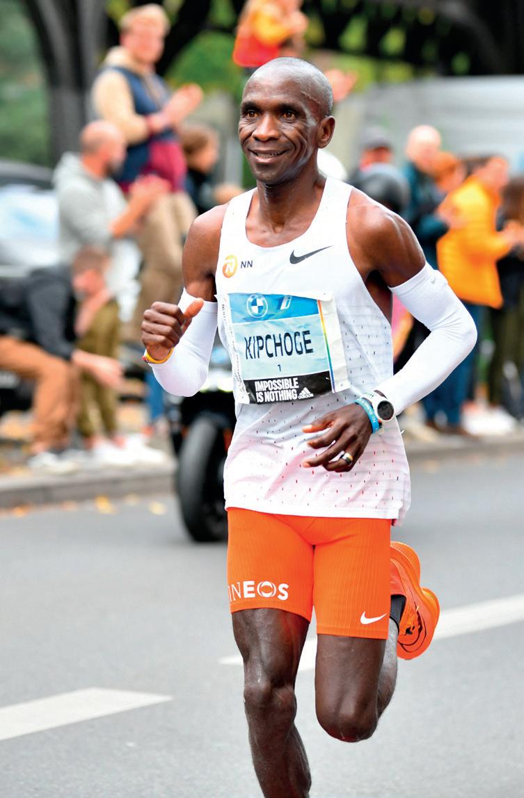
1 Calculate the average speed (m s−1) of an athlete who can run a marathon (42.2 k m) in 2 hours, 1 minute and 9 seconds. (The men’s world record at the time of writing.)
Figure A1.9 Eliud Kipchoge, world record holder for the men’s marathon
v
◆ Orbit The curved path (may be circular) of a mass around a larger central mass.
◆ Tangent Line which touches a given curve at a single point.
Figure A1.8 Satellite’s instantaneous velocity
c i 360 minutes is the time for four complete orbits. The satellite will have returned to the same place. Its displacement from the centre of the Earth compared to 360 minutes earlier will be the same. (But the Earth will have rotated.)
ii I n the extra 45 minutes the satellite will have travelled half of its orbit. It will be on the opposite side of the Earth’s centre, but at the same distance. We could represent this as −6.7 × 10³ k m from the Earth’s centre.
2 A small ball dropped from a height of 2.0 m takes 0.72 s to reach the ground.
a Calculate 2.0 0.72
b W hat does your answer represent?
c The speed of the ball just before it hits the ground is 5.3 m s−1. This is an instantaneous speed. Distinguish between an instantaneous value and an average value. d State the instantaneous velocity of the ball just before it hits the ground.
e After bouncing, the ball only rises to a lower height. Give a rough estimate of the instantaneous velocity of the ball as it leaves the ground.
3 A magnetic field surrounds the Earth and it can be detected by a compass. State whether it is a scalar or a vector quantity. Explain your answer.
4 On a flight from Rome to London, a figure of 900 k m h−1 is displayed on the screen.
a State whether this is a speed or a velocity. b Is it an average or instantaneous value?
c Convert the value to m s−1
d Calculate how long it will take the aircraft to travel a distance of 100 m
Theme A: Space, time and motion
6
Sample pages
◆ Acceleration, a Rate of change of velocity with time. Acceleration is a vector quantity.
◆ Deceleration Term commonly used to describe a decreasing speed.
Acceleration
SYLLABUS CONTENT
Acceleration is the rate of change of velocity.
Motion with uniform and non-uniform acceleration.
Any variation from moving at a constant speed in a straight line is described as an acceleration
Going faster, going slower and/or changing direction are all different kinds of acceleration (changing velocities).
When the velocity (or speed) of an object changes during a certain time, the symbol u is used for the initial velocity and the symbol v is used for the final velocity. These velocities are not necessarily the beginning and end of the entire motion, just the velocities at the start and end of the period of time that is being considered.
Acceleration, a, is defined as the rate of change of velocity with time: a = Δv Δt = (v – u) t (SI unit m s –2)
One way to determine an acceleration is to measure two velocities and the time between the measurements. Figure A1.10 shows an example.
light gate
glider
air track
Figure A1.10 Measuring two velocities to determine an acceleration
Acceleration is a vector quantity. For a typical motion in which displacement and velocity are both given positive values, a positive acceleration means increasing speed in the same direction (+Δv), while a negative acceleration means decreasing speed in the same direction (−Δv). In everyday speech, a reducing speed is often called a deceleration
For a motion in which displacement and velocity are given negative values, a positive acceleration means a decreasing speed. For example, a velocity change from –6 m s−1 to –4 m s−1 in 0.5 s corresponds to an acceleration:
a = Δv Δt = ([–4]–[–6]) 0.5 = + 4 ms –2
As with speed and velocity, we may need to distinguish between average acceleration over a time interval, or instantaneous acceleration at a particular moment.
A.1 Kinematics 7
Sample pages
WORKED EXAMPLE A1.2
A high-speed train travelling with a velocity of 84 m s−1 needs to slow down and stop in a time of one minute.
a Determine the necessary average acceleration.
b Calculate the distance that the train will travel in this time assuming that the acceleration is uniform.
Answer
a a = Δv Δt = (0 – 84) 60 = –1.4 m s –2
T he acceleration is negative. The negative sign shows that the velocity is decreasing.
b average speed = (84 – 0) 2 = 42 m s –1
distance = average speed × time = 42 × 60 = 2.5 × 10³ m
5 A car moving at 12.5 m s−1 accelerates uniformly on a straight road at a rate of 0.850 m s−2
a Calculate its velocity after 4.60 s.
b W hat uniform rate of acceleration will reduce the speed to 5.0 m s−1 in a further 12 s?
6 A n athlete accelerates uniformly from rest at the start of a race at a rate of 4.3 m s−2 . How much time is needed before her speed has reached 8.0 m s−1?
7 A trolley takes 3.62 s to accelerate from rest uniformly down a slope at a rate of 0.16 m s−2 . A light gate at the bottom of the slope records a velocity of 0.58 m s−1. What was the speed about halfway down the slope, 1.2 s earlier?
Inquiry 1: Exploring and designing
Designing
Suppose that the Principal of your school or college is worried about safety from traffic on the nearby road. He has asked your physics class to collect evidence that he can take to the police. He is concerned that the traffic travels too fast and that the vehicles do not slow down as they approach the school.
1 Using a team of students, working over a period of one week, with tape measures and stop watches, develop an investigation which will produce sufficient and accurate data that can be given in a report to the Principal. Explain how you would ensure that the investigation was carried out safely.
2 W hat is the best way of presenting a summary of this data?
◆ Linear relationship
One which produces a straight line graph.
Tool 3: Mathematics
Interpret features of graphs
In order to analyse and predict motions we have two methods: graphical and algebraic. Firstly, we will look at how motion can be represented graphically.
Graphs can be drawn to represent any motion and they provide extra understanding and insight (at a glance) that very few of us can get from written descriptions or equations. Furthermore, the gradients of graphs and the areas under graphs often provide additional useful information.
Displacement–time graphs and distance–time graphs
Displacement–time graphs, similar to those shown in Figure A1.11, show how the displacements of objects from a known reference point vary with time. All the examples shown in Figure A1.11 are straight lines and are representing linear relationships and constant velocities.
l Line A represents an object moving away from the reference point (zero displacement) such that equal displacements occur in equal times. That is, the object has a constant velocity.
Theme A: Space, time and motion
8
THEIB LEARNER PR O F EL
Sample pages
C
A
Any linear displacement–time graph represents a constant velocity (it does not need to start or end at the origin).
D
l Line B represents an object moving with a greater velocity than A.
l Line C represents an object that is moving back towards the reference point.
C
l Line D represents an object that is stationary (at rest). It has zero velocity and stays at the same distance from the reference point.
0 0 0 0 0 0
s t Time, t Time, t
Figure A1.12 shows how we can represent displacements in opposite directions from the same reference point.
Displacement, s Displacement, s intervals
D t Time, t Time, t
Displacement, s
C
The solid line represents the motion of an object moving with a constant (positive) velocity. The object moves towards a reference point (where the displacement is zero), passes it, and then moves away from the reference point with the same velocity. The dotted line represents an identical speed in the opposite direction (or it could also represent the original motion if the directions chosen to be positive and negative were reversed).
0 0 0 0
D Time, t Time, t
Displacement, s Displacement, s equal time intervals equal changes in displacement A B 0 0
Any curved (non-linear) line on a displacement–time graph represents a changing velocity, in other words, an acceleration. This is illustrated in Figure A1.13. 0 Displacement, s Time, t
a B Displacement, s Displacement, s Time, t 0
Figure A1.12 Motion in opposite directions represented on a displacement–time graph
A
C
b D Time, t 0 0 0
Figure A1.13 Accelerations on displacement–time graphs
20
Figure A1.11 Constant velocities on displacement–time graphs a Displacement/m Time/s
Figure A1.13a shows motion away from a reference point. Line A represents an object accelerating. Line B represents an object decelerating. Figure A1.13b shows motion towards a reference point. Line C represents an object accelerating. Line D represents an object decelerating. The values of the accelerations represented by these graphs may, or may not, be constant. (This cannot be determined without a more detailed analysis.)
0
40 024
20
In physics, we are usually more concerned with displacement–time graphs than distance–time graphs. In order to explain the difference, consider Figure A1.14.
0
b Distance/m Time/s
Figure A1.14a shows a displacement–time graph for an object thrown vertically upwards with an initial speed of 20 m s−1 (without air resistance). It takes 2 s to reach a maximum height of 20 m. At that point it has an instantaneous velocity of zero, before returning to where it began after 4 s and regaining its initial speed. Figure A1.14b is a less commonly used graph showing how the same motion would appear on an overall distance–time graph.
20
40 024 Time/s 024
b Distance/m Time/s
Tool 3: Mathematics
Interpret features of graphs: gradient
0
40 024
Figure A1.14 a Displacement–time and b distance–time graphs for an object moving up and then down
In this topic we will need to repeatedly use the following information: l T he gradient of a displacement–time graph equals velocity. l T he gradient of a velocity–time graph equals acceleration. In the following section we will explore how to measure and interpret gradients.
A.1 Kinematics 9
s s
Sample pages
Gradients of displacement–time graphs
Displacement/m
20 2 8
Δs Δt 0 0
Consider the motion at constant velocity represented by Figure A1.15.
8
Displacement/m Time/s
The gradient of the graph = Δ s Δt , which is the velocity of the object. A downwards sloping graph would have a negative gradient (velocity).
In this example, constant velocity, v = Δ s Δt = (20 – 8.0) (8.0 – 2.0) = 2.0 m s –1
Figure A1.16 represents the motion of an object with a changing velocity, that is, an accelerating object.
18 Δt
3
0 5 t1 t2 t3 0
Figure A1.16 Finding an instantaneous velocity from a curved displacement–time graph
◆ Gradient The rate at which one physical quantity changes in response to changes in another physical quantity. Commonly, for an y –x graph, gradient = Δy Δ x
s 23
Time/s
The gradient of this graph varies, but at any point it is still equal to the velocity of the object at that moment, that is, the instantaneous velocity. The gradient (velocity) can be determined at any time by drawing a tangent to the curve, as shown.
The triangle used to calculate the gradient should be large, in order to make this process as accurate as possible. In this example: velocity at time t2 = (18 – 3.0) (23 – 5.0) = 0.83 m s –1
A tangent drawn at time t1 would have a smaller gradient and represent a smaller velocity. A tangent drawn at time t3 would represent a larger velocity.
Figure A1.15 Finding a constant velocity from a displacement–time graph We have been referring to the object's displacement and velocity, although no direction has been stated. This is acceptable because that information would be included when the origin of the graph was explained. If information was presented in the form of a distance–time graph, the gradient would represent the speed.
In summary:
The gradient of a displacement–time graph represents velocity. The gradient of a distance–time graph represents speed.
WORKED EXAMPLE A1.3
c Calculate the maximum speed of the train. d Determine the average speed of the train.
Answer
3000
2000
Figure A1.17 represents the motion of a train on a straight track between two stations. a Describe the motion. b State the distance between the two stations. 0 0
4000 50100150200250 Time/s
a T he train started from rest. For the first 90 s the train was accelerating. It then travelled with a constant speed until a time of 200 s. After that, its speed decreased to become zero after 280 s b 3500 m
1000
Distance/m 300
Figure A1.17 Distance–time graph for train on a straight track
c From the steepest, straight section of the graph: v = Δ s Δt = (3000 – 800) (200 – 90) = 20 m s –1
d average speed = total distance travelled time taken = 3500 300 = 11.7 m s–1
Theme A: Space, time and motion
10
Sample pages
C
8 Draw a displacement–time graph for a swimmer swimming a total distance of 100 m at a constant speed of 1.0 m s−1 in a swimming pool of length 50 m
9 Describe the motion of a runner as shown by the graph in Figure A1.18.
Displacement 0 T ime
Figure A1.18 Displacement–time graph for a runner
10 Sketch a displacement–time graph for the following motion: a stationary car is 25 m away; 2 s later it starts to move further away in a straight line from you with a constant acceleration of 1.5 m s−2 for 4 s; then it continues with a constant velocity for another 8 s
equal changes in velocity
–3 –2 –1 0 1 2 3 4 5 Displacement/cm
11 Figure A1.19 is a displacement–time graph for an object. 23 AB 45678 1 T ime/s –4 –5
Figure A1.19 A displacement–time graph for an object
a Describe the motion represented by the graph in Figure A1.19.
b Compare the velocities at points A and B.
c W hen is the object moving with its maximum and minimum velocities?
d Estimate values for the maximum and minimum velocities.
e Suggest what kind of object could move in this way.
Velocity–time graphs and speed–time graphs
D
v t Time, t Time, t
Velocity, v Velocity, v equal time intervals
Figure A1.20, shows how the velocity of four objects changed with time. Any straight (linear) line on any velocity–time graph shows that equal changes of velocity occur in equal times – that is, it represents constant acceleration.
C
l Line A shows an object that has a constant positive acceleration.
0 0 0 0 0 0
l Line B represents an object moving with a greater positive acceleration than A.
l Line C represents an object that has a negative acceleration.
Velocity, v Velocity, v intervals
A 0 0
l Line D represents an object moving with a constant velocity – that is, it has zero acceleration. Curved lines on velocity–time graphs represent changing accelerations.
Velocity, v
A B 0 0 0 0
C
D t Time, t Time, t
D Time, t Time, t
Figure A1.20
Constant accelerations on velocity–time graphs
Velocities in opposite directions are represented by positive and negative values. We will return to the example shown in Figure A1.14 to illustrate the difference between velocity–time and speed–time graphs. Figure A1.21a shows how the speed of an object changes as it is thrown up in the air (without air resistance), reaches its highest point, where its speed has reduced to zero, and then returns downwards. Figure A1.21b shows the same information in terms of velocity. Positive velocity represents motion upwards, negative velocity represents motion downwards. In most cases, the velocity graph is preferred to the speed graph. 0 0
a
a
b
b
Speed + Velocity
0 0
Figure A1.21 a Speed–time and b velocity–time graphs for an object thrown upwards.
moving up moving down highest point Time Time 0
Speed + Velocity − Velocity
moving up moving down highest point Time Time 0
A.1 Kinematics 11
Sample pages
Gradients of velocity–time graphs
Consider the motion at constant acceleration shown by the straight line in Figure A1.22. 0 0
Velocity/m s 1 Δv Δt
12 4 9 Time/s
7
Figure A1.22 Finding the gradient of a velocity–time graph
The gradient of the graph = Δv Δt , which is equal to the acceleration of the object. In this example, the constant acceleration: a = Δv Δt = (12.0 – 7.0) (9.0 – 4.0) = + 1.0 m s –2
The acceleration of an object is equal to the gradient of the velocity–time graph. A changing acceleration will appear as a curved line on a velocity–time graph. A numerical value for the acceleration at any time can be determined from the gradient of the graph at that moment. See Worked example A1.4.
WORKED EXAMPLE A1.4
Velocity/m s 1
10
The red line in Figure A1.23 shows an object decelerating (a decreasing negative acceleration). Use the graph to determine the instantaneous acceleration at a time of 10.0 s 5
15 101520 25 0 0 Time/s
5
Figure A1.23 Finding an instantaneous acceleration from a velocity–time graph
Answer
Using a tangent to the curve drawn at t = 10 s.
Acceleration, a = Δv Δt = (0 – 12) (22 – 0) = –0.55 m s –2
The negative sign indicates a deceleration. In this example the large triangle used to determine the gradient accurately was drawn by extending the tangent to the axes for convenience.
Theme A: Space, time and motion
12
Sample pages
Tool 3: Mathematics
Interpret features of graphs: areas under the graph
The area under many graphs has a physical meaning. As an example, consider Figure A1.24a, which shows part of a speed–time graph for a vehicle moving with constant acceleration. The area under the graph (the shaded area) can be calculated from the average speed, given by (v1 + v 2) 2 , multiplied by the time, Δt.
The area under the graph is therefore equal to the distance travelled in time Δt. In Figure A1.24b a vehicle is moving with a changing (decreasing) acceleration, so that the graph is curved, but the same rule applies – the area under the graph (shaded) represents the distance travelled in time Δt.
The area in Figure A1.24b can be estimated in a number of different ways, for example by counting small squares, or by drawing a rectangle that appears (as judged by eye) to have the same area. (If the equation of the line is known, it can be calculated using the process of integration, but this is not required in the IB course.)
◆ Integration
a Δt
In the following section, we will show how a change in displacement can be calculated from a velocity–time graph.
a Δt
Speed, v 0 0
v1
0 0
v2 Time, t
Speed, v 0 0
b Speed, v 0 0
v2 Time, t
v1
Mathematical process used to determine the area under a graph.
Speed, v
b Δt Time, t
Figure A1.24 Area under a speed–time graph for a constant acceleration and b changing acceleration
Areas under velocity–time and speed–time graphs
As an example, consider again Figure A1.22. The change of displacement, Δ s, between the fourth and ninth seconds can be found from (average velocity) × time. Δ s = (12.0 + 7.0) 2 × (9.0 – 4.0) = 47.5 m
This is numerically equal to the area under the line between t = 4.0 s and t = 9.0 s (as shaded in Figure A1.22). This is always true, whatever the shape of the line.
The area under a velocity–time graph is always equal to the change of displacement. The area under a speed–time graph is always equal to the distance travelled.
As an example, consider Figure A1.21a. The two areas under the speed–time graph are equal and they are both positive. Each area equals the vertical height travelled by the object. The total area = total distance = twice the height. Each area under the velocity graph also represents the height, but the total area is zero because the areas above and below the time axis are equal, indicating that the final displacement is zero – the object has returned to where it started.
A.1 Kinematics 13
Sample pages
12
8
6
4
Velocity/m s 1 20 0
10 4 6 8 10
Figure A1.25 shows a velocity–time graph for an athlete running 100 m in 10.0 s. The area under the curve is equal to 100 m and it equals the area under the dotted line. (The two shaded areas are judged by sight to be equal.) The initial acceleration of the athlete is very important, and in this example, it is about 5 m s−2
2
Figure A1.25 Velocity–time graph for an athlete running 100 m
Time/s
Figure A1.26 Elaine Thompson-Herah (Jamaica) won the women’s 100 m in the Tokyo Olympics in 2021 in a time of 10.54 s

12 Look at the graph in Figure A1.27.
a Describe the straight-line motion represented by the graph.
b Calculate accelerations for the three parts of the journey.
c W hat was the total distance travelled? d W hat was the average velocity?
4.0
3.0
2.0
1.0
Velocity/m s 1 567 8 43210 0
Time/s
Figure A1.27
Velocity–time graph
13 The velocity of a car was read from its speedometer at the moment it started and every 2 s afterwards. The successive values (converted to m s−1) were: 0, 1.1, 2.4, 6.9, 12.2, 18.0, 19.9, 21.3 and 21.9.
a Draw a graph of these readings.
b Use the graph to estimate i the maximum acceleration ii the distance covered in 16 s
14 Look at the graph in Figure A1.28.
a Describe the straight-line motion of the object represented by the graph.
b Calculate the acceleration during the first 8 s
c W hat was the total distance travelled in 12 s?
d W hat was the total displacement after 12 s?
e What was the average velocity during the 12 s interval?
Velocity/m s 1 0 4 8 12 16 16 12 8 4 2 4 6 8 10 12 14
Time/s
Figure A1.28 Velocity–time graph
15 Sketch a velocity–time graph of the following motion: a car is 100 m away and travelling along a straight road towards you at a constant velocity of 25 m s−1 Two seconds after passing you, the driver decelerates uniformly and the car stops 62.5 m away from you.
Velocity/m s 1
a Velocity/m s 1 b 10
5 43210 0 Time/s
25
20
15
20
15
16 Figure A1.29 shows how the velocity of a car, moving in a straight line, changed in the first 5 s after starting. Use the area under the graph to show that the distance travelled was about 40 m 5
25 5 43210 0 Time/s
10
Figure A1.29 Determining the displacement of a car during acceleration
Theme A: Space, time and motion
14
Sample pages
Tool 2: Technology
Use spreadsheets to manipulate data
Figure A1.30 represents how the velocities of two identical cars changed from the moment that their drivers saw danger in front of them and tried to stop their cars as quickly as possible. It has been assumed that both drivers have the same reaction time (0.7 s) and both cars decelerate at the same rate (−5.0 m s−2).
The distance travelled at constant velocity before the driver reacts and depresses the brake pedal is known as the ‘thinking distance’. The distance travelled while decelerating is called the ‘braking distance’. The total stopping distance is the sum of these two distances.
Car B, travelling at twice the velocity of car A, has twice the thinking distance. That is, the thinking distance is proportional to the velocity of the car. The distance travelled when braking, however, is proportional to the velocity squared. This can be confirmed from the areas under the v–t graphs. The area under graph B is four times the area under graph A (during the deceleration). This has important implications for road safety and most countries make sure that people learning to drive must understand how stopping distances change with the vehicle’s velocity. Some countries measure the reaction times of people before they are given a driving licence.
Set up a spreadsheet that will calculate the total stopping distance for cars travelling at initial speeds, u, between 0 and 40 m s−1 with a deceleration of −6.5 m s−2. (Make calculations every 2 m s−1.) The thinking distance can be calculated from s t = 0.7u (reaction time 0.7 s).
In this example the braking time can be calculated from: t b = u 6.5 and the braking distance can be calculated from: s b = (u 2)t b
◆ Spreadsheet (computer) Electronic document in which data is arranged in the rows and columns of a grid, and can be manipulated and used in calculations.
Velocity/m s –1
20
15
10
A
Figure A1.30 Velocity–time graphs for two cars braking
Use the data produced to plot a computer-generated graph of stopping distance ( y -axis) against initial speed (x-axis). 0 0
25 12
Acceleration–time graphs
5
B 345 Time/s
In this topic, we are mostly concerned with constant accelerations. The graphs in Figure A1.31 show five straight lines representing constant accelerations. A changing acceleration would be represented by a curved line on the graph. a 0
+ t A
B C
a 0
D + t
a 0
Figure A1.31 Graphs of constant acceleration
E
+ t
l Line A shows zero acceleration, constant velocity.
l Line B shows a constant positive acceleration (uniformly increasing velocity).
l Line C shows the constant negative acceleration (deceleration) of an object that is slowing down at a uniform rate.
l Line D shows a (linearly) increasing positive acceleration.
l Line E shows an object that is accelerating positively, but at a (linearly) decreasing rate.
A.1 Kinematics 15
Sample pages
Areas under acceleration–time graphs
Figure A1.32 shows the constant acceleration of a moving car.
Acceleration/m s 2 5 0 0
1.5 13
Using a = Δv Δt , between the fifth and thirteenth seconds, the velocity of the car increased by:
Δv = aΔt = 1.5 × (13.0 – 5.0) = 12 m s−1
Δt
Time/s
Figure A1.32 Calculating change of velocity from an acceleration–time graph
The change in velocity is numerically equal to the area under the line between t = 5 s and t = 13 s (the shaded area in Figure A1.32). This is always true, whatever the shape of the line.
The area under an acceleration–time graph is equal to the change of velocity.
17 Draw an acceleration–time graph for a car that starts from rest, accelerates at 2 m s−2 for 5 s, then travels at constant velocity for 8 s, before decelerating uniformly to rest again in a further 2 s
18 Figure A1.33 shows how the acceleration of a car changed during a 6 s interval. If the car was travelling at 2 m s−1 after 1 s, estimate a suitable area under the graph and use it to determine the approximate speed of the car after another 5 s.
19 Sketch displacement–time, velocity–time and acceleration–time graphs for a bouncing ball that was dropped from rest. Continue the sketches until the third time that the ball contacts the ground.
◆ Calculus Branch of mathematics which deals with continuous change.
◆ Differentiate Mathematically determine an equation for a rate of change.
TOK Mathematics and the arts
THEIB LEARNER PR O EL
4.0
3.0
2.0
1.0 0
5.0 Acceleration/m s –2 0246 Time/s
Figure A1.33 Acceleration–time graph for an accelerating car
l W hy is mathematics so important in some areas of knowledge, particularly the natural sciences?
If you study Mathematics: Analysis and Approaches (SL or HL) or Mathematics: Applications and Interpretations (HL) you will explore how calculus is used to mathematically describe changing functions. The gradient of a function is found using the process of differentiation and the area under a curve is found using the process of integration. The mathematical procedures for calculus were developed by Isaac Newton and he first published his ‘method of fluxions’ as an appendix to his book Opticks in 1704. Newton is usually therefore credited with the ‘invention’ of calculus – although historians of science point to the earlier work of Gottfried Wilhelm Leibniz, published in 1684. Newton accused Leibniz of plagiarism, even though Leibniz’s work was published first! In fact, it is Leibniz’s notation that we still use today. So, who invented calculus?
Theme A: Space, time and motion
16
Sample pages
◆ Equations of motion
Equations that can be used to make calculations about objects that are moving with uniform acceleration.
Equations of motion for uniformly accelerated motion
SYLLABUS CONTENT
The equations of motion for solving problems with uniformly accelerated motion as given by: s = (u + v) 2 t v = u + at s = ut + 1 2at2 v 2 = u 2 + 2as
The five quantities u, v, a, s and t are all that is needed to fully describe the motion of an object that is moving with uniform acceleration.
l u = velocity (speed) at the start of time t
l v = velocity (speed) at the end of time t l a = acceleration (constant)
l s = displacement occurring in time t
l t = time taken for velocity (speed) to change from u to v and to travel a distance s
If any three of the quantities are known, the other two can be calculated using the first two equations highlighted below.
If we know the initial velocity u and the uniform acceleration a of an object, then we can determine its final velocity v after a time t by rearranging the equation used to define acceleration: a = (v – u) t
D B
This gives: v = u + at
If an object moving with velocity u accelerates uniformly to a velocity v, then its average velocity is: (u + v) 2
LINKING QUESTION
l How are the equations for rotational motion related to those for linear motion?
This question links to understandings in Topic A.4.
Then, since distance = average velocity × time: s = (u + v) 2 t
D B
These two equations can be combined mathematically to give two further equations, shown below. These very useful equations do not involve any further physics theory, they just express the same physics principles in a different way.
s = ut + 1 2 at2 v 2 = u2 + 2as
D B
A.1 Kinematics 17
Sample pages
WORKED EXAMPLE A1.5
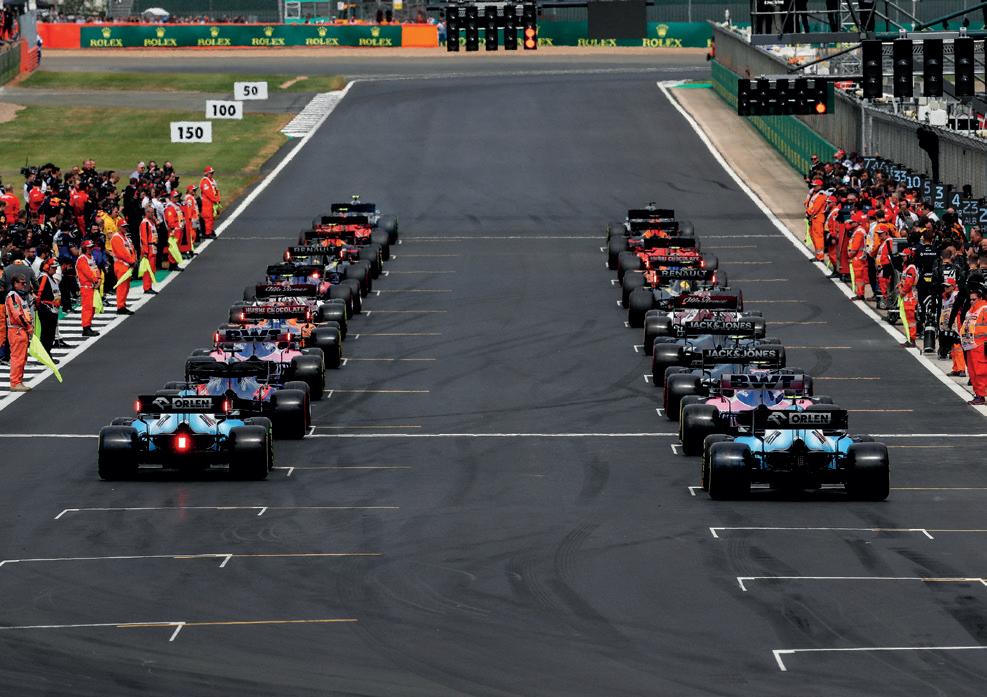
A Formula One racing car (see Figure A1.34) accelerates from rest at 18 m s−2
a Calculate its speed after 3.0 s
b Calculate how far it travels in this time.
c If it continues to accelerate at the same rate, determine its velocity after it has travelled 200 m f rom the start.
Answer
a v = u + at = 0 + (18 × 3.0) = 54 m s−1
b s = (u + v) 2 t = (0 + 54) 2 × 30 = 81 m
But note that the distance can be calculated directly, without first calculating the final velocity, as follows: s = ut + 1 2at2 = (0 × 3.0) + (0.5 × 18 × 3.02) = 81 m
c v 2 = u2 + 2as = 02 + (2 × 18 × 200) = 7200 v = 85 m s−1
WORKED EXAMPLE A1.6
A train travelling at 50 m s−1 (180 km h−1) needs to decelerate uniformly so that it stops at a station 2.0 kilometres away.
a Determine the necessary deceleration.
b Calculate the time needed to stop the train.
Answer
a v 2 = u2 + 2as 02 = 502 + (2 × a × 2000) a = −0.63 m s−2 b v = u + at 0 = 50 + (−0.63) × t t = 80 s
Alternatively, you could use s = (u + v) 2 t
In the following questions, assume that all accelerations are uniform.
20 A ball rolling down a slope passes a point P with a velocity of 1.2 m s−1. A short time later it passes point Q with a velocity of 2.6 m s−1 .
a W hat was its average velocity between P and Q?
b If it took 1.4 s to go from P to Q, determine the distance PQ.
c Calculate the acceleration of the ball.
21 A n aircraft accelerates from rest along a runway and takes off with a velocity of 86.0 m s−1. Its acceleration during this time is 2.40 m s−2
a Calculate the distance along the runway that the aircraft needs to travel before take-off.
b Predict how long after starting its acceleration the aircraft takes off.
Theme A: Space, time and motion
18
Figure A1.34 Formula One racing cars at the starting grid
Sample pages
22 A n ocean-going cruiser can decelerate no quicker than 0.0032 m s−2 .
24 A car travelling at a constant velocity of 21 m s−1 (faster than the speed limit of 50 km h−1) passes a stationary police car. The police car accelerates after the other car at 4.0 m s−2 for 8.0 s and then continues with the same velocity until it overtakes the other car.
a W hen did the two cars have the same velocity?
b Determine if the police car has overtaken the other car after 10 s
c By equating two equations for the same distance at the same time, determine exactly when the police car overtakes the other car.
Figure A1.35 Ocean-going cruise liner

a Determine the minimum distance needed to stop if the ship is travelling at 10 knots. (1 knot = 0.514 m s−1)
b How much time does this deceleration require?
23 A n advertisement for a new car states that it can travel 100 m from rest in 8.2 s
a Discuss why the car manufacturers express the acceleration in this way (or the time needed to reach a certain speed).
b Calculate the average acceleration.
c Calculate the velocity of the car after this time.
25 A car brakes suddenly and stops 2.4 s later, after travelling a distance of 38 m a Calculate its deceleration. b W hat was the velocity of the car before braking?
26 A spacecraft travelling at 8.00 k m s−1 accelerates at 2.00 × 10⁻³ m s−2 for 100 hours. a How far does it travel during this acceleration? b W hat is its final velocity?
27 Combine the first two equations of motion (given on page 17) to derive the second two equations: v 2 = u2 + 2as s = ut + 1 2 at2
Acceleration due to gravity
The motions of objects through the air are common events and deserve special attention.
At the start, we will consider only objects that are moving vertically up, or down, under the effects of gravity only. That is, we will assume (to begin with) that air resistance has no significant effect.
◆ A ir resistance Resistive force opposing the motion of an object through air. A type of drag force.
When an object held up in the air is released from rest, it will accelerate downwards because of the force of gravity. Figure A1.36 shows a possible experimental arrangement that could be used to determine a value for this acceleration.
Collecting data
s
ruler electromagnet steel ball timer trapdoor
Figure A1.36 An experiment to measure the acceleration due to gravity
Inquiry 2: Collecting and processing data
Figure A1.36 shows how the time for a steel ball to fall a certain distance can be determined experimentally.
Describe how this apparatus can be used to collect and record sufficient, relevant quantitative data which will enable an accurate value for the acceleration of free fall to be determined from a suitable graph.
A.1 Kinematics 19
Sample pages
◆ Acceleration due to gravity, g Acceleration of a mass falling freely towards Earth. On, or near the Earth’s surface, g = 9.8 ≈ 10 m s−2 . Also called acceleration of free fall
◆ Free fall Motion through the air under the effects of gravity but without air resistance.
◆ Negligible Too small to be significant.
In the absence of air resistance, all objects (close to the Earth’s surface) fall towards the Earth with the same acceleration, g = 9.8 m s−2
g is known as the acceleration of free fall due to gravity (sometimes called acceleration due to free fall).
g is not a true constant. Its value varies very slightly at different locations around the world. Although, to 2 significant figures (9.8) it has the same value everywhere on the Earth’s surface. A convenient value of g = 10 m s−2 is commonly used in introductory physics courses.
The acceleration of free fall ( g) reduces with distance from the Earth. (For example, at a height of 100 k m above the Earth’s surface the value of g is 9.5 m s−2.) We will return to this subject in Topic D.1.
WORKED EXAMPLE A1.7
A ball is dropped vertically from a height of 18.3 m. Assuming that the acceleration of free fall is 9.81 m s−2 and air resistance is negligible, calculate:
a its velocity after 1.70 s b its height after 1.70 s c its velocity when it hits the ground d the time for the ball to reach the ground.
Answer
a v = u + at = 0 + (9.81 × 1.70) = 16.7 m s –1 b s = ut + 1 2at2 = 0 + (1 2 × 9.81 × 1.702) = 14.2 m
So, height above ground = (18.3 – 14.2) = 4.1 m c v 2 = u2 + 2as = 02 + (2 × 9.81 × 18.3) = 359 v = 18.9 m s−1 d v = u + at 18.9 = 0 + (9.81 × t) t = 1.93 s
Tool 3: Mathematics
Appreciate when some effects can be neglected and why this is useful
When studying physics, you may be advised to make assumptions when answering numerical questions. For example: ‘assume that air resistance is negligible / is insignificant’. It is possible that this is a true statement, for example, air resistance will have no noticeable effect on a solid rubber ball falling 50 cm to the ground. However, the usual reason for advising you to ignore an effect is to make the calculation simpler, and not go beyond what is required in your course.
Calculating the time for a table-tennis ball dropped 50 cm to the ground will result in an underestimate if air resistance is ignored, but the answer can be interpreted as a lower limit to the time taken, and you may be questioned on your understanding of that. Other examples will be found in all topics. Examples include: assuming friction between surfaces is negligible (Topic A.2); assuming thermal energy losses are negligible (Topic B.1); assuming the internal resistance of a battery is negligible (Topic B.5).
Theme A: Space, time and motion
20
D
Sample pages
B
Moving up and down
If gravity is the only force acting, all objects close to the Earth's surface have the same acceleration (9.8 m s−2 downwards), whatever their mass and whether they are moving down, moving up or moving sideways.
The velocity of an object moving freely vertically downwards will increase by 9.8 m s−1 every second. The velocity of an object moving freely vertically upwards will decrease by 9.8 m s−1 every second.
Top tip!
Displacement, velocity and acceleration are all vector quantities and the signs used for motions up and down can be confusing.
If displacement measured up from the ground is considered to be positive, then the acceleration due to gravity is always negative. Velocity upwards is positive, while velocity downwards is negative.
If displacement measured down from the highest point is considered to be positive, then the acceleration due to gravity is always positive. Velocity upwards is negative, while velocity downwards is positive.
positive velocity
negative velocity displacement positive
acceleration negative acceleration positive
Figure A1.37 Directions of vectors
WORKED EXAMPLE A1.8
displacement positive
velocity negative OR
greatest height velocity positive
A ball is thrown vertically upwards and reaches a maximum height of 21.4 m. For the following questions, assume that g = 9.81 m s –2
a Calculate the speed with which the ball was released.
b State any assumption that you made in answering a
c Determine where the ball will be 3.05 s after it was released.
d Calculate its velocity at this time.
Answer
a v 2 = u2 + 2as
02 = u2 + (2 × [−9.81] × 21.4)
u2 = 419.9
u = 20.5 m s−1
I n this example, the vector quantities directed upwards (u, v, s) are considered positive and the quantity directed downwards (a) is negative. The same answer would be obtained by reversing all the signs.
b It was assumed that there was no air resistance.
c s = ut + 1 2at2 = (20.5 × 3.05) + (1 2 × [–9.81] × 3.052)
s = +16.9 m (above the ground)
d v = u + at = 20.5 + (−9.81 × 3.05) = −9.42 m s−1 (moving downwards)
A.1 Kinematics 21
Sample pages
In the following questions, ignore the possible effects of air resistance.
Use g = 9.81 m s−2 .
28 Discuss possible reasons why the acceleration due to gravity is not exactly the same everywhere on or near the Earth’s surface.
29 a How long does it take a stone dropped from rest from a height of 2.1 m to reach the ground?
b If the stone was thrown downwards with an initial velocity of 4.4 m s−1, calculate the speed with which it hits the ground.
c If the stone was thrown vertically upwards with an initial velocity of 4.4 m s−1, with what speed would it hit the ground?
30 A small rock is thrown vertically upwards with an initial velocity of 22 m s−1
a Calculate when its velocity will be 10 m s−1
b Explain why there are two possible answers to a
Projectile motion
SYLLABUS CONTENT
31 A falling ball has a velocity of 12.7 m s−1 as it passes a window 4.81 m above the ground.
Predict when the ball will hit the ground.
32 A ball is thrown vertically upwards with a velocity of 18.5 m s−1 from a window that is 12.5 m above the ground.
a Determine when it will pass the same point moving down.
b With what velocity will it hit the ground?
c Calculate how far above the ground the ball was after exactly 2.00 s.
33 Two balls are dropped from rest from the same height. If the second ball is released 0.750 s after the first, and assuming they do not hit the ground, calculate the distance between the balls: a 3.00 s after the second ball was dropped b 2.00 s later.
34 A stone is dropped from rest from a height of 34 m Another stone is thrown downwards 0.5 s later. If they both hit the ground at the same time, show that the second stone was thrown with a velocity of 5.5 m s−1
◆ Projectile An object that has been projected through the air and which then moves only under the action of the forces of gravity and air resistance.
◆ Resolve (a vector) To express a single vector as components (usually two components which are perpendicular to each other).
T he behaviour of projectiles in the absence of fluid resistance, and the application of the equations of motion resolved into vertical and horizontal components.
T he qualitative effect of fluid resistance on projectiles, including time of flight, trajectory, velocity, acceleration, range and terminal speed.
In our discussion of objects moving through the air, we have so far only considered motion vertically up or down. Now we will extend that work to cover objects moving in any direction. A projectile is an object that has been projected through the air (for example: fired, launched, thrown, kicked or hit) and which then moves only under the action of the force of gravity (and air resistance, if significant). A projectile has no ability to power or control its own motion.
Tool 3: Mathematics
Resolve vectors
This process occurs in several places during the course, but the most prominent examples are resolving velocities (as below) and forces.
Components of a projectile’s velocity
The instantaneous velocity of a projectile at any time can conveniently be resolved into vertical and horizontal components, v V and v H, as shown in Figure A1.38.
Theme A: Space, time and motion
22
Sample pages
Common mistake
When using these equations make sure that the angle θ is the angle between the velocity and the horizontal.
vertical component of velocity
vV = v sin θ θ
velocity of projectile, v horizontal component of velocity
vH = v cos θ
D B
◆ Stroboscope Apparatus used for observing rapid motions. It produces regular flashes of light at an appropriate frequency chosen by the user.
◆ Trajectory Path followed by a projectile.
◆ Parabolic In the shape of a parabola. The trajectory of a projectile is parabolic in a gravitational field if air resistance is negligible.
◆ Range (of a projectile) Horizontal distance travelled before impact with the ground.
Figure A1.38 Vertical and horizontal components of velocity
Vertical and horizontal components of velocity, v:
v V = v sin θ v H = v cos θ
WORKED EXAMPLE A1.9
A tennis player strikes the ball so that it leaves the racket with a velocity of 64.0 m s−1 at an angle of 6.0° below the horizontal. Calculate the vertical and horizontal components of this velocity.
Answer
v H = v cos θ = 64.0 × cos 6.0 = 64 m s−1 (63.649... seen on calculator display)
v V = v sin θ = 64.0 × sin 6.0 = 6.7 m s−1 downwards
Figure A1.39 A tennis player serving a ball
Components perpendicular to each other can be analysed separately
The vertical and horizontal components of velocity can be treated separately (independently) in calculations.
l Earlier in this topic, we stated that any object (close to the Earth's surface) which is affected only by gravity (no air resistance) will accelerate towards the Earth with an acceleration of 9.8 m s−2. This remains true even if the object is projected sideways (so that its velocity has a horizontal component).
l If there is no air resistance, the horizontal component of a projectile’s velocity will remain constant (until it comes into contact with something else).
Figure A1.40 shows a stroboscopic picture of a bouncing ball. The time intervals between each image of the ball are all the same.
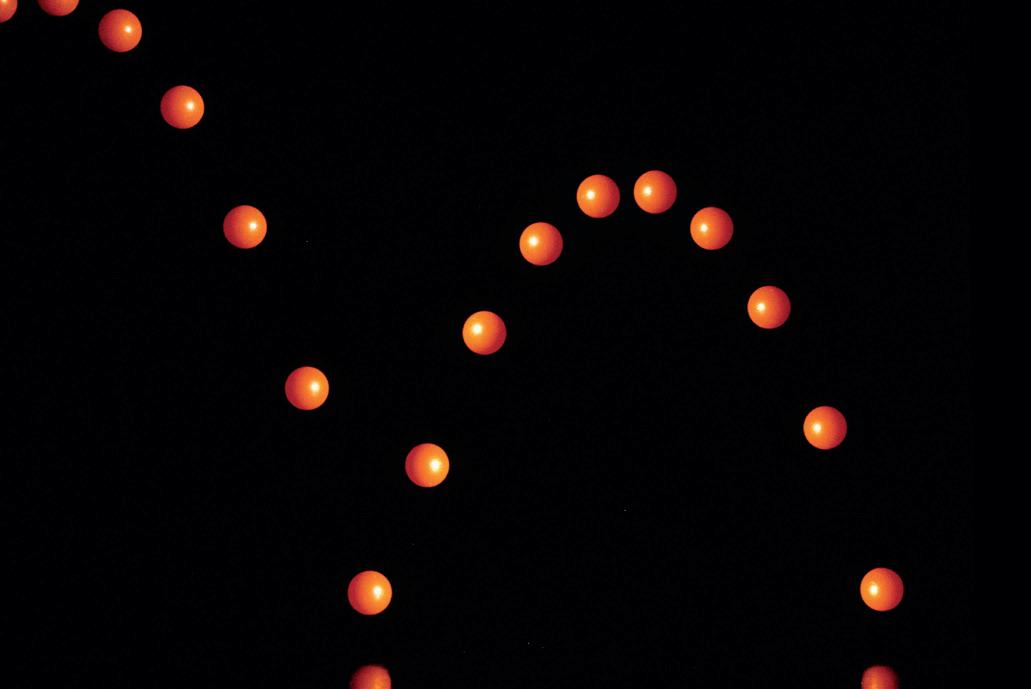
The horizontal separations of successive images of the ball are all the same because the horizontal component of velocity is constant. The vertical separations of successive images of the ball increase as the ball accelerates as it falls, and the separations decrease as the ball decelerates as it moves upwards after bouncing on the ground.
Figure A1.40 Parabolic trajectory of a bouncing ball
The path followed by a projectile (as seen in Figure A1.40) is called its trajectory. The typical shape of a freely moving projectile is parabolic. The horizontal distance covered is called the range of the projectile.
A.1 Kinematics 23
Sample pages
initial horizontal velocity
object projected horizontally
object dropped vertically
Figure A1.41 compares the trajectory of an object dropped vertically to the trajectory of an object projected horizontally at the same time. Note that both objects fall equal distances in the same time. This is true whatever the horizontal component of velocity (assuming negligible air resistance)
WORKED EXAMPLE A1.10
Object projected horizontally
A bullet was fired horizontally with a speed of 524 m s−1 from a height of 22.0 m above the ground. Calculate where it hit the ground. Assume that air resistance was negligible.
Answer
Figure A1.41 The parabolic trajectory of an object projected horizontally compared with an object dropped vertically
First, we need to calculate how long the bullet is in the air. We can do this by finding the time that the same bullet would have taken to fall to the ground if it had been dropped vertically from rest (so u = 0): s = ut + 1 2at2
22.0 = 0 + (0.5 × 9.81 × t2) t = 2.12 s
Without air resistance the bullet will continue to travel with the same horizontal component of velocity (524 m s−1) until it hits the ground 2.12 s later. Therefore: horizontal distance travelled = horizontal velocity × time horizontal distance = 524 × 2.12 = 1.11 × 10³ m (1.11 k m)
ATL A1A: Thinking skills
Providing a reasoned argument to support conclusions
Figure A1.42 shows an experimental arrangement in which a steel ball can be projected horizontally from a table top. Sketch a graph to show the pattern of results that you would expect to see when the range x was measured for different heights, h. Explain your reasoning.
table top h x
projectilepath
◆ Impact Collision involving relatively large forces over a short time.
Figure A1.42 Investigating range, x, travelled by a projectile
WORKED EXAMPLE A1.11
Object projected at an angle to the horizontal
A stone was thrown upwards from a height 1.60 m above the ground with a speed of 18.0 m s−1 at an angle of 52.0° to the horizontal. Assuming that air resistance is negligible, calculate: a its maximum height b the vertical component of velocity when it hits the ground c the time taken to reach the ground d the horizontal distance to the point where it hits the ground e the velocity of impact.
Theme A: Space, time and motion
24
Sample pages
Top tip!
If we know the velocity and position of a projectile, we can always use its vertical component of velocity to determine: l the time taken before it reaches its maximum height, and the time before it hits the ground l the maximum height reached (assuming its velocity has an upwards component).
The horizontal component can then be used to determine the range.
Answer
First, we need to know the two components of the initial velocity:
v V= v sin θ = 18.0 sin 52.0° = 14.2 m s−1
v H= v cos θ = 18.0 cos 52.0° = 11.1 m s−1
a Using v 2 = u2 + 2as for the upwards vertical motion (with directions upwards considered to be positive), and remembering that at the maximum height v = 0, we get: 0 = 14.22 + [2 × (−9.81) × s]
s = +10.3 m above the point from which it was released; a total height of 11.9 m.
b Using v 2 = u2 + 2as for the complete motion gives: v 2 = 14.22 + [2 × (−9.81) × (−1.60)]
v = 15.27 = 15.3 m s−1 downwards
c Using v = u + at gives: –15.27 = 14.2 + (−9.81)t t = 3.00 s
d Using s = vt with the horizontal component of velocity gives: s = 11.1 × 3.00 = 33.3 m
vi 18.0 m s–1 14.2 m s–1
1.6 m
10.3 m 11.1 m s–1
Figure A1.43 Object projected at an angle to the horizontal
15.3 m s–1
e Figure A1.43 illustrates the information we have so far, and the unknown angle, θ, and velocity, v i 52° θ 11.1 m s–1 33.3 m
From looking at the diagram (Figure A1.43), we can use Pythagoras’s theorem to calculate the velocity of impact. (velocity of impact)2 = (horizontal component)2 + (vertical component)2
vi 2 = 11.12 + 15.32
vi = 18.9 m s−1
T he angle of impact with the horizontal, θ, can be found using trigonometry: tan θ = 15.3 11.1
θ = 54.0°
A.1 Kinematics 25
Sample pages
◆ Imagination Formation of new ideas that are not related to direct sense perception or experimental results.
◆ Intuition Immediate understanding, without reasoning.
◆ Inspiration Stimulation (usually to be creative).
TOK
The natural sciences
l W hat is the role of imagination and intuition in the creation of hypotheses in the natural sciences?
The independence of horizontal and vertical motion in projectile motion may seem unexpected and counterintuitive. It requires imagination (some would say genius) to propose ideas and theories which are contrary to accepted wisdom and ‘common sense’. This is especially true in understanding the worlds of relativity and quantum physics, where relying on everyday experiences for inspiration is of little or no use.
It is worth remembering that many of the well-established concepts and theories of classical physics that are taught now in introductory physics lessons would have seemed improbable to many people at the time they were first proposed. For example, many people would say (incorrectly) that a force is needed to keep an object moving at constant speed (see Topic A.2).
Fluid resistance and terminal speed
So far, we have only considered projectile motion in which air resistance is negligible. We will now broaden the discussion.
◆ Drag Force(s) opposing motion through a fluid; sometimes called fluid resistance.
◆ F luid Liquid or gas.
◆ Fluid resistance (friction) Force(s) opposing motion through a fluid; sometimes called drag.
As any object moves through air, the air is forced to move out of the path of the object. This causes a force opposing the motion called air resistance, also known as drag. Drag forces will oppose the motion of an object moving in any direction through any gas or liquid. (Gases and liquids are both described as fluids because they can flow.) Such forces opposing motion are generally described as fluid resistance
Figure A1.44 gives a visual impression of air resistance. It shows the movement of air (marked by streamers) past a model of a car. (The picture was taken in a wind tunnel, in which moving air was directed towards the vehicle.)
Figure A1.44 Air flow over a clay aerodynamic model of a high-performance sports vehicle
Theme A: Space, time and motion
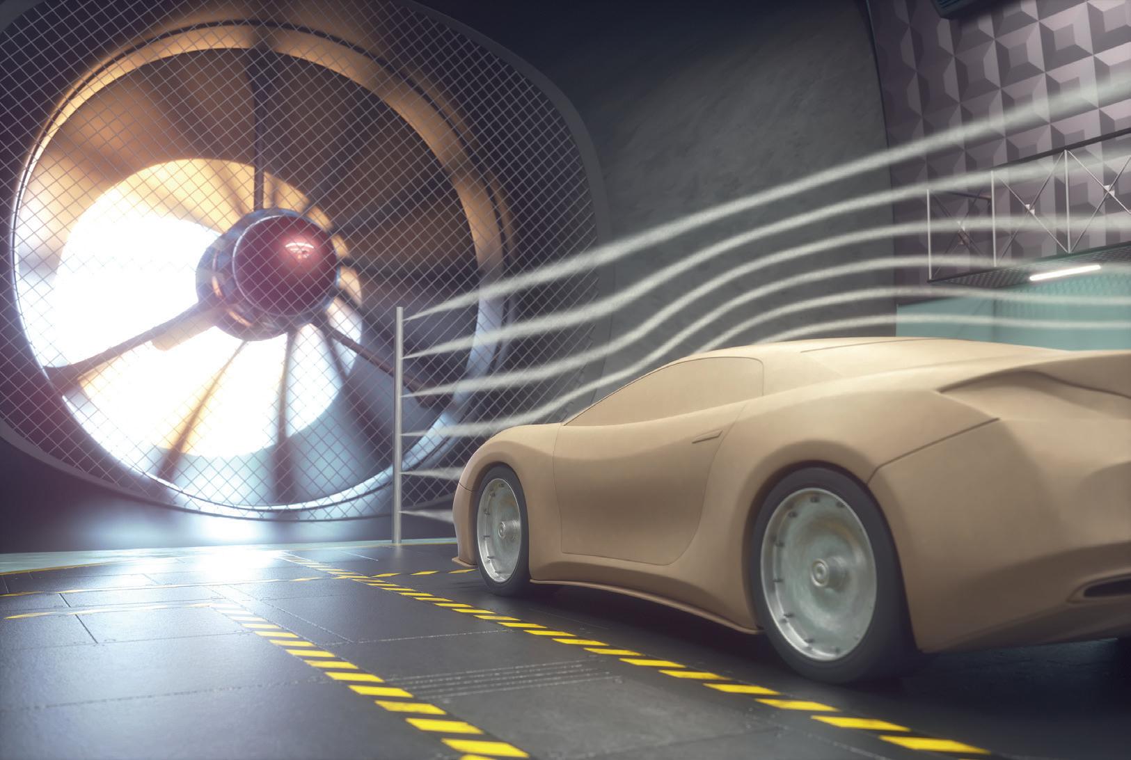
26
Sample pages
Figure A1.45 An example of a graph of velocity against time for an object falling under the effect of gravity, with (B) and without (A) air resistance
◆ Terminal speed (velocity) The greatest downwards speed of a falling object that is experiencing resistive forces (for example, air resistance). It occurs when the object’s weight is equal to the sum of resistive forces (+ upthrust).
Top tip!
The concept of a top (terminal) speed can also be applied to the horizontal motion of vehicles, like trains, cars and aircraft. As they travel faster, increasing air resistance reduces their acceleration to zero.
Figure A1.45 represents the motion of an object falling towards Earth.
Line A shows the motion without air resistance and with a constant acceleration of 9.8 m s−2 (≈ 10). Line B shows the motion more realistically, with air resistance.
When any object first starts to fall, there is no air resistance. As the object falls faster, the air resistance increases, so that the rate of increase in velocity becomes less. This is shown in the Figure A1.45 by line B becoming less steep. Eventually the object reaches a constant, maximum speed known as the terminal speed or terminal velocity (‘terminal’ means final).
Objects falling through fluids (such as air) have a maximum speed, called terminal speed, which occurs when their acceleration has reduced to zero because of increasing fluid resistance (as their velocity increases).
The value of an object’s terminal speed will depend on its cross-sectional area, shape and weight, as discussed in Topic A.2. The terminal speed of skydivers (Figure A1.46) is usually quoted at about 200 km h−1 (56 m s−1).
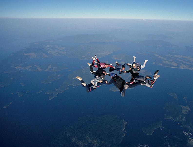
Terminal speed also depends on the density of the air. In October 2012 Felix Baumgartner (Figure A1.47), an Austrian skydiver, reached a world record speed of 1358 k m h−1 by starting his jump from a height of about 39 km above the Earth’s surface, where the density of air is about 250 times less than near the Earth’s surface. In 2014 Alan Eustace completed a jump from greater altitude, but at 1323 k m h−1 he did not break Baumgartner’s speed record.
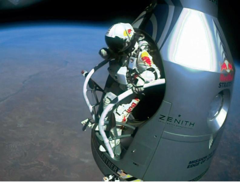
Effect of fluid (air) resistance on projectiles
without air resistance with air resistance
Without air resistance we assume that the horizontal component of a projectile’s velocity is constant, but with air resistance it decreases. Without air resistance the vertical motion always has a downwards acceleration of 9.8 m s−2, but with air resistance the acceleration will be reduced for falling objects and the deceleration increased for objects moving upwards.
Figure A1.48 shows typical trajectories with and without air resistance (for the same initial velocity).
Figure A1.48 Effect of air resistance on the trajectory of a projectile
Air resistance reduces the range of a projectile and its trajectory will not be parabolic.
A.1 Kinematics 27
Figure A1.46 Skydivers at their terminal speed
Figure A1.47 Felix Baumgartner about to jump from a height of 39 k m
v /m s –1
05101520 50 100 150 200 0 A B
terminal speed t /s
Sample pages
◆ Video analysis Analysis of motion by freeze-frame or slow-motion video replay.
Tool 2: Technology
Carry out image analysis and video analysis of motion
Video-capture technology is used in sports, such as tennis and soccer. Capturing the trajectory of a projectile on video allows us to analyse its motion frame-by-frame. For example, the cameras used in VAR in football usually capture 50 frames per second, so the motion of the projectile (the ball) can be observed at time intervals of 0.02 s.
Explain how you could use video analysis of motion to investigate the motion of a shuttlecock in a game of badminton.

Figure A1.49
In the following questions, ignore the possible effects of air resistance. Use g = 9.81 m s−2 .
35 At an indoor rifle range, a bullet was fired horizontally at the centre of a target 36 m away. If the speed of the bullet was 310 m s−1, predict where the bullet will strike the target.
36 Repeat Worked example A1.11 for a stone thrown with a velocity of 26 m s−1 at an angle of 38° to the horizontal from a cliff top. The point of release was 33 m vertically above the sea.
37 It can be shown that the maximum theoretical range of a projectile occurs when it is projected at an angle of 45° to the ground (once again, ignoring the effects of air resistance). Calculate the maximum distance a golf ball will travel before hitting the ground if its initial velocity is 72 m s−1. (Because you need to assume that there is no air resistance, your answer should be much higher than the actual ranges achieved by top-class golfers. Research to determine the actual ranges achieved in competition golf.)
38 A jet of water from a hose is aimed directly at the base of a flower, as shown in Figure A1.50. The water emerges from the hose with a speed of 3.8 m s−1 a Calculate the vertical and horizontal components of the initial velocity of the water. b How far away from the base of the plant does the water hit the ground? 0.84 m θ 2.0 m
Figure A1.50 Water from a hose aimed at the base of a flower
39 If the maximum distance a man can throw a ball is 78 m, what is the minimum speed of release of the ball? (Assume that the ball lands at the same height from which it was thrown and that the greatest range for a given speed is when the angle is 45°.)
Theme A: Space, time and motion
28
Consider how video analysis could be used to investigate the motion of a badminton shuttlecock.
THEIB LEARNER PR O EL
Sample pages
40 Figure A1.51 shows a player making a basketball shot.
a In practice, air resistance can be considered negligible for a basketball. Suggest a reason why.
b Make a copy of the figure and add to it two other possible trajectories which will result in the ball arriving at the basket.
c Suggest which trajectory is best and explain your reasoning.
d Add to your drawing a possible trajectory that would enable a light-weight sponge ball to reach the basket.
Figure A1.51 Basketball player making a shot
Nature of science: Models
The motions of all projectiles are affected – often considerably – by air resistance. But the mathematics we have used to make predictions has assumed that air resistance is negligible. This is a recurring theme in physics: when theories are first developed, or when you are first introduced to a topic, the ideas are simplified. A ‘complete’ understanding of projectile motion may be expected at university level, but the topic is important enough that you should be introduced to the basic ideas at an earlier age.
LINKING QUESTION
l How does the motion of an object change within a gravitational field?
This question links to understandings in Topics A.3 and D.1.
In Worked example A1.10, the calculated answer predicts that a bullet will travel 1.1 k m before striking the ground, although we should stress that this ‘assumes that there is no air resistance’. In reality, it should be well understood that air resistance cannot be ignored, and the bullet will not travel as far as calculated. This should not suggest that the calculation was not useful.
As your knowledge and experience increase, mathematical theories of projectile motion can be expanded to include the effects of air resistance – but this is beyond the limits of the IB Course. Similar comments can be applied to all areas of physics. This simplifying approach to gaining knowledge is not unique to physics but it is, perhaps, most obvious in the sciences.
Ballistics
The study of the use of projectiles is known as ballistics. Because of its close links to hunting and fighting, this is an area of science with a long history, going all the way back to spears, and bows and arrows. Figure A1.52 shows a common medieval misconception about the motion of cannon balls: they were thought to travel straight until they ran out of energy.
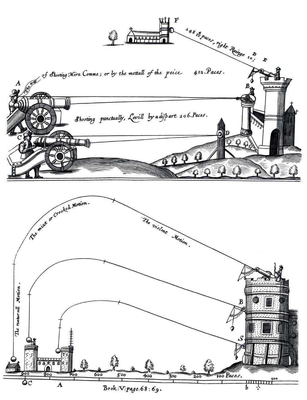
29
Sample pages
Figure A1.52 Trajectories of cannon balls were commonly misunderstood
◆ Thought experiment
An experiment that is carried out in the mind, rather than actually being done, normally because it is otherwise impossible.
Photographs taken in quick succession became useful in analysing many types of motion in the nineteenth century, but the trajectories of very rapidly moving projectiles were difficult to determine until they could be filmed or illuminated by lights flashing very quickly (stroboscopes). The photograph of the bullet from a gun shown in Figure A1.53 required high technology, such as a very high-speed flash and very sensitive image recorders, in order to ‘freeze’ the projectile (bullet) in its rapid motion (more than 500 m s−1).
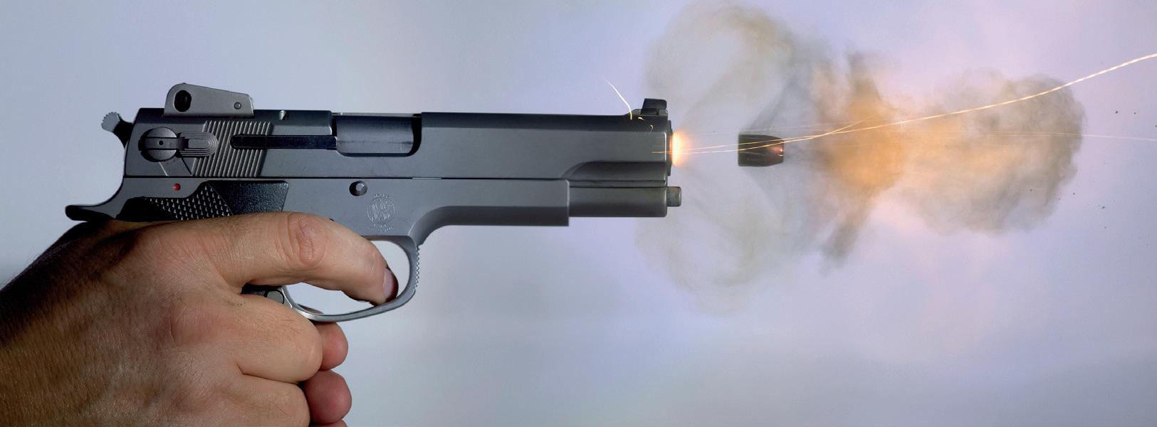
Figure A1.54
Newton’s cannonball thought experiment
‘Newton’s cannonball’ is a famous thought experiment concerning projectiles, in which Newton imagined what would happen to a cannonball fired (projected) horizontally at various very high speeds from the top of a very high mountain (in the absence of air resistance). See Figure A1.54. The balls labelled A and B will follow parabolic paths to the Earth’s surface. B has a greater range than A because it was fired with greater velocity. Cannonball C has exactly the correct velocity that it never falls back to the Earth’s surface and never moves further away from the Earth. (The required velocity would be about 7 k m s−1, but remember that we are assuming that there is no air resistance.) These ideas are developed further in Topic D.1.
Nature of science: Models
In a thought experiment, we use our imagination to answer scientific ‘what if…?’ type questions. Known principles or a possible theory are applied to a precise scenario, and the consequences thought through in detail. Usually, but not always, it would not be possible to actually carry out the experiment.
At the time of ‘Newton’s cannonball’ thought experiment (published in 1728) it would have been impossible to make any object move at 7 k m s−1 and, even if that had been possible, air resistance would have quickly reduced its speed. Nevertheless, the thought processes involved advanced understanding and led to ideas of satellite motion. The first satellite to orbit the Earth was the Russian Sputnik 1 in 1957, which had a maximum speed of about 8 km s−1 and avoided air resistance by being above most of the Earth’s atmosphere.
Another (possible) thought experiment connected to this topic, and involving an assumption of no air resistance, is the dropping of two spheres of different masses from the same height on the Tower of Pisa. See Figure A1.55. Most historians doubt if there was an actual experiment at the Tower of Pisa that confirmed Galileo’s theory that both masses would fall at the same rate.
Figure A1.55 Galileo’s famous experiment to demonstrate acceleration due to gravity
Two further famous thought experiments in physics are Maxwell’s demon and Schrödinger’s cat. Research online to find out how these thought experiments prompted new hypotheses and theories in physics.
Theme A: Space, time and motion
30
Figure A1.53 A bullet ‘frozen’ by high-speed photography
A B C
Sample pages