


This project is supported by the Scottish Government’s Nature Restoration Fund, managed by NatureScot
Work undertaken by

Prepared by: Lorna Cole, Harry Fisher, Jack Zuill, Duncan Robertson, Brayden Youngberg and Mary Sheehan
This report has been prepared exclusively for the use of Glasgow City Region (GCR) Green Network on the basis of information supplied, and no responsibility can be accepted for actions taken by any third party arising from their interpretation of the information contained in this document. No other party may rely on the report and if he does, then he relies upon it at his own risk.
No responsibility is accepted for any interpretation which may be made of the contents on the report.
Contacts: Dr Lorna J Cole
SAC Consulting
Auchincruive Estate
AYR, KA6 5HW
Call: 01292 525 295
Email: Lorna.Cole@sac.co.uk
GCR Green Network
Floor 2, Room 29, 40 John Street
City Chambers East Glasgow G1 1JL
Call: 0141 229 7746 gcrgreennetwork@glasgow.gov.uk
Here we provide a framework to remotely identify species-rich grasslands, map the extent of their networks, and identify opportunity areas where habitat creation could enhance ecological connectivity. To our knowledge this is the first-time that species-rich grassland networks have been identified through a combination of local knowledge, spatial datasets, and biological records to provide a more comprehensive overview of potential networks. In focussing specifically on species-rich grasslands, and including all grassland types (i.e. neutral, calcareous and acid grasslands), the work moves beyond previous network analyses for neutral grassland carried out by the GCRGN.
The approach is adaptable to other regions in Scotland, particularly where high quality spatial data is available. The methodology combines techniques that are highly reproducible to more manual aspects which rely on expert interpretation. Through this methodology we identified 1,826 habitat patches that had a strong potential to be species-rich grasslands in the GCRGN area. Patches tended to exist as small, fragmented habitats with over 67% being less than 2 ha, with larger patches typically constrained to upland locations where pressures associated with agricultural intensification and development are alleviated.
Least-Cost modelling identified species-rich grassland networks for a generic species-rich grassland species. Two dispersal distances were explored to account for mobile species such as bumblebees (i.e. 800 m dispersal) and less mobile species such as solitary bees (i.e. 300 m dispersal). Following this opportunity mapping was conducted to spatially identify areas where creating new grasslands would enhance connectivity.
Network analyses indicated that many species-rich grasslands in the GCRGN area remained isolated for species with low dispersal capabilities highlighting their vulnerability. This was particularly the case in more urban settings where buildings and roads provided barriers to movement. This indicates that there is a need to focus on habitat creation in opportunity areas in built up areas. Networks based on species with higher dispersal powers tended to link up patches to a greater degree and the resultant increased patch size would result in larger, more viable, populations. However, networks were still fragmented indicating that even mobile species would struggle to move freely through the GCRGN area.
The study was primarily limited by the coverage of high-quality spatial datasets, and this was particularly the case in some local authorities. While remote sensing techniques provide comprehensive coverage of the area, the resolution of these datasets is insufficient to identify species-rich grasslands with any level of accuracy. This highlights the importance of detailed on the ground surveying of vegetation (e.g. NVC).
Species-rich grasslands are poorly mapped which makes them particularly vulnerable to development, or alternative land use. Furthermore, with woodlands providing a high-cost habitat for species-rich grassland specialists, policy targets on tree planting could result in the further fragmentation of this important and undervalued habitat. Mapping species-rich grassland networks, and associated opportunity areas will help ensure that the GCRGN can consider them more fully in decision-making.
The loss of semi-natural habitat has been identified as a key driver of insect declines1. With approximately 75% of global crops relying on insects for their pollination services2 , there is growing concern that declines in wild pollinators will adversely impact on food production. Insect pollinated crops are particularly rich in proteins, lipids and micronutrients, and consequently the decline and degradation of pollinator communities has implications to human health and nutrition3 It is, however, not just our crops that depend on these vital pollination services in temperate zones approximately 78% of flowering plants rely on animal-mediated pollination. Healthy pollinating communities therefore underpin the preservation and restoration of semi-natural habitats and in return these habitats provide valuable resources for pollinating insects4 .
A recent expert elicitation process ranked species-rich grasslands as the top habitat for pollinators5 Their value, however, is clearly dependant on management and in the UK the intensification of grassland management practices has resulted in a loss of approximately 97% of species-rich grasslands 6; putting the specialist species they support at risk. In addition to supporting unique communities of plants, invertebrates and birds, species-rich grasslands deliver a wide range of ecosystem services including carbon sequestration and storage, promotion of mental wellbeing, and, if grazed or mown, food production. Species-rich grasslands are truly multifunctional, and their restoration should be a priority to rebuild and enhance Scotland’s natural capital.
Pockets of species-rich grasslands provide steppingstones, allowing species to move around our countryside. The importance of restoring ecological connectivity in our wider countryside is becoming increasingly recognised. Ecological connectivity allows species, and their genetic material, to move more freely through the countryside enabling them to respond to environmental and climate change - resulting in more resilient ecosystems. Furthermore, many
1 Potts, S.G., Imperatriz-Fonseca, V., Ngo, H.T., Aizen, M.A., Biesmeijer, J.C., Breeze, T.D., Dicks, L.V., Garibaldi, L.A., Hill, R., Settele, J. and Vanbergen, A.J., 2016. Safeguarding pollinators and their values to human well-being. Nature, 540(7632), pp.220-229.
2 Klein, A.M., Vaissière, B.E., Cane, J.H., Steffan-Dewenter, I., Cunningham, S.A., Kremen, C. and Tscharntke, T., 2007. Importance of pollinators in changing landscapes for world crops. Proceedings of the royal society B: biological sciences, 274(1608), pp.303-313.
3 Eilers, E.J., Kremen, C., Smith Greenleaf, S., Garber, A.K. and Klein, A.M., 2011. Contribution of pollinatormediated crops to nutrients in the human food supply. PLoS one, 6(6), p.e21363.
4 Ollerton, J., Winfree, R. and Tarrant, S., 2011. How many flowering plants are pollinated by animals?. Oikos, 120(3), pp.321-326.
5 Alejandre, E.M., Scherer, L., Guinée, J.B., Aizen, M.A., Albrecht, M., Balzan, M.V., Bartomeus, I., Bevk, D., Burkle, L.A., Clough, Y. and Cole, L.J., 2023. Characterization factors to assess land use impacts on pollinator abundance in life cycle assessment. Environmental Science & Technology, 57(8), pp.3445-3454.
6 Fuller, R.M., 1987. The changing extent and conservation interest of lowland grasslands in England and Wales: a review of grassland surveys 1930–1984. Biological conservation, 40(4), pp.281-300.
pollinating insects track resources at the landscape scale, moving between habitats to meet their resource requirements through the season7
Butterflies persist in landscapes as metapopulations - populations that exist in discrete habitat patches that are spatially linked through steppingstones that allow movement between patches8. As such, when a population becomes locally extinct, the habitat patch can be recolonised from adjacent patches. The loss of these vital steppingstones can result in the isolation of habitat patches making recolonisation more difficult following local extinction
Restoring ecological connectivity is a key priority to ensure that nature can thrive in the face of environmental change9. Targeting habitat creation to enhance connectivity between habitats through the creation of corridors and steppingstones is fundamental to the Scottish government’s commitment to create a Nature Network across Scotland to enhance ecosystem health, sustainability, and resilience. Through creating a Nature Network and protecting at least 30% of land and seas for nature by 2030 (the 30x30 target) Scotland is committed to meeting to reverse biodiversity loss by 2030 and to restore and regenerate biodiversity by 2045.
Spatially targeting grassland restoration to enhance ecological connectivity is critical to enhance and restore biodiversity and safeguard pollination services. Recognising the value of SRG, and their role in the conservation on biodiversity, the GCRGN commissioned SAC to identify the extent and connectivity of SRG across the networks’ eight local authorities. The identification of SRG networks will help to identify where gaps in connectivity occur enabling the GCRGN to target SRG creation to optimise connectivity. This project is supported by the Scottish Government’s Nature Restoration Fund, managed by NatureScot.
7 Cole, L.J., Brocklehurst, S., Robertson, D., Harrison, W., McCracken, D.I., 2017. Exploring the interactions between resource availability and the utilisation of semi-natural habitats by insect pollinators in an intensive agricultural landscape. Agriculture, Ecosystems & Environment, 246, 157-167.
8 Hanski, I. and Singer, M.C., 2001. Extinction-colonization dynamics and host-plant choice in butterfly metapopulations. The American Naturalist, 158(4), pp.341-353.
9 Lawton, J.H., Brotherton, P.N.M., Brown, V.K., Elphick, C., Fitter, A.H., Forshaw, J., Haddow, R., Hilborne, S., Leafe, R., Mace, G., Southgate, M. 2010. Making space for nature: a review of England’s wildlife sites and ecological network. Department for Food. Agriculture and Rural Affairs, London.
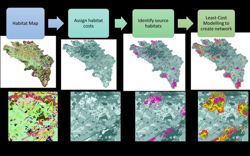
The methodology involves three broad steps. Firstly we identified sites with the potential to be species rich grasslands through a combination of local knowledge, biological records and existing spatial datasets. We then conducted habitat network modelling using a least-cost modelling approach. Networks were conducted for two dispersal distances to reflect mobile species such as bumblebees and less mobile species such as solitary bees. The final state of the process involved opportunity mapping to help identify potential locations where the creation of new patches of species rich grasslands could restore connectivity. An overview of the full process is provided in Figure 1.
Species-rich grasslands (SRG) overall are poorly captured in spatial datasets. To assist in identification of these areas, the Glasgow City Region Green Network (GCRGN) liaised with local authorities to identify known sites. To supplement on the ground knowledge and provide more comprehensive coverage, three main activities were undertaken; specifically, we identified potential areas of SRG via:
• Records of indicator plant species
• Records of indicator butterfly species
• Existing spatial datasets (e.g. Phase 1, HaBMoS, SSSI)
A list of plant species that are potential indicators of SRGs were obtained from the Botanical Society of Britain & Ireland (BSBI) (total 350 species: Annex 1). For these plant species, records from the year 2000 onwards were purchased for the GCRGN area. The accuracy of records varied from 1 m to 1 km. A total of 50,121 records were received.
To help streamline this process, for each 1 km grid square, the indicator plant species richness was calculated (i.e. the total number of indicator plant species recorded within the grid square – data summarised by the BSBI). Each grid square was then categorically assigned to High (>35 BSBI indicator plant species), Medium (11-35 indicator plant species) or Low (<10 indicator plant species recorded) indicator plant richness Squares without records were left blank. This allowed us to map hotspots in botanical richness based on the BSBI records for each 1km grid square (Figure 2). This scale provided a relatively even distribution of squares between the three categories.
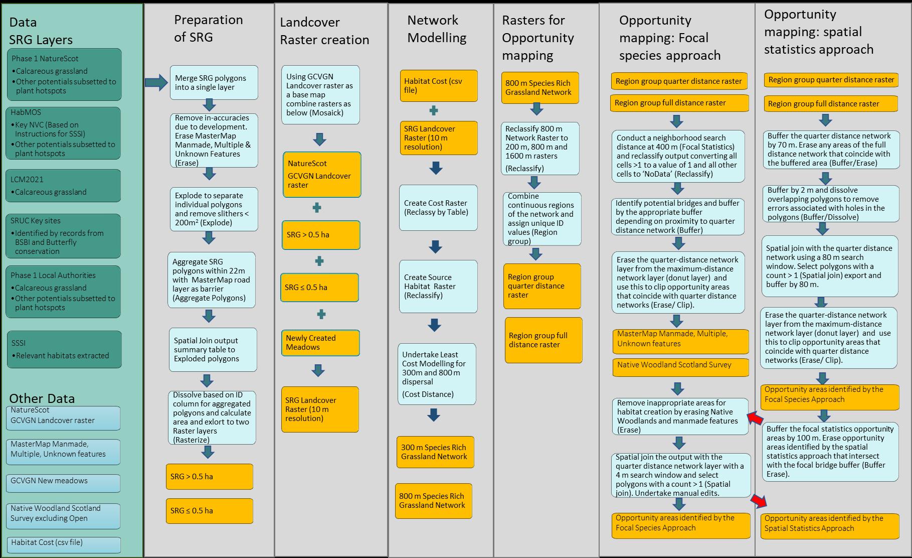
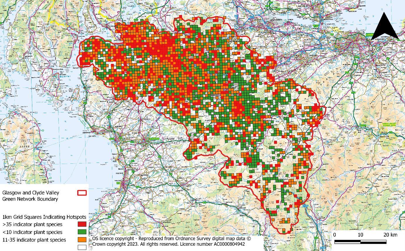
Figure 2: Heatmap showing species rich grassland plant hotspots as identified by BSBI records *Note: Glasgow and Clyde Valley Green Network is now GCR Green Network.
This identified 298 grid squares as plant hotspots (i.e. 1km grid squares with over 35 grassland indicator species). Each square was virtually assessed by an ecologist who assessed if the grid square was likely to contain SRG and if so which habitat parcel had the greatest likelihood. This was achieved by cross referencing aerial footage with BSBI plant records accurate to 100 m resolution or less. BSBI records were buffered by their accuracy to provide a better indication of spatial location of each record.
Ecologists based their decision on the species present alongside aerial images (Figure 3). For example, records accurately pinpointing relatively ubiquitous species (e.g. Cardamine pratensis - Lady's Smock) were ignored, whereas rarer more characteristic species (e.g. Platanthera chlorantha – Greater Butterfly Orchid) or the occurrence of several indicator species (e.g. Achillea millefolium - Yarrow, Hypochaeris radicata – Cat’s Ear, Lathyrus
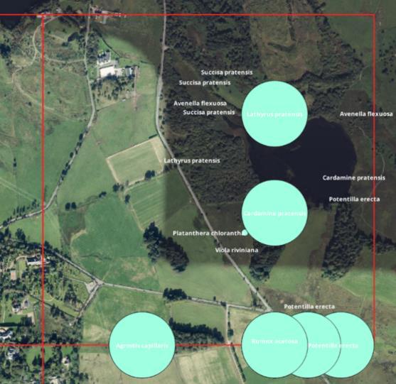
Figure 3: 1 km plant hotspot highlighting species present. The precision of recording is given by the green buffer.

Glasgow City Region: Species Rich Grassland Opportunity Mapping
pratensis – Meadow Vetchling and Rumex acetosa - Common Sorrel) were included. Based on the species present, location and aerial images, each polygon was assigned to acid, neutral, calcareous or wet grassland. This categorisation provided a rough guide to grassland type, however, without ground surveying it was not possible to ensure accuracy.
Habitats patches deemed to have a high likelihood of being SRGs were manually selected from the OS Master Map layer and copied into a new layer. OS Master Map provided a relatively robust means of identifying the spatial extent of the grasslands and allowed for quick transfer of data. The resultant layer consisted of 219 polygons based on plant records, the polygons within this layer were henceforward referred to as SRG.
In addition to plant biological records, butterfly and moth records were also used to identify potential areas of SRG. Following discussion with Butterfly Conservation Scotland, three butterfly species and one moth species were selected as indicators (Table 1). These species were selected as they tend to be restricted to SRG due to caterpillar food plants and they have relatively low dispersal. To align with plant records, lepidopteran records from the year 2000 onwards were obtained from Butterfly Conservation Scotland and inputted to GIS.
Table 1: Butterfly and moth species selected for inclusion
Northern Brown Argus Aricia Artaxerxes Rock-roseHelianthemum nummularium
Small PearlBordered Fritillary Boloria selene Dog-violet - Viola riviniana Marsh Violet - Viola palustris
Grass Rivulet Perizoma albulata Yellow rattle - Rhinanthus minor 531
A total of 1,288 records were obtained and these tended to show spatial clustering. Each cluster of records was systematically viewed in GIS, and the most likely habitat patch based on aerials and plant records were determined
Glasgow City Region: Species Rich Grassland Opportunity Mapping
and extracted from OS MasterMap as SRG (Figure 4). This resulted in 152 polygons derived from lepidopteran records. Again, based on the location and plant species present grasslands were roughly assigned to acid, neutral, calcareous or wet grasslands.
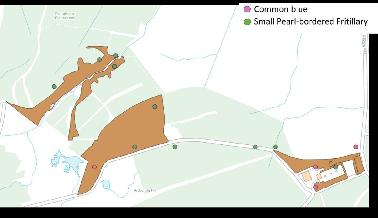
Figure 4: Distribution of butterfly records showing spatial clustering and the selection of habitat polygons based on aerial interpretation.
Spatial Datasets Used For Identification of SRG
To identify SRGs from existing spatial datasets the following datasets were explored:
• NatureScot Phase 1 data10
• NatureScot National Vegetation Classification (NVC) Survey9
• NatureScot Habitat Map of Scotland (HabMoS) 11
o Layer used based on NVC data converted to the EUNIS classification system12
• UKCEH Land Map 202113
• Ordinance Survey MasterMap 202314
• GCRGN: Local Authority Data Phase 115
10 https://cagmap.snh.gov.uk/natural-spaces/category.jsp?code=hs
11 https://opendata.nature.scot/datasets/habitat-map-of-scotland/explore
12 https://www.nature.scot/doc/naturescot-commissioned-report-766-manual-terrestrial-eunis-habitats-scotland
13 https://www.ceh.ac.uk/data/ukceh-land-cover-maps
14 https://www.ordnancesurvey.co.uk/products/os-mastermap-topography-layer
15 Provided directly from GCR Green Network
Glasgow City Region: Species Rich Grassland Opportunity Mapping
• GCRGN: SSSI data14
• GCRGN: Local Authority Data Key Grassland sites14
• GCRGN: Newly Establish Meadows14
The listed datasets contain habitat polygons identified through different methods. Each of these datasets had their strengths and weaknesses when it came to identifying SRG (Table 2) which were dependant on:
• How accurate the survey is with respect to the identification of habitat type and its extent.
• The spatial extent of the dataset with coverage being particularly high for remotely sensed data.
• The age of the data with older datasets being of lower quality due to land use change.
• Detail of classification (e.g. is the data EUNIS level 2 or 4).
Table 2: Strengths and weaknesses of the spatial datasets *Note GCVGN is now GCRGN.
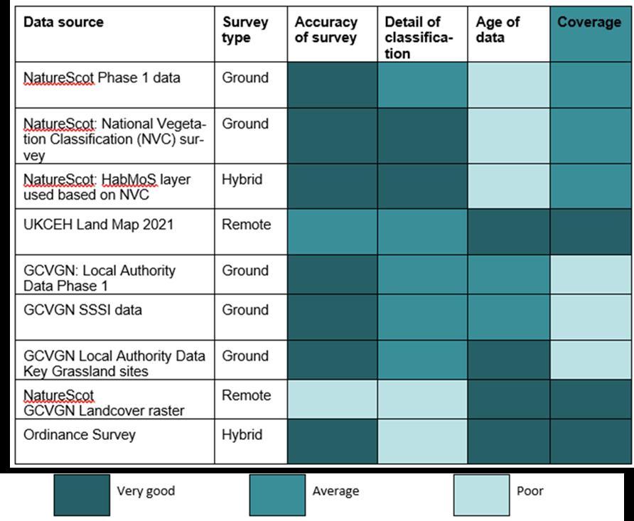
NatureScot’s National Vegetation Classification (NVC) which is derived from detailed plant surveys on the ground provides high accuracy with respect to the
Glasgow City Region: Species Rich Grassland Opportunity Mapping
detail of classification but the data were spatially limited and out of date.
NatureScot’s GCRGN Land Cover Raster, on the other hand, draws from Space Intelligence’s Scotland Habitat and Land Cover Map 2020 which classifies satellite data into habitats using artificial Intelligence. The resultant map provides comprehensive cover, but has inaccuracies due to the limitations of remote sensing, and habitats are only identified to broad habitat type (i.e. EUNIS Level 2) at a 20 m resolution.
As datasets differed in quality, how we utilised and extracted spatial data was dependant on the dataset in question. A description of each dataset and how it was treated is provided in (Table 3). Habitat polygons in spatial dataset were categorised as either:
• SRG Habitat –Habitat polygons with a high likelihood to be SRG selected from datasets with level of accuracy/classification
• Potential SRG Habitats – Habitat polygons with potential to be SRG from the datasets (e.g. Phase 1 unimproved neutral grassland)
• Not SRG - Habitats polygons with a low likelihood of being SRG (e.g. Coniferous woodland plantation).
The HabMoS layer primarily identified habitats at EUNIS level 4. This allowed us to identify SRG based on NatureScot’s Manual of terrestrial EUNIS habitats in Scotland 16 in conjunction with the Guidelines for the Selection of Biological SSSIs17 .
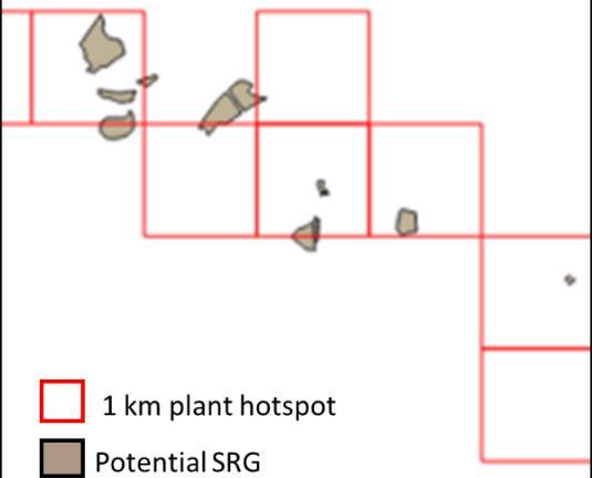
Figure 5: Selection of Potential SRG by 1 km squares identified as Plant Hotspots
The later source uses NVC, so it was first necessary to translate the EUNIS classification to NVC. This was achieved using crosswalk tables that accompanied Nature Scot’s Manual of terrestrial EUNIS habitats.
All polygons identified as Potential SRGs were then cross referenced with Plant Hotspots (i.e. 1 km grid squares with over 35 BSBI indicator plant species). Where Potential SRGs coincided with plant hotspots these were selected and included
16 Strachan, I.M. 2017. Manual of terrestrial EUNIS habitats in Scotland. Version 2. Scottish Natural Heritage Commissioned Report No. 766. SNH Commissioned Report 766: Manual of terrestrial EUNIS habitats in Scotland (nature.scot)
17 Jefferson, R.G., Smith, S.L.N. & MacKintosh, E.J. 2019. Guidelines for the Selection of Biological SSSIs. Part 2: Detailed Guidelines for Habitats and Species Groups. Chapter 3 Lowland Grasslands. Joint Nature Conservation Committee, Peterborough. Chapter 3 Lowland Grasslands (jncc.gov.uk)
Glasgow City Region: Species Rich Grassland Opportunity Mapping
in the final spatial database of SRGs (Figure 5).
Table 3: Overview of each dataset and how data was used. For HabMoS and Phase 1 data further details on the habitat categories selected as SRG or potential SRG are provided in Annex 2
Data & Source Description
NatureScot Phase 1 data
NatureScot: NVC survey
NatureScot: Habitat Map of Scotland (HabMoS)
Phase 1 classification system is relatively broad. These data were used with caution as they were outdated (mainly 19801990s).
Data derived quadrat surveys with plant species classified based on NVC providing detailed habitat information.
Amalgamation of different spatial datasets. Habitats are categorised based on the EUNIS habitat classification system (level 2 to level 5).
UKCEH Land Map 2021 Habitats are classified based on UK Biodiversity Action Plan Broad Habitats.
Ordinance Survey Master Map
GCRGN: Local Authority Data Phase 1
GCRGN designated site data
Natural Features: Broad habitat descriptions for Natural Environment features.
Derived from on the ground Phase 1 surveying for two local authorities (East Dunbartonshire three years and East Renfrewshire 1 year).
Provides an outline of designated sites alongside information on the types of habitats present and their condition.
Use
Calcareous grasslands were selected as SRG. Neutral and Acid grassland were selected as Potential SRG.
Data are nested within HabMoS as a layer converting these data to EUNIS. HabMoS layer used.
Based on the EUNIS classification grassland habitats were either selected as SRG or Potential SRG
Calcareous grassland habitats were extracted as SRG.
Used to sense check habitats, and to provide polygons for selection of SRG based on butterfly and plant records.
Bargenny Hill high quality neutral grassland included as SRG. Other Potential SRG (identified from Phase 1 descriptions) were selected where coinciding with plant hotspots.
From the habitat descriptions, likely habitats were extracted as SRG Habitat. For sites with multiple habitats, aerial footage was used to identify grasslands within the designated site and these polygons were extracted and classified as SRG Habitat.
GCRGN Local Authority Data
Key Grassland sites
GCRGN Newly established meadows
Glasgow City Council and South Lanarkshire provided maps of species-rich grassland sites on paper format and these were digitised by the GCRGN.
East and West Dunbartonshire provided maps of newly established meadows. These were digitised by GCRGN.
Data included as SRG Habitat
To include in habitat map as new meadows with a Cost of 1 (i.e. habitats allowing for free movement)
Glasgow City Region: Species Rich Grassland Opportunity Mapping
In addition to the spatial datasets used to identify SRG, several other spatial datasets were used during the modelling process. These are summarised in Table 4.
Table 4: Overview of spatial datasets used during the modelling process
Data & Source Description
NatureScot GCRGN Landcover raster18
Ordinance Survey Open Roads21
Ordinance Survey MasterMap
Native Woodland Scotland Survey22
Raster that combines Space Intelligence’s Scotland Habitat and Land Cover Map 202019 (re-sampled to 10 m resolution) and Ordnance Survey data urban, road and water features20. Habitat data at EUNIS level 2 and thus insufficient detail to identify SRGs.
This provides detailed mapping of the road network in linear format.
Manmade/Multiple and Unknown features. Data includes houses, gardens, roads, railways, and hard standing surfaces.
Inventory of Native Woodlands inclusive of nearly-native woodlands and Plantations on Ancient Woodland Sites (PAWS)
Use
Data used as baseline habitat map for least-cost habitat network modelling. From this habitat map and the identified SRG habitat a cost raster was derived.
Used as a barrier feature when aggregating polygons. Motorways were buffered by 10 m, A and B roads by 5 m for and smaller roads by 2 m
Used to clean up the SRG database by removing habitat polygons that are no longer SRG. Used to erase opportunity areas that coincide with roads, buildings etc.
Used to erase opportunity areas that coincide with ancient woodland sites. For this habitat parcels relating to Open land habitat (i.e. <20% canopy cover) were not included.
To determine the accuracy of the process two sense checking exercises were conducted prior to network modelling. Firstly, we consulted an ecologist with a sound knowledge of the local area (Dr Scott Shanks) to determine if our methodology had picked up SRG habitats known to them. Except for one site where management had changed recently, and a second site where the identified area was too large, our methodology correctly identified known areas.
18 Provided directly from NatureScot
19 https://spatialdata.gov.scot/geonetwork/srv/api/records/88cea3bd-8679-48d8-8ffb-7d2f1182c175
20 https://www.ordnancesurvey.co.uk/
21 https://www.ordnancesurvey.co.uk/products/os-open-roads
22 https://www.data.gov.uk/dataset/da3f8548-a130-4a0d-8ddd-45019adcf1f3/native-woodland-survey-of-scotlandnwss
Glasgow City Region: Species Rich Grassland Opportunity Mapping
Secondly, we cross referenced spatial datasets with a reduced set of indicator plant records. As the BSBI species list contained species which were not solely indicative of species rich grasslands (e.g. bluebells which are frequently found in woodlands and their edges), BSBI records were restricted to 25 species. Specifically, 30 species identified as SRG indicators by PlantLife (Annex 1), minus five species that were deemed to be too ubiquitous to assist in habitat identification (specifically knapweed, meadow buttercup, oxeye daisy, red clover and ribwort plantain). This resulted in a total of 533 plant records.
Using a spatial join (Join attributes by location) these 533 records were joined to the following habitat layers: Ordinance survey MasterMap Natural Features, CEH Landcover map 2021, HabMoS (NatureScot), Phase 1 (NatureScot) and Phase 1 (GCRGN Data). The data was extracted to MS Excel and for each spatial dataset, the number of key plant records falling in each habitat category was determined using Pivot tables. To determine if any key habitat types had been omitted, the highest counts were explored in greater detail. When exploring the summaries we considered the frequency of different habitat types, and the fact that woodland edges often support SRG indicators. For example, high counts of SRG indicators were found in OS MasterMap agricultural land category –however this is simply due to the extent of this habitat in the GCRGN area. The summary counts are provided in Annex 3. This exercise highlighted that the HabMoS habitat Other Agrostis-Festuca grassland had a relatively high incidence of indicator plant records, and this habitat was therefore included as SRG.
Following initial modelling, a final sense checking exercise involved holding eight workshops engaging the local authorities in the GCRGN area. During these workshops, stakeholders identified 146 areas of SRG not previously identified. Additionally, they also identified areas of SRG that had been lost, or reduced in size, following development. These were incorporated into the manipulated dataset and network modelling and the identification of opportunity areas were repeated.
SRG layers identified through butterfly and plant records and the spatial datasets outlined were combined in QGIS Version 3.28.3-Firenze. To ensure we could trace back the source of individual polygons we first created a column in each attribute table relating to the data source. The layers were then combined. This kept the integrity of each dataset intact (with a column depicting the spatial dataset the data was originally derived from). As data were derived from different sources, there was overlap between SRG polygons identified from different datasets.
Prior to network analyses, several operations were undertaken to tidy up the SRG dataset and which were conducted in ArcGIS Pro Version 3.1.0. Polygons of SRGs derived from different data sources often coincided, resulting in overlapping polygons. As SRG was to be treated as a single habitat, all overlapping polygons (i.e. areas where different spatial datasets had identified the same land parcel as SRGs) were merged into a single polygon using the Merge tool.
It was noted during data extraction that in some instances, sites identified as SRG had been lost to development (e.g. building of houses, roads). From MasterMap a layer of these features was created by selecting Make equal to ManMade, Multiple and Unknown features (hence-force termed MasterMap manmade features). This layer was used to remove all buildings, roads, car parks ect. from the SRG data layer using the Erase tool.
Buglife’s B-Lines modelling makes the assumption that a patch size of 2 ha (i.e. approximately the size of 2.8 football pitches) is the a minimum area to support viable pollinator populations23 . Discussions with the steering group felt that 2 ha was too large to use as a cut off, particularly as SRG patches are fragmented and pollinators survive as metapopulations moving between patches. A habitat patch size of 0.5 ha was therefore selected as a minimum area to be included as Source SRG. To determine the area of individual patches of SRG, we used the Explode tool (single-part-to-multi) to separate each individual habitat patch. Due to the raw datasets and data processing, there were a number of very small fragments of polygons (i.e. slithers) which were removed by deleting all habitat patches with an area of less than 200m2 .
As SRG in close proximity to each other are likely to function as a single habitat patch, we aggregated all polygons that were <22 m apart using the Aggregate Polygons tool following the methodology outlined in Forest Research’s previous work for the Glasgow City Region Green Network. To recognise that roads act as a physical barrier to movement, roads were used as a barrier during aggregation thus ensuring that two SRG patches separated by a road were not aggregated. Using the MasterMap roads layer as a barrier was too process intensive and consequently linear roads were extracted from the Ordinance Survey Open Roads database and buffered by 10 m for motorways, 5 m for A and B roads and 2 m for other roads.
Aggregate Polygons creates a physical join between aggregated habitat patches, thus altering the shape and size of the polygons. Consequently, the
23 Evans, P. 2012. Making B-Lines: A report on the practicalities of developing a B-Lines network, Plan Bee. https://cdn.buglife.org.uk/2020/07/B-Lines-Report-2012_1_.pdf
Glasgow City Region: Species Rich Grassland Opportunity Mapping
accompanying output summary table was joined to the input unaggregated polygon layer using Spatial Join, generating an ID column for aggregated polygons (i.e. two aggregated polygons are given the same ID number). The Dissolve tool was then used to dissolve polygons based on the ID column for aggregated polygons (i.e. using this column as the Dissolve Field), and then the area of the SRG calculated. These steps ensured that habitat patches within 22 m (which were not separated by roads) were treated as single patches and the calculated area reflected the combined area of these patches.
A total of 1,826 species rich grasslands were identified. All SRG ≥ 0.5 ha were assigned as Source SRG (total of 1046) while those < 0.5 ha (total of 780) were assigned as non-Source SRG. These smaller habitat patches were given a Cost Value of 1 which means that while not they are not considered to be source habitat during the network modelling process, it is assumed that species can move freely within the habitat.
In QGIS, the SRG habitat vector layer was separated into two separate layers prior to rasterisation. These were Non-source SRG (i.e. aggregated SRG < 0.5 ha) and Source SRG (i.e. aggregated SRG ≥ 0.5 ha). A third vector layer consisted of ‘newly created meadows’ identified by local authorities was also included (these were also considered as non-source habitat with a Cost Value of 1). Vector layers had an additional column assigning each type of SRG with a unique raster number.
To convert vector layers to rasters, the QGIS tool Rasterize was used. Within this, the vector layers were processed one at a time. The burn in field was selected as the newly made column containing the layers raster value. The fixed value to burn was then selected as this number. The vector layers were rasterised at 10 m georeferenced units (i.e. giving a 10 m resolution). Each rasterisation was done at a high compression. Once the three different vector layers were rasterised at 10 m georeference unit level, they were merged using the Mosaicking tool in QGIS.
The habitat map used in previous habitat network modelling conducted in the GCRGN study area was provided by NatureScot (resolution 10 m). This provided our base map and ensured consistency with previous network modelling analyses undertaken. NatureSot’s GCRGN Land Cover Raster24 was created by combining:
o Space Intelligence’s Scotland Habitat and Land Cover Map 202025
24 Provided directly from NatureScot
25 https://spatialdata.gov.scot/geonetwork/srv/api/records/88cea3bd-8679-48d8-8ffb-7d2f1182c175
Glasgow City Region: Species Rich Grassland Opportunity Mapping
o Ordnance Survey MasterMap Rivers, Roads and Railways26
The final raster was built using the NatureScot Master Map as the base layer, then the SRG layers of < 0.5 ha, then SRG ≥ 0.5 ha, and finally newly created meadows. As such, any SRG identified by our methodology which were actually newly created meadows were classified as newly created meadows rather than SRG Cell size was set to 10 and extent was set to the extent of NatureScot’s MasterMap. Once completed, this produced a raster layer where preassigned raster values for other habitats was set by NatureScot base raster, and Source/Non-Source SRG habitats and newly created meadows were merged on top, replacing whatever previous value had been previously been assigned to that area. This was our final Habitat Raster.
Overview
Habitat Network modelling was undertaken following NatureScot’s Integrated Habitat Network Methodology Handbook27 which was adapted from the BEETLE least-cost habitat network approach developed by Forests Research28 . This approach uses least-cost modelling which recognises that habitats which are not structurally connected (i.e. joined physically), may be functionally connected if the intervening land use allows the focal species to move between habitat patches (Figure 6). Functional connectivity therefore depends on how permeable intervening habitats are and thus recognises that habitats vary in the cost, associated with a species moving through them. This cost encompasses both a physical cost of movement and associated risk. For example, for pollinators coniferous woodlands may be considered high-cost habitats due to costs associated with flying through the dense, shaded habitat.
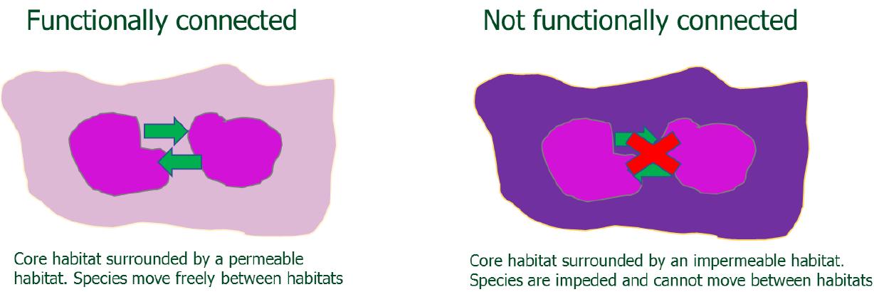
Figure 6: Schematic illustrating functional connectivity
26 https://www.ordnancesurvey.co.uk/
27 Blake, D. & Mattisson, A. 2012. Integrated Habitat Network Methodology Handbook.
28 Watts, K.; Griffiths, M.; Quine, C.P.; Ray, D., Humphrey, J.W. 2005. Towards a woodland habitat network for Wales. Contract Science Report No. 686, Countryside Council for Wales, Bangor, Wales.
Glasgow City Region: Species Rich Grassland Opportunity Mapping
We adopted a focal species approach where the cost of dispersing through different habitat types is represented by the perceived cost for an average SRG species. These costs have been previously identified by NatureScot via expert elicitation. This negates the need for extensive collection of ecological data for different species, and the interpretation of multiple species networks (which can give conflicting information). Adopting this approach ensures resultant outputs are consistent with existing habitat networks created for the Central Scotland Green Network, and for conservation efforts to be directed at a broad generic species rather than simply the species chosen for modelling (Eycott et al. 2007).
All habitats are assigned a cost associated with the focal species moving through the habitat (the cost for source habitats is zero). For example, a cost of one is assigned to habitats that species can freely move through (i.e. Newly Created Meadows and SRG patches that are < 0.5 ha) and a cost of two indicates that the focal species can only travel half of its dispersal distance. The final step involves undertaking least-cost modelling to create the resultant habitat network. Leastcost modelling takes into account the intervening habitats between two areas of source habitat and determines the easiest route between habitat patches29 . Due to the small size of SRG patches, and validity of using edge effects, modelling was conducted without edge effects. An overview of the steps and resultant outputs are provided Figure 7
Network modelling can be conducted for a range of dispersal powers. Here we focussed on two dispersal distances: 800 m (reflecting mobile species such as bumblebees) and 300 m (reflecting less mobile species such as solitary bees).
Habitat Network Modelling was undertaken in ArcGIS Pro using SRUC’s Habitat Networking Tool (Figure 8). The Processing Extent was set to the Habitat Raster and Raster cell size was set to 10 m.
SRUC’s tool requires two input files:
• A Habitat raster created above providing a comprehensive habitat map for the GCR study area including Source SRG (costed as 0), newly created meadows (costed as 1) and SRG patches that were < 0.5 ha (costed as 1).
• A Cost table in csv format which gives an estimated cost for a focal SRG species to move through each habitat included in the Habitat raster (Annex 4).
29 Briers, R., Baarda, P., Heritage, S.N., Bailley, S., Smithers, R., Wilson, J. 2018. Habitat networks–reviewing the evidence base. Scottish Natural Heritage.
Habitat costs were adapted from NatureScot’s costs for a generic semi-natural grassland focal species30 obtained through expert elicitation, taking into account ground truthed data for pollinating insects obtained from south-west Scotland (i.e. butterflies, bumblebees and hoverflies)31 .
The first step of the modelling uses the Reclass by Table tool to reclassify the habitats in the landcover raster using the costs provided in the cost table. This provides a cost raster that translates to the cost of the focal SRG species moving from source habitat (i.e. SRG ≥ 0.5 ha) into the adjacent landscape. This cost raster is then fed into the next step of the model.
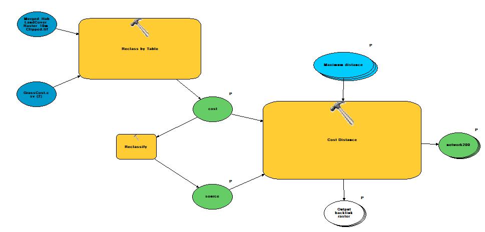
From this cost raster the Reclassify tool is used to create a source habitat raster. This is achieved by reclassifying habitats where the cost is equal to zero (i.e. Source SRG) and setting all other habitats to ‘NoData’.
The final step of the Network Modelling process takes the cost raster (input cost raster) and the source habitat raster (input raster or feature source data) and uses the Cost Distance tool to model distance to the nearest source for each cell in the raster based on the least-accumulative cost over the habitat cost layer. This effectively results in dispersal zones from the source habitat into the surrounding landscape matrix based on the permeability of habitats within the landscape. As such a SRG habitat network is produced. An overview of the modelling process, and outputs are provided in Figure 7 and full model outputs are presented in Annex 5.
30 Blake, D. & Baarda, P. 2018. Developing a habitat connectivity indicator for Scotland. Scottish Natural Heritage Research Report No. 887.
31 Cole, L.J., Brocklehurst, S., Robertson, D., Harrison, W. &d McCracken, D.I., 2017. Exploring the interactions between resource availability and the utilisation of semi-natural habitats by insect pollinators in an intensive agricultural landscape. Agriculture, Ecosystems & Environment, 246, pp.157-167.
Multiple parameters for maximum dispersal distance allow for modelling of species with different dispersal capabilities. As outlined above, we focussed on two dispersal distances 300 m to reflect the distance travelled by less mobile species (e.g. solitary bees) and 800 m to reflect the distance travelled by more mobile species (e.g. bumblebees).
The goal of Opportunity mapping is to identify opportunity areas to target habitat creation that would have a significant impact on reconnecting fragmented SRG habitat networks. Identified areas are split into primary and secondary opportunity areas based on their significance. We follow the methodology developed by Forest Research as part of their work for the Glasgow City Region Green Network and partners and Scottish Natural Heritage looking at conducting a network analysis and opportunity mapping for a range of habitat types. This ensures continuity in the approach to identifying these features across work commissioned by the Partnership.
Due to the fragmented nature of SRGs, and lack of connectivity observed in the 300 m networks, opportunity mapping was based on the 800 m networks. To ensure that species with low dispersal capacity were adequately accounted for, primary opportunity mapping was based on quarter distance networks. This identified opportunity areas for habitat creation features which would connect two or more separate quarter distance network regions (i.e. 200 m dispersal network). Primary opportunity areas therefore create bridges between habitat patches for species with a 200 m dispersal or greater (Figure 9). The secondary opportunity areas consist of habitat creation feature
es that if created would bridge two or more maximum dispersal distance network regions. Thus secondary opportunity areas create bridges between habitat patches for species with a dispersal distance of 800 m (Figure 9). The development of grasslands, or other species-permeable ecosystem, within these opportunity areas (both primary and secondary) would allow for greater connectivity between SRG habitats.
Following Forest Research’s methodology, opportunity areas were identified using two separate methods, a focal statistics method, and a spatial analysis method.
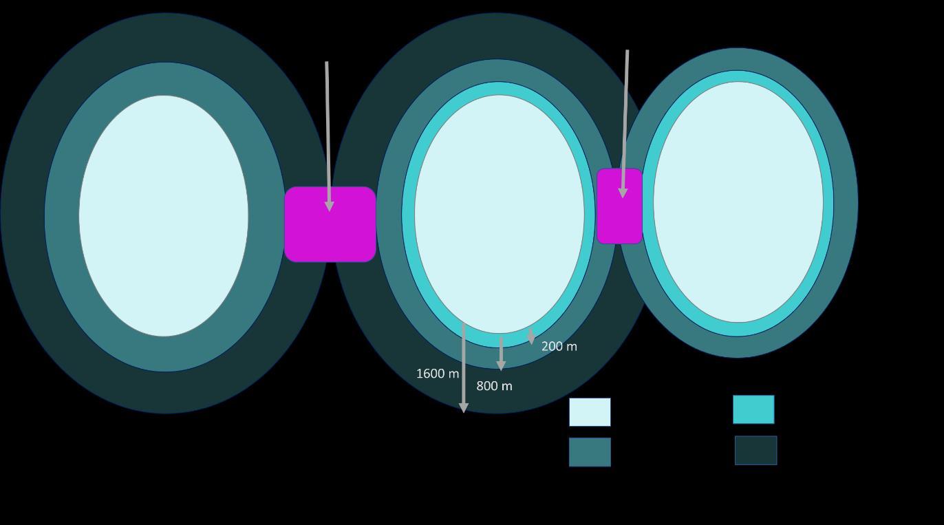
Figure 9: Schematic outlining how primary and secondary opportunity zones create habitat bridges
Preparing Cost Distance Rasters
The Reclassify tool was used to reclassifying the 800m Cost-distance raster created during network modelling into three network rasters required for opportunity mapping. As indicated above these provided quarter distance networks, maximum distance networks and double distance networks. Thus, cells with values <0.25, 1 and 2 times the maximum dispersal distance were reclassified to a value of 1 to give quarter, maximum and double dispersal distance networks respectively. All remaining values were classified at ‘NoData’.
Once reclassified, the Region group tool was used to combine continuous regions of the network cells and assign them unique ID values. The Number of neighbours was set to EIGHT, with all other settings were as default. The results were polygonised and the resulting layer dissolved by their GRIDCODE field using the Dissolve tool
The below method outlines the process for identifying primary opportunity areas and therefore refers to the use of the quarter distance network and maximum distance network. The primary opportunity areas, having been based on the smaller dispersal distance (200 m) to offer the greatest connectivity between these grassland habitats, whereas the secondary areas will require greater species dispersal (800 m) to link habitats together.
The focal statistics approach utilises a raster-based analysis to identify areas of land which lie within a set distance from two or more maximum distance networks.
First a neighbourhood distance region search is conducted using a distance of 400 m (i.e. half the 800 m dispersal distance) using the Focal Statistics tool. The Reclassify tool was used to reclassify the output, converting all cells with a value > 1 to a value of 1 and all other cells to ‘NoData’ . The resulting raster was converted to a polygon – disabling simplify polygons
To identify potential bridges that require a larger buffer, the Select by Location tool was used to select all polygons that are greater than 50 m from the quarterdistance network patches. These polygons were buffered by 200 m using the Buffer tool.
To identify potential bridges that require a smaller buffer, the Select by Location tool was used to select all polygons that lie within 50 m of quarter-distance network patches. The polygons were then buffered by 20 m using the Buffer tool. Using a smaller buffer prevents adjacent bridges from merging which would increase the amount of manual editing required at the final step.
These two buffered layers were then merged into a single layer and the Dissolve tool was used to merge any overlapping polygons The Create multipart features parameter was left unchecked to ensure individual features will be created for each part
The Erase tool was used to create a maximum distance network layer that only contains locations outside of the quarter distance network, i.e. creating a doughnut layer (i.e. erasing the quarter distance network from the maximum distance network). To remove opportunity areas that coincided with quarter distance networks the Clip tool was used to clip the doughnut maximum distance layer from the dissolved opportunity areas
Holes in bridges were then removed by buffering the resultant clipped layer by less than half the raster resolution. We used 2 m as the raster resolution is 10 m. The Dissolve tool was again used to dissolve the resulting layer again ensuring that the Create multipart features parameter was left unchecked. The Spatial Join tool was then used to join the resulting layer with the quarter distance network layer using a search window of 10 m.
It is recognised that some opportunity areas may not be suitable for habitat creation (e.g. buildings, roads, and ancient woodlands). The MasterMap manmade/general and unknown features layer (i.e. representing manmade
GCRGN: Mapping species-rich grassland networks
features such as buildings, gardens, roads and carparks) was used to Erase opportunity areas that overlapped with manmade features using the Erase tool. The Native Woodland Survey of Scotland data was used to create a layer of Native and Nearly Native woodland which included Plantations on Ancient Woodland Sites (PAWS) Land parcels that were open land habitat (i.e. <20% canopy cover) were not included when erasing as it was felt these land parcels provided viable areas for SRG creation The Erase tool as used to remove opportunity areas that overlapped with Native, Nearly Native and PAWS woodlands.
The Buffer tool was used to buffer the resultant layer by 2 m and the Dissolve tool to merge any overlapping polygons (ensuring Create multipart features was disabled). Preform one last spatial join between the latest dataset and the quarter distance network layer with a 4 m search window. To make sure that all opportunities areas connected to more than 1 quarter distance network region (i.e. provide true connections between two distinct networks) all polygons with a join count >1 were selected and exported as a new shape file.
The spatial statistics approach is used as a supplementary approach to identify additional bridges that may not have been identified using the focal statistics method.
The Buffer tool is used to create a 70 m buffer around the quarter distance network. This was found to be a middle ground between not connecting habitats and connecting too many separate network regions. Taking the maximumdistance network (i.e. 800 m network) as the input layer the Erase tool was used to erase any regions of this network that coincided with the 70 m buffer.
In some instances, small holes in polygons could result in single opportunity areas being treated as more than one feature. To prevent this happening, the output file was buffered by a value less than half the raster cell size. In this case 2 m was used. Any overlapping polygons in the output layer were then dissolved into single features using the Dissolve tool. As before, the Create multipart features parameter was left unchecked.
The Spatial join tool was used to join the new layer with the quarter distance network layer using a search distance of 80 m (i.e. a distance larger than the 70 m buffer distance used above). All rows within this new layer with a join count of >1 and an area > 0.01 ha were selected and exported to a new layer (i.e. identifying potential opportunity areas which bridge two quarter distance networks). Buffer this new layer by 80 m.
To remove opportunity areas that coincided with quarter distance networks the Clip tool was used to clip the doughnut layer created in the focal statistic approach from the potential opportunity areas identified by the spatial statistics approach.
To remove opportunity areas already identified by the focal statistics approach, the Buffer tool was used to buffer the final focal statistics opportunity areas by 100 m. The Erase tool was then used to remove opportunity areas identified by the spatial statistics approach that intersect with the buffered focal statistics opportunity areas
As with the Focal Statistics approach, the Erase tool was used to remove any opportunity areas that intersect with MasterMap man-made features and native woodlands (erase layer derived from the Native Woodland Scotland Survey) (see above). Buffer the resultant layer by 2 m and merge any overlapping polygons using the Dissolve tool (again ensure the Create multipart features parameter is left unchecked).
Preform one last spatial join between the latest dataset and the quarter distance network layer (do not use a search distance). To make sure that all opportunity areas are connect to at least two quarter distance network regions (i.e. provide true connections between distinct networks) select all rows that have a join count of >1. The selected polygons provide opportunity areas identified through the Spatial Statistics approach and are exported as a new layer.
Secondary opportunity areas consist of habitat creation features that if created would bridge, two or more maximum dispersal distance network regions (i.e. 800 m). To generate the secondary opportunity areas the process above is repeated by replacing the quarter distance network with the maximum dispersal distance network and the maximum dispersal distance network with the double dispersal distance network.
The final stage of opportunity mapping involved manually editing polygons (i.e. using the Split tool and the Edit Vertices tool) to remove inaccuracies and redundant opportunity areas. This requires a visual assessment of each opportunity area to identify if it makes a true connection between quarter distance networks, and to remove excess opportunity areas created during the modelling which do not contribute to connectivity. To ensure that all opportunity areas are connected to two or more quarter distance networks, a final spatial join was used to confirm that all join counts were > 1.
To identify upland and lowland opportunity areas, Ordinance Survey Terrain 50 (open-source altitude data) was used. For each opportunity area, the Add Surface Information tool in ArcGIS Pro extracted the average altitude using a bilinear interpolation method. Each opportunity area was given an average altitude, and this was used to identify upland (> 200 m) and lowland opportunity areas (≤ 200 m). Opportunity mapping outputs are provided in Annex 6.
Firstly, the primary and secondary opportunity areas were merged into one layer to create a single merged opportunity layer with primary and secondary attributed to each relevant polygon in QGIS. The council area layer was split into eight separate layers, one for each council area, creating eight clip layers. The Clip tool was then used to clip the merged opportunity layer by council area. For each council area, the clipped opportunity areas polygons were exported as a new layer. Where opportunity areas cross council boundaries polygons were split. In some instances, opportunity polygons expanded beyond the GCR area. In these situations, the whole opportunity polygon was included in the council area opportunity layer. This was complete for each council area.
The opportunity layer for each council area was exported as a csv files. For each of the eight council areas, the number and total area of Primary and Secondary Opportunity Areas were calculated using pivot tables in MS Excel (Table 5).
Table 5: Summary information for SRG, Primary and Secondary Opportunity areas for each local authority is provided. The top figure indicates area in hectares and the bottom figure indicates number of SRG patches/opportunity areas. To add context the total council area is also provided, and the number of SRG patches per km2
The cost of meadow creation depends on a variety of factors including location, size of the area, seeds used, presence of weeds/pests, and means of establishment. Plantlife estimates that to create or restore a large meadow will range between £800 to £3,000 per hectare32 (i.e. average £1,900). Lynne Bates (Scottish Wildlife Trust’s Nectar Network coordinator) provided costs of establishment based on green hay versus sowing and additionally gave costs based on three different types of seed options (Table 6).
Table 6: Estimated cost of meadow creation based on different techniques and seeds (Lynne Bates: Scottish Wildlife Trust). Ground preparation for the sown meadow was estimated to cost between £350 - £750 and the midpoint £550 is used in calculations.
It can be seen that costs vary depending on establishment technique. Costs associated with sowing are considerably higher than those associated with green hay. Furthermore, if green hay is obtained from a local location provenance is ensured and plants are adapted to local environmental conditions and pollinator communities. Rough calculations on associated cost of restoring SRG across Opportunity areas are provided in Annex 7.
In comparison to lowland areas, the competition for land in upland environments can be lower due to their lower agricultural productivity and constraints with respect to development. This suggests that it may be more cost effective to restore SRG in upland areas. It can, however, be difficult to access upland areas with machinery, and the ground can be steeply sloped. Establishing SRG in upland areas through mechanical means (e.g. ploughing and sown, scattering of green hay) can therefore be more difficult to achieve.
Adapting grazing management practices could provide a more cost-effective means (e.g. through reduced livestock density or outwintering cattle). This is likely to be easier to achieve in lowland situations due to the large size of upland compartments and the presence of deer. There is the potential to use no fence
32 https://meadows.plantlife.org.uk/making-meadows/how-much-does-it-cost-to-make-a-meadow/
GCRGN: Mapping species-rich grassland networks collars to control livestock grazing with greater accuracy, although these require significant upfront cost. Practitioners are also exploring the use of bale grazing species-rich grass bales during winter to establish more diverse swards. This is a similar approach to green hay, with hay harvested from nearby SRG and the grazing livestock spreading the seed and opening up the sward structure to enable the seed to take hold.
Species-rich grasslands support many specialist species which are threatened by habitat loss and fragmentation. Despite the growing recognition of the importance of these habitats, they remain poorly mapped. Working with the GCRGN and partners we have developed a framework to identify these grasslands remotely through a combination of local knowledge, biological records (plants and butterflies) and open-source spatial datasets. To our knowledge, this is the first time that such data sources have been integrated allowing us to build a more comprehensive picture of the extent of these valuable habitats in the GCRGN area. In focussing solely on species-rich grasslands, and including all grassland types (i.e. neutral, calcareous and acid grasslands), the builds upon previous network analyses for neutral grassland carried out by the GCRGN. Furthermore, in focussing on species-rich grasslands, the work complements existing pollinator network (e.g. B Lines) include a much wider range of habitats as source habitats including scrub and heathland33 34 .
The methodology used is adaptable to other regions in Scotland and will be particularly effective in areas where high quality spatial data is available (i.e. NVC, or EUNIS level 4). The methodology combines techniques that are highly reproducible (i.e. identification of habitat polygons through spatial datasets) to more time consuming manual aspects which rely on expert interpretation of the available data (i.e. the identification of habitat polygons through aerial interpretation and biological records).
Through a combination of biological records and open-source spatial datasets we identified a total of 1,826 habitat patches with a high likelihood of being SRGs. Many of these existed as small, fragmented habitat patches, and 67.5% of these habitats were below 2 ha in size. SRG habitat patches were typically larger in upland areas in comparison to lowland situations which is expected as such areas are less impacted by intensive agricultural practices and development. Indeed during data extraction, it was noted that on several instances habitat patches identified as having a high potential to be SRG had been lost to development. This was also highlighted in the local authority workshops.
To accurately identify SRG high quality spatial data is required. Remotely sensed data, while providing comprehensive coverage of the area, was not available at
33 Paterson, G.B., Smart, G., McKenzie, P. and Cook, S., 2019. Prioritising sites for pollinators in a fragmented coastal nectar habitat network in Western Europe. Landscape ecology, 34, pp.2791-2805.
34 Evans, P. 2012. Making B-Lines: A report on the practicalites of developing a B-Lines Network. Buglife, UK.
GCRGN: Mapping species-rich grassland networks
sufficient resolution to accurately identify SRG (e.g. Space Intelligence’s Scotland Habitat and Land Cover Map 2020 provides classification to EUNIS level 2). Assigning SRG was relatively straightforward when dealing with the HabMoS data layer that classified habitats at EUNIS level 4/5 (derived from NVC data). Phase 1 data, on the other hand, provided some indication – however the level of detail was typically insufficient to conclude that an area of grassland was species-rich. For example, semi-improved neutral grassland would encompass both speciesrich and species-poor sites. This highlights the importance of mapping habitats at a more refined scale which captures vegetation type.
In addition to the simple occurrence and size of SRG habitat patches, the likelihood of detecting SRG will be influenced by a range of factors including the geographical extent of existing spatial datasets, the accessibility and frequency that habitats are visited (influencing biological recording), ease of identifying habitats via aerial footage, and site designations with designated sites having more comprehensive data.
The availability of spatial data varied between local authority areas, with East Renfrewshire having the most comprehensive coverage and North and South Lanarkshire the least (Figure 10). The extent of spatial coverage was reflected in the incidence that SRG was detected with the lowest incidence in North and South Lanarkshire (0.32 and 0.31 patches per 1 km2, respectively (Table 5).
The density of biological records also differed between local authorities with densities higher in Glasgow City than South Lanarkshire (Figure 11). The occurrence of indicator plant species will be dependent on a variety of things in addition to habitat suitability including the area of a specific habitat and where it is located. Locations that are densely populated (e.g. towns and cities), more heavily visited (e.g. popular walks such as the Falls of Clyde), or with greater accessibility (i.e. proximity to footpaths/car parks) tend to have a greater incidence of biological records than more remote, inaccessible areas. Consequently, small patches of SRGs are less likely to be detected in remote locations via biological records.
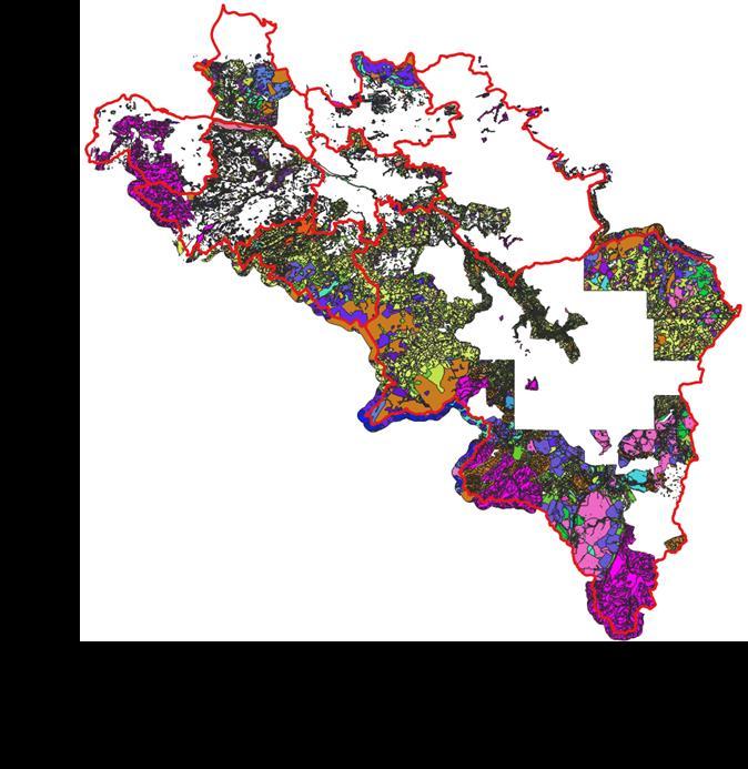
Figure 10: Extent of existing spatial datasets from which SRG were identified

This is particularly interesting given that such locations are likely to be less impacted by human activities and thus have a greater chance of supporting remaining fragments of SRGs.
It was also difficult to accurately determine if a grassland was neutral, acid, calcareous or wet via plant records, and aerial interpretation. While each grassland has characteristic plant species, often these species occur in other grassland types. For example, wild thyme a characteristic species, is often seen in acid grassland where it grows on calcareous ridges. Plant records do not accurately reflect exact community structure of the vegetation and it is difficult to ascertain the dominance and spatial extent of different species. Consequently, the remote identification of grassland types only provides a rough categorisation and verification would require site visits.
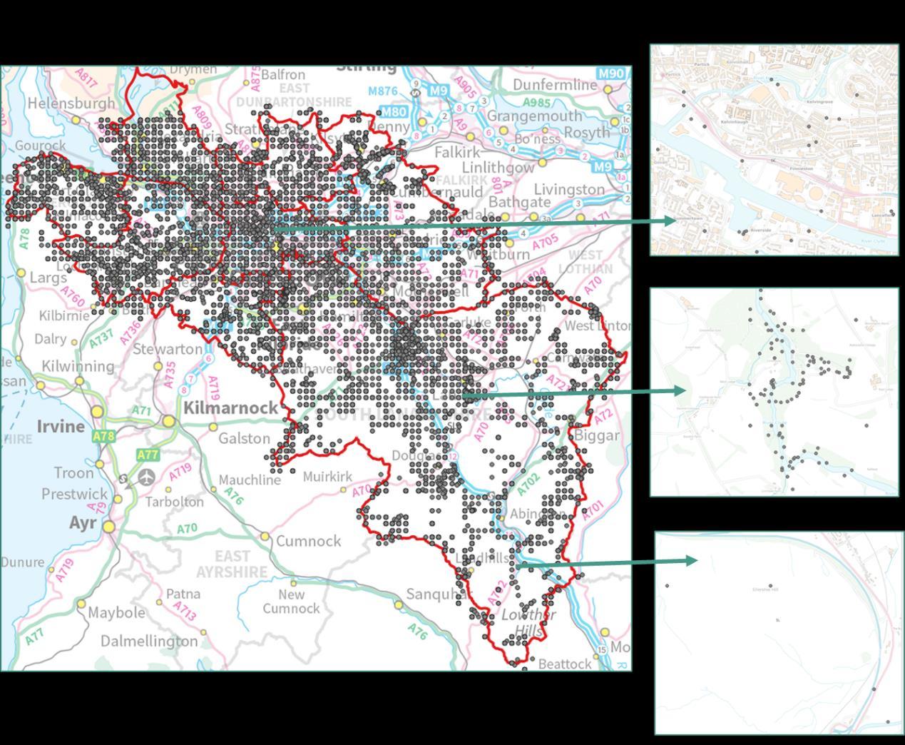
Figure 11: Overview of BSBI records highlighting spatial clustering in more populated, visited areas For consistency close ups are at a scale of 1:10,000
It was found that with a maximum dispersal of 300 m, many patches of source SRG largely remained isolated highlighting the vulnerability of species with low dispersal. This was particularly the case in built up environments where habitats tended to be smaller in size and roads, and surrounding habitats had high costs
GCRGN: Mapping species-rich grassland networks
associated with species movement (Figure 12). This highlights the importance of reconnecting habitat patches in urban areas, and in particular in these areas the need to focus on Primary Opportunity areas that cater for species with low dispersal capabilities.
Our higher maximum dispersal distance of 800 m highlighted a much greater degree of connectivity and on most occasions SRG habitat patches were connected to at least one other habitat patch. While this increased patch size would increase the likelihood of a network patch supporting viable communities of specialist SRG species, there was still significant fragmentation between network patches indicating that even mobile species would struggle to move freely around the area.
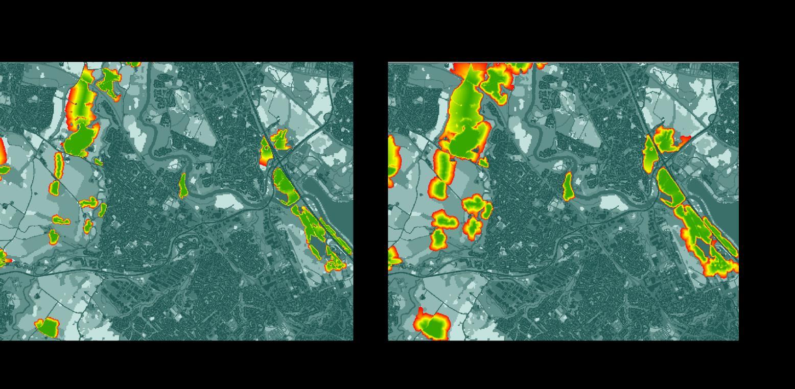
Figure 12: Least-networks illustrating the fragmentation of habitat patch for species with low dispersal capabilities (i.e. 300 m) versus species with higher dispersal abilities (i.e. 800 m)
Networks were more fragmented in some local authorities (e.g. North Lanarkshire) than others (e.g. Inverclyde and East Renfrewshire). However, it is important to take into account that network connectivity is underpinned by the identification of source habitats, which is strongly dependent on the extent of spatial data. With East Renfrewshire having one of the most comprehensive datasets and North Lanarkshire the least.
During this exercise both the aerial interpretation of data and the local authority workshops highlighted that sites identified to potentially be SRG had been lost due to development. While the mapping of SRG networks has its limitations, it does provide an additional source of data to explore when considering development plans. SRG can be difficult to identify, particularly during the winter
GCRGN: Mapping species-rich grassland networks
months, and care should be taken to ensure that networks do not become further fragmented through the loss of key sites. Furthermore, through the identification of opportunity areas the creation or restoration of SRGs can be better targeted to enhance connectivity between habitat patches.
Network and opportunity modelling not only helps to spatially target the creation of new SRG to optimise connectivity, but they could also help to determine where to place other key habitats. In Scotland woodland habitats typically present dense, shaded environments that are relatively costly for SRG species such as pollinating species to move through (i.e. cost is 10). Consequently, woodland creation could result in further fragmentation of SRG within the GCRGN area. The models produced could therefore provide an insight into where woodlands should be placed to reduce adverse impacts on the connectivity of SRGs. Targeting woodland creation is particularly important in light of the Scottish Government’s commitment to expand woodland to 21% of Scotland by 2032 with targets of planting 15,000 hectares per year by 2024 (outlined in their Draft Climate Change Plan35).
It is also important to note that opportunity areas for SRG creation may also provide connectivity for other semi-natural habitats. Consequently, the most appropriate habitat to create will depend on the conservation objectives of an area36 and SRG opportunity maps should be explored alongside opportunity maps for Woodland, Wetland and Bog and Heath produced for the CSGN37 .
The scope of the study was to model SRG networks and consequently the output network is based on the inclusion of all grassland types as source habitat (i.e. acid, neutral, calcareous and wet grasslands). It is, however, recognised that many species are specialist with respect to grassland type. For example, the Northern Brown Argus is largely restricted to calcareous grasslands due to its reliance on rock rose, a calcareous plant species. Within the GCRGN, most grasslands were identified as acid or neutral grasslands, and these were largely segregated spatially with acid grasslands typically occurring at higher altitudes than neutral grasslands. As such, most network patches consist of a single grassland type. To ease interpretation, an indication of grassland type is included in the outputs from the network modelling (Annex 5).
35 https://www.nature.scot/professional-advice/land-and-sea-management/managing-land/forests-andwoodlands/woodland-expansion-across-scotland
36 Humphrey, J., Ray, D., Brown, T., Stone, D., Watts, K. and Anderson, R., 2009. Using focal species modelling to evaluate the impact of land use change on forest and other habitat networks in western oceanic landscapes. Forestry, 82(2), pp.119-134.
37 https://www.nature.scot/doc/central-scotland-green-network-csgn-habitat-connectivity-map-guides
Our modelling selected 0.5 ha as the minimum area to consider source SRG. This is smaller than the area used by Buglife in their B-Lines modelling (2 ha). This minimum area was selected prior to the compiling data, and following discussion with the GCRGN team. It was felt that in more populated areas that SRG frequently persist as small, fragmented habitat patches, which can support metapopulations. Indeed, out of our 1,826 SRG patches, 1046 patches were considered as source SRG (i.e. ≥ 0.5 ha - based on aggregated patch size). If an area of 2 ha had been selected this would only have given 593 source habitats –which would have been largely restricted to upland locations. This would have provided fewer networks across a more restricted geographical area, and would under value the importance of smaller habitat patches that can provide vital steppingstones.
We used a focal species approach to least-cost modelling. This approach uses expert opinion to assign costs associated with moving through specific habitats (i.e. permeability) for a generic SRG species. Habitat costs that are based on expert opinion are clearly subjective38 and expert opinion can vary widely39. To reduce this risk NatureScot uses the Delphi technique to gather expert opinion. This technique allows experts to determine habitat costs independently, they are then given the opportunity to reconsider their cost values based on the values given by other scorers alongside comments.
For our study we drew largely from NatureScot’s costs for a Semi-Natural Grassland species40 , but to strengthen we made modifications based on ground data obtained from the Cessnock Catchment in Ayrshire41. This study explored the density of butterflies, bumblebees and hoverflies in a range of different habitats, and provided a means of ground-truthing expert opinion Largely costs generated by expert opinion were in line with on the ground measures, however, it was felt that values relating to roads (particularly motorways) were too low and these were increased.
There is the potential to support the focal species approach with additional network models that define costs based on the ecology of a few grassland specialist with differing ecology (although for many invertebrate species detailed ecological information is not available). This would allow us to explore networks for species that vary in their vulnerability to fragmentation42. For example, the
38 Humphrey, J., Ray, D., Brown, T., Stone, D., Watts, K. and Anderson, R., 2009. Using focal species modelling to evaluate the impact of land use change on forest and other habitat networks in western oceanic landscapes. Forestry, 82(2), pp.119134.
39 Briers, R., Baarda, P., Heritage, S.N., Bailley, S., Smithers, R. and Wilson, J., 2018. Habitat networks–reviewing the evidence base. Unpublished contract report to Scottish Natural Heritage.
40 Blake, D. & Baarda, P. 2018. Developing a habitat connectivity indicator for Scotland.Scottish Natural Heritage Research Report No. 887.
41 Cole, L.J., Brocklehurst, S., Robertson, D., Harrison, W. &d McCracken, D.I., 2017. Exploring the interactions between resource availability and the utilisation of semi-natural habitats by insect pollinators in an intensive
42 Watts, K., Eycott, A.E., Handley, P., Ray, D., Humphrey, J.W. and Quine, C.P., 2010. Targeting and evaluating biodiversity conservation action within fragmented landscapes: an approach based on generic focal species and least-cost networks. Landscape Ecology, 25, pp.1305-1318.
GCRGN: Mapping species-rich grassland networks
ability of a species to fly would strongly impact on costs associated with crossing watercourses and motorways. Multiple network outputs, with different findings and opportunity areas would be more complex to interpret. We do however try and account for differences in vulnerability through using two dispersal powers to reflect more and less mobile species.
In comparison to other habitats of conservation value such as woodlands and wetlands, SRG are poorly mapped. As a result, they at risk from development and land use change and are less likely to be considered in decision-making. Through combining open-source spatial data with biological records we have developed a framework to identify potential SRG sites. While ground-truthing is required to validate this work, it provides an initial baseline map of SRG in the GCRGN area. SRGs were found to exist in a fragmented state within the GCRGN area, with the majority of habitat patches being less than 2 ha. This is particularly the case in urban areas where development has resulted in habitat fragmentation and buildings and roads provide barriers to dispersal. Through the identification of habitat networks, and opportunity areas for SRG creation the GCRGN are better placed to consider SRG in their decision-making.
Table 7: List of species rich grassland indicator plants: Botanical Society of Britain and Ireland
Achillea millefolium L.
Agrimonia eupatoria L.
Agrimonia procera Wallr.
Agrostis capillaris L.
Agrostis curtisii Kerguélen
Agrostis vinealis Schreb.
Aira praecox L.
Ajuga chamaepitys (L.) Schreb.
Alchemilla acutiloba Opiz
Alchemilla alpina L.
Alchemilla filicaulis Buser
Alchemilla glabra Neygenf.
Alchemilla glaucescens Wallr.
Alchemilla glomerulans Buser
Alchemilla micans Buser
Alchemilla minima Walters
Alchemilla monticola Opiz
Alchemilla subcrenata Buser
Alchemilla wichurae (Buser) Stefánsson
Alchemilla xanthochlora Rothm.
Allium oleraceum L.
Allium scorodoprasum L.
Allium vineale L.
Alopecurus bulbosus Gouan
Anacamptis morio (L.) R.M.Bateman
Anacamptis pyramidalis (L.) Rich.
Antennaria dioica (L.) Gaertn.
Anthriscus caucalis M.Bieb.
Anthyllis vulneraria L.
Aphanes australis Rydb.
Arabis hirsuta (L.) Scop.
Armeria maritima subsp. elongata (Hoffm.) Bonnier
Artemisia campestris L.
Asperula cynanchica L.
Astragalus alpinus L.
Astragalus danicus Retz.
Helictochloa pratensis (L.) Romero Zarco
Avenula pubescens (Huds.) Dumort.
Bartsia alpina L.
Botrychium lunaria (L.) Sw.
Brachypodium pinnatum (L.) P.Beauv. s.s.
Briza media L.
Bromopsis erecta (Huds.) Fourr.
Bromus hordeaceus subsp. ferronii (Mabille) P.M.Sm.
Bromus racemosus L. subsp. racemosus
Bupleurum tenuissimum L.
Campanula glomerata L.
Campanula rotundifolia L.
Cardamine pratensis L.
Carduus tenuiflorus Curtis
Carex binervis Sm.
Carex capillaris L.
Carex caryophyllea Latourr.
Carex divisa Huds.
Carex ericetorum Pollich
Carex filiformis L.
Carex flacca Schreb.
Carex humilis Leyss.
Carex montana L.
Carex muricata L.
Carex ornithopoda Willd.
Carex pilulifera L.
Carex spicata Huds.
Carlina vulgaris L.
Carum carvi L.
Catapodium rigidum (L.) C.E.Hubb.
Centaurea nigra L. s.s.
Centaurea scabiosa L.
Centaurium erythraea Rafn
Cerastium arvense L.
Cerastium fontanum Baumg.
Cerastium pumilum Curtis
Cerastium semidecandrum L.
Ceratocapnos claviculata (L.) Lidén
Chamaemelum nobile (L.) All.
Oxybasis chenopodioides (L.) S.Fuentes
Cirsium acaule (L.) Scop.
Cirsium eriophorum (L.) Scop.
Betonica officinalis L.
Blackstonia perfoliata (L.) Huds.
Clinopodium vulgare L.
Dactylorhiza viridis (L.) R.M.Bateman
Colchicum autumnale L.
Conopodium majus (Gouan) Loret
Convallaria majalis L.
Cotoneaster cambricus J.Fryer & B.Hylmö
Crepis mollis (Jacq.) Asch.
Crepis praemorsa (L.) F.Walther
Cruciata laevipes Opiz
Cynoglossum officinale L.
Cypripedium calceolus L.
Danthonia decumbens (L.) DC.
Daucus carota L.
Avenella flexuosa (L.) Drejer
Dianthus deltoides L.
Draba incana L.
Dryas octopetala L.
Echium vulgare L.
Epipactis helleborine (L.) Crantz
Equisetum ramosissimum Desf.
Euphrasia arctica Lange ex Rostrup
Euphrasia confusa Pugsley
Euphrasia micrantha Rchb.
Euphrasia officinalis agg.
Euphrasia pseudokerneri Pugsley
Festuca filiformis Pourr.
Festuca lemanii Bastard
Festuca longifolia Thuill.
Festuca ovina L.
Filipendula vulgaris Moench
Fragaria vesca L.
Fritillaria meleagris L.
Galium boreale L.
Galium pumilum Murray
Galium saxatile L.
Galium sterneri Ehrend.
Galium verum L.
RGN: Mapping species-rich grassland networks
Cirsium heterophyllum (L.) Hill
Cirsium tuberosum (L.) All.
Gentiana verna L.
Gentianella amarella (L.) Börner
Gentianella amarella subsp. anglica (Pugsley)
Gentianella campestris (L.) Börner
Gentianella germanica (Willd.) Börner
Gentianopsis ciliata (L.) Ma
Geranium columbinum L.
Geranium pratense L.
Geranium sanguineum L.
Geranium sylvaticum L.
Gladiolus illyricus W.D.J.Koch
Gymnadenia conopsea s.l.
Helianthemum apenninum (L.) Mill.
Helianthemum nummularium (L.) Mill.
Helianthemum oelandicum (L.) Dum.Cours.
Heracleum sphondylium L.
Herminium monorchis (L.) R.Br.
Herniaria glabra L.
Himantoglossum hircinum (L.) Spreng.
Hippocrepis comosa L.
Holcus mollis L.
Hordeum marinum Huds.
Hyacinthoides non-scripta (L.) Chouard ex Rothm.
Hypericum hirsutum L.
Hypericum perforatum L.
Hypochaeris glabra L.
Hypochaeris maculata L.
Hypochaeris radicata L.
Iberis amara L.
Inula conyzae (Griess.) Meikle
Jasione montana L.
Juncus compressus Jacq.
Juniperus communis L.
prefTaxonName
Knautia arvensis (L.) Coult.
Koeleria macrantha (Ledeb.) Schult. s.s.
Koeleria vallesiana (Honck.) Gaudin
Gastridium ventricosum (Gouan) Schinz & Thell. Lathyrus aphaca L.
Gaudinia fragilis (L.) P.Beauv.
Genista tinctoria L.
Gentiana pneumonanthe L.
Lathyrus hirsutus L.
Lathyrus linifolius (Reichard) Bässler
Lathyrus nissolia L.
Lathyrus pratensis L.
Leontodon hispidus L.
Leontodon saxatilis Lam.
Lepidium latifolium L.
Leucanthemum vulgare Lam.
Leucojum aestivum L.
Linum bienne Mill.
Linum catharticum L.
Linum perenne L.
Lithospermum officinale L.
Lobelia urens L.
Lotus angustissimus L.
Lotus corniculatus L.
Lotus subbiflorus Lag.
Lotus tenuis Waldst. & Kit. ex Willd.
Luzula campestris (L.) DC.
Luzula multiflora (Ehrh.) Lej.
Luzula spicata (L.) DC.
Lysimachia nummularia L.
Malva moschata L.
Marrubium vulgare L.
Medicago minima (L.) Bartal.
Medicago polymorpha L.
Medicago sativa L.
Melica nutans L.
Mentha pulegium L.
Meum athamanticum Jacq.
Sabulina tenuifolia (L.) Rchb.
Sabulina verna (L.) Rchb.
Moenchia erecta (L.) G.Gaertn.
Muscari neglectum Guss. ex Ten.
Myosotis alpestris F.W.Schmidt
Myosotis discolor Pers.
Myosotis ramosissima Rochel
Nardus stricta L.
Neotinea ustulata (L.) R.M.Bateman
Nepeta cataria L.
Odontites vernus (Bellardi) Dumort.
Oenanthe pimpinelloides L.
Oenanthe silaifolia M.Bieb.
Onobrychis viciifolia Scop.
Polystichum lonchitis (L.) Roth
Potentilla anglica Laichard.
Ononis repens L.
Ononis spinosa L.
Ophioglossum azoricum C.Presl
Ophioglossum lusitanicum L.
Ophioglossum vulgatum L.
Ophrys apifera Huds.
Ophrys fuciflora (Crantz) Moench
Ophrys insectifera L.
Ophrys sphegodes Mill.
Orchis anthropophora (L.) All.
Orchis mascula (L.) L.
Orchis militaris L.
Orchis simia Lam.
Origanum vulgare L.
Ornithopus perpusillus L.
Ornithopus pinnatus (Mill.) Druce
Orobanche elatior Sutton
Phelipanche purpurea (Jacq.) Soják
Orobanche reticulata Wallr.
Oxytropis campestris (L.) DC.
Oxytropis halleri Bunge ex W.D.J.Koch
Bistorta officinalis Delarbre
Bistorta vivipara (L.) Delarbre
Petrorhagia prolifera (L.) P.W.Ball & Heywood
Phleum bertolonii DC.
Phleum phleoides (L.) H.Karst.
Phyteuma orbiculare L.
Picris hieracioides L.
Pilosella officinarum F.W.Schultz & Sch.Bip.
Pilosella peleteriana (Mérat) F.W.Schultz & Sch.Bip.
Pimpinella major (L.) Huds.
Pimpinella saxifraga L.
Plantago coronopus L.
Plantago lanceolata L.
Plantago media L.
Platanthera chlorantha (Custer) Rchb.
Polygala amarella Crantz
Polygala calcarea F.W.Schultz
Polygala serpyllifolia Hosé
Polygala vulgaris L.
Polypogon monspeliensis (L.) Desf.
Scabiosa columbaria L.
Schedonorus pratensis (Huds.) P.Beauv.
Potentilla anserina L.
Potentilla argentea L.
Potentilla crantzii (Crantz) Beck ex Fritsch
Potentilla cryeri Druce ex P.D.Sell
Potentilla erecta (L.) Raeusch.
Potentilla verna L.
Poterium sanguisorba L.
Primula farinosa L.
Primula scotica Hook.
Primula veris L.
Prunella vulgaris L.
Pseudorchis albida (L.) Á.Löve & D.Löve
Puccinellia fasciculata (Torr.) E.P.Bicknell
Puccinellia rupestris (With.) Fernald & Weath.
Pulicaria dysenterica (L.) Bernh.
Pulicaria vulgaris Gaertn.
Pulsatilla vulgaris Mill.
Ranunculus acris L.
Ranunculus bulbosus L.
Ranunculus parviflorus L.
Ranunculus sardous Crantz
Rhinanthus minor L.
Rosa agrestis Savi
Rosa micrantha Borrer ex Sm.
Rosa rubiginosa L.
Rubus saxatilis L.
Rumex acetosa L.
Rumex acetosella L.
Rumex pulcher L.
Sagina saginoides (L.) H.Karst.
Sagina subulata (Sw.) C.Presl
Salvia pratensis L.
Salvia verbenaca L.
Sanguisorba officinalis L.
Saussurea alpina (L.) DC.
Saxifraga aizoides L.
Saxifraga granulata L.
Saxifraga hypnoides L.
Saxifraga oppositifolia L.
Scilla verna Huds.
Scleranthus annuus L.
Scleranthus perennis L.
Scorzonera humilis L.
Scorzoneroides autumnalis (L.) Moench
Selaginella selaginoides (L.) P.Beauv.
Jacobaea erucifolia (L.) G.Gaertn.
Serapias parviflora Parl.
Serratula tinctoria L.
Seseli libanotis (L.) W.D.J.Koch
Sesleria caerulea (L.) Ard.
Sherardia arvensis L.
Silaum silaus (L.) Schinz & Thell.
Silene acaulis (L.) Jacq.
Silene conica L.
Silene otites (L.) Wibel
Silene vulgaris (Moench) Garcke
Spergularia rubra (L.) J.Presl & C.Presl
Spiranthes spiralis (L.) Chevall.
Succisa pratensis Moench
Teesdalia nudicaulis (L.) W.T.Aiton
Tephroseris integrifolia (L.) Holub
Teucrium chamaedrys L.
Teucrium scorodonia L.
Thalictrum alpinum L.
Thesium humifusum DC.
Thymus drucei Ronniger
Thymus pulegioides L.
Thymus serpyllum L.
Tofieldia pusilla (Michx.) Pers.
Torilis nodosa (L.) Gaertn.
Tragopogon pratensis L.
Trifolium arvense L.
Trifolium fragiferum L.
Trifolium glomeratum L.
Trifolium medium L.
Trifolium micranthum Viv.
Trifolium ochroleucon Huds.
Trifolium ornithopodioides L.
Trifolium scabrum L.
Trifolium squamosum L.
Trifolium striatum L.
Trifolium subterraneum L.
Trifolium suffocatum L.
Trinia glauca (L.) Dumort.
Trisetum flavescens (L.) P.Beauv.
Turritis glabra L.
Verbascum lychnitis L.
Veronica chamaedrys L.
Veronica officinalis L.
RGN: Mapping species-rich grassland networks
Veronica spicata L.
Veronica verna L.
Vicia lathyroides L.
Vicia sepium L.
Viola canina L.
Viola hirta L.
Viola lutea Huds.
Viola riviniana Rchb.
Viola rupestris F.W.Schmidt
Viola tricolor L.
Vulpia ciliata Dumort.
Table 8: Plant species indicative of species rich grasslands: Plantlife
Common name
Bulbous buttercup
Common knapweed
Common bird's-foot trefoil
Common rock-rose
Crested dog's-tail
Devil's-bit scabious
Dwarf thistle
Fairy-flax
Field scabious
Glaucous sedge
Greater Butterfly Orchid
Harebell
Lady's bedstraw
Meadow buttercup
Meadow saxifrage
Meadow vetchling
Milkwort sp.
Mountain pansy
Oxeye daisy
Quaking-grass
Red clover
Ribwort plantain
Rough hawkbit
Salad burnet
Self-heal
Red fescue
Spignel
Sweet vernal grass
Thyme
Yellow rattle
Latin Name
Ranunculus bulbosus
Centaurea nigra
Lotus corniculatus
Helianthemum nummularium
Cynosurus cristatus
Succisa pratensis
Cirsium acaule
Linum catharticum
Knautia arvensis
Carex flacca
Platanthera chlorantha
Campanula rotundifolia
Galium verum
Ranunculus acris
Saxifraga granulata
Lathyrus pratensis
Polygala
Viola lutea
Leucanthemum vulgare
Briza media
Trifolium pratense
Plantago lanceolata
Leontodon hispidus
Sanguisorba minor
Prunella vulgaris
Festuca rubra
Meum athamanticum
Anthoxanthum odoratum
Thymus polytrichus
Rhinanthus minor
Table 9 Overview of habitats identified from Phase 1 data (i.e. obtained directly from the GCRGN or from NatureScot’s Open Data Hub) to either include outright, or to subset where they occur in a 1 km grid square identified as plant hotspots.
Code Primary habitat
B1.1 Acid grasslandunimproved
B1.1/A2.2 Acid grasslandunimproved Scrub - scattered
B1.1/A3 Acid grasslandunimproved Parkland/scattered trees
B1.1/A3.1 Acid grasslandunimproved Broadleaved Parkland/scattered trees
B1.1/A3.2 Acid grasslandunimproved Coniferous Parkland/scattered trees
Subset
Subset
Subset
Subset
Subset
B1.1/A3/ A2.2 Acid grasslandunimproved Parkland/scattered trees Scrub - scattered Subset
B1.1/B1.2 Acid grasslandunimproved Acid grassland - semiimproved
Subset
B1.1/B5 Acid grasslandunimproved Marsh/marshy grassland Subset
B1.1/B6 Acid grasslandunimproved Poor semi-improved grassland
Subset
B1.1/C3.1 Acid grasslandunimproved Other tall herb and fernruderal Subset
B1.1/D1.1 Acid grasslandunimproved Dry dwarf shrub heath - acid Subset
B1.1/D5 Acid grasslandunimproved Dry heath/acid grassland Subset
B1.1/E2.1 Acid grasslandunimproved Flush and springacid/neutral flush
B1.1/J1.3 Acid grasslandunimproved Cultivated/disturbed landephemeral/short perennial
Subset
Subset
B1.2/B5 Acid grasslandsemi-improved Marsh/marshy grassland Subset
B1.2/B5/ D2 Acid grasslandsemi-improved Marsh/marshy grassland Wet dwarf shrub heath Subset
B1.2/E3.1 Acid grasslandsemi-improved Fen - valley mire Subset
B2 Neutral grassland Subset
B2.1 Neutral grassland - unimproved Subset
B2.1/A2.2 Neutral grassland - unimproved
B2.1/A2.2 /A3
B2.1/A2.2 /A3.1
B2.1/A2.2 /B5
B2.1/A2.2 /D5
B2.1/A2.2 /I2.2
B2.1/A2.2 /J1.3
B2.1/A3
Neutral grassland - unimproved
Neutral grassland - unimproved
Neutral grassland - unimproved
Neutral grassland - unimproved
Neutral grassland - unimproved
Neutral grassland - unimproved
Neutral grassland - unimproved
B2.1/A3.1 Neutral grassland - unimproved
B2.1/A3.1 /A2.1 Neutral grassland - unimproved
B2.1/A3.1 /A2.2 Neutral grassland - unimproved
B2.1/A3.1 /B5 Neutral grassland - unimproved
B2.1/A3.1 /D5 Neutral grassland - unimproved
Scrub - scattered Subset
Scrub - scattered
Scrub - scattered
Scrub - scattered
Scrub - scattered
Parkland/scattered trees Subset
Broadleaved Parkland/scattered trees Subset
Marsh/marshy grassland Subset
Dry heath/acid grassland Subset
Scrub - scattered Spoil Subset
Scrub - scattered
Cultivated/disturbed landephemeral/short perennial Subset
Parkland/scattered trees Subset
Broadleaved Parkland/scattered trees Subset
Broadleaved Parkland/scattered trees
Broadleaved Parkland/scattered trees
Broadleaved Parkland/scattered trees
Scrubdense/continuous Subset
Scrub - scattered Subset
Marsh/marshy grassland Subset
Broadleaved Parkland/scattered trees Dry heath/acid grassland Subset
B2.1/B2 Neutral grassland - unimproved Neutral grassland Subset
B2.1/B4 Neutral grassland - unimproved Improved grassland Subset
B2.1/B6 Neutral grassland - unimproved Poor semi-improved grassland Subset
B2.1/E3/ A2.2 Neutral grassland - unimproved Fen
Scrub - scattered Subset
B2.1/I2.2 Neutral grassland - unimproved Spoil Subset
B2.1/I2.2/ A2.2 Neutral grassland - unimproved Spoil
Scrub - scattered Subset
B2.2 Neutral grassland - semi-improved Subset
B2.2/A2.2 Neutral grassland - semi-improved
Scrub - scattered Subset
B2.2/A2.2 /A1.1.1 Neutral grassland - semi-improved Scrub - scattered
Broadleaved woodland - seminatural Subset
B2.2/A2.2 /A3.1 Neutral grassland - semi-improved
Scrub - scattered
Broadleaved Parkland/scattered trees Subset
B2.2/A3 Neutral grassland - semi-improved Parkland/scattered trees Subset
B2.2/A3.1 Neutral grassland - semi-improved
Broadleaved Parkland/scattered trees
Subset
B2.2/B5 Neutral grassland - semi-improved Marsh/marshy grassland Subset
B2.2/D5 Neutral grassland - semi-improved Dry heath/acid grassland Subset
B2/A2.2 Neutral grassland - semi-improved Scrub - scattered Subset
B3 Calcareous grassland Include
B3.1 Calcareous grasslandunimproved Include
B3.1/J4 Calcareous grasslandunimproved Bare ground Include
B3.2 Calcareous grassland - semiimproved Include
B5 Marsh/marshy grassland Subset
B5/A2.2 Marsh/marshy grassland Scrub - scattered Subset
B5/A3.1 Marsh/marshy grassland
Broadleaved Parkland/scattered trees Subset
B5/B1.2 Marsh/marshy grassland Acid grassland - semiimproved Subset
B5/B2.1 Marsh/marshy grassland Neutral grasslandunimproved Subset
B5/B6 Marsh/marshy grassland Poor semi-improved grassland Subset
B5/C3.1 Marsh/marshy grassland Other tall herb and fernruderal Subset
B5/D5 Marsh/marshy grassland Dry heath/acid grassland
Table 10 Overview of habitats identified from the Habitat Map of Scotland to either include outright, or to subset where they occur in a 1 km grid square identified as plant hotspots.
EUNIS Code Habitat description
E1.26 H6210 - Semi-natural dry grasslands
E1.7 Closed non-Mediterranean dry acid and neutral grassland Subset
E1.72 [Agrostis] - [Festuca] grassland Yes
E1.72# H6230 - Species-rich Nardus grassland
E1.72x Other Agrostis-Festuca grassland
E1.92 Perennial open siliceous grassland
E1.B1 H6130 - Calminarian grasslands Yes
E2.112 Atlantic Cynosurus-Centaurea pastures Yes
E2.21 Atlantic hay meadows
E2.24 Boreal and sub-boreal meadows Yes
E3.41 Atlantic and sub-Atlantic humid meadows
E3.42 [Juncus acutiflorus] meadows
E3.511 H6410 - Molinia meadows
E3.512 Acidocline purple moorgrass meadows
E3.52 Heath [Juncus] meadows and humid [Nardus stricta] swards
E4.32€ H6150 - Siliceous alpine and boreal grasslands Yes
F4.13 [Molinia caerulea] wet heaths
Table 11: Cross referencing indicator plant species with the Habitat Map of Scotland to provide a count of the number of times each indicator occurred in habitat polygons
G1.A11
D1.2
G1.81
Table 12: Cross referencing indicator plant species with Ordinance Survey MasterMap Natural Features to provide a count of the number times indicator species occurred in each
Table 13: Cross referencing indicator plant species with Phase 1 data obtained from NatureScot to provide a count of the number of times each indicator occurred in habitat polygons
Phase 1 code
A2.1 & A1.1.1
Table 14: Cross referencing indicator plant species with Phase 1 data obtained from GCRGN to provide a count of the number of times each indicator occurred in habitat polygons
Table 15 Cross referencing indicator plant species with CEH’s LCM2021 to provide a count of the number times indicator species occurred in each habitat polygon
Table 16: Cost values for each EUNIS habitat in the final Habitat Raster.
J4.2.4

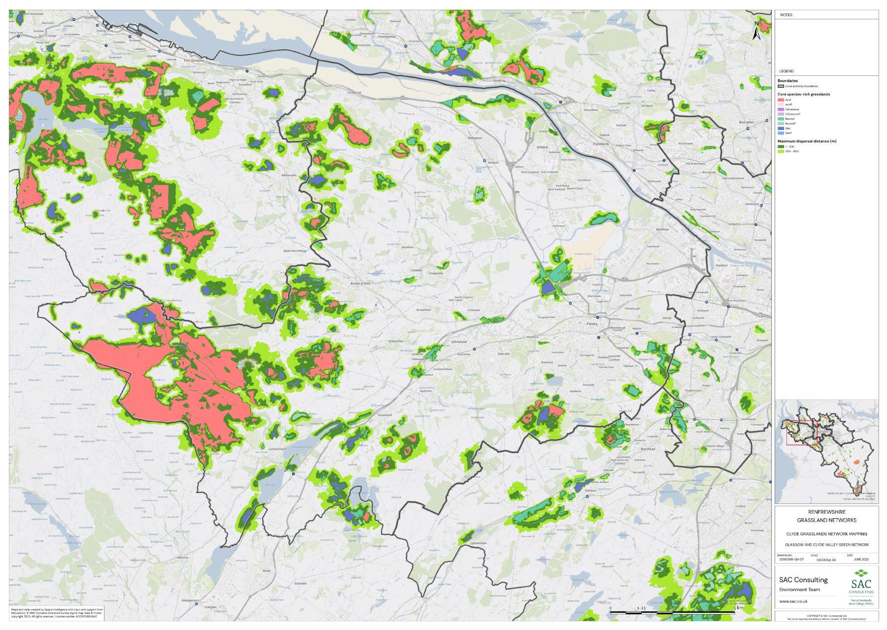
GCRGN: Mapping species-rich grassland networks
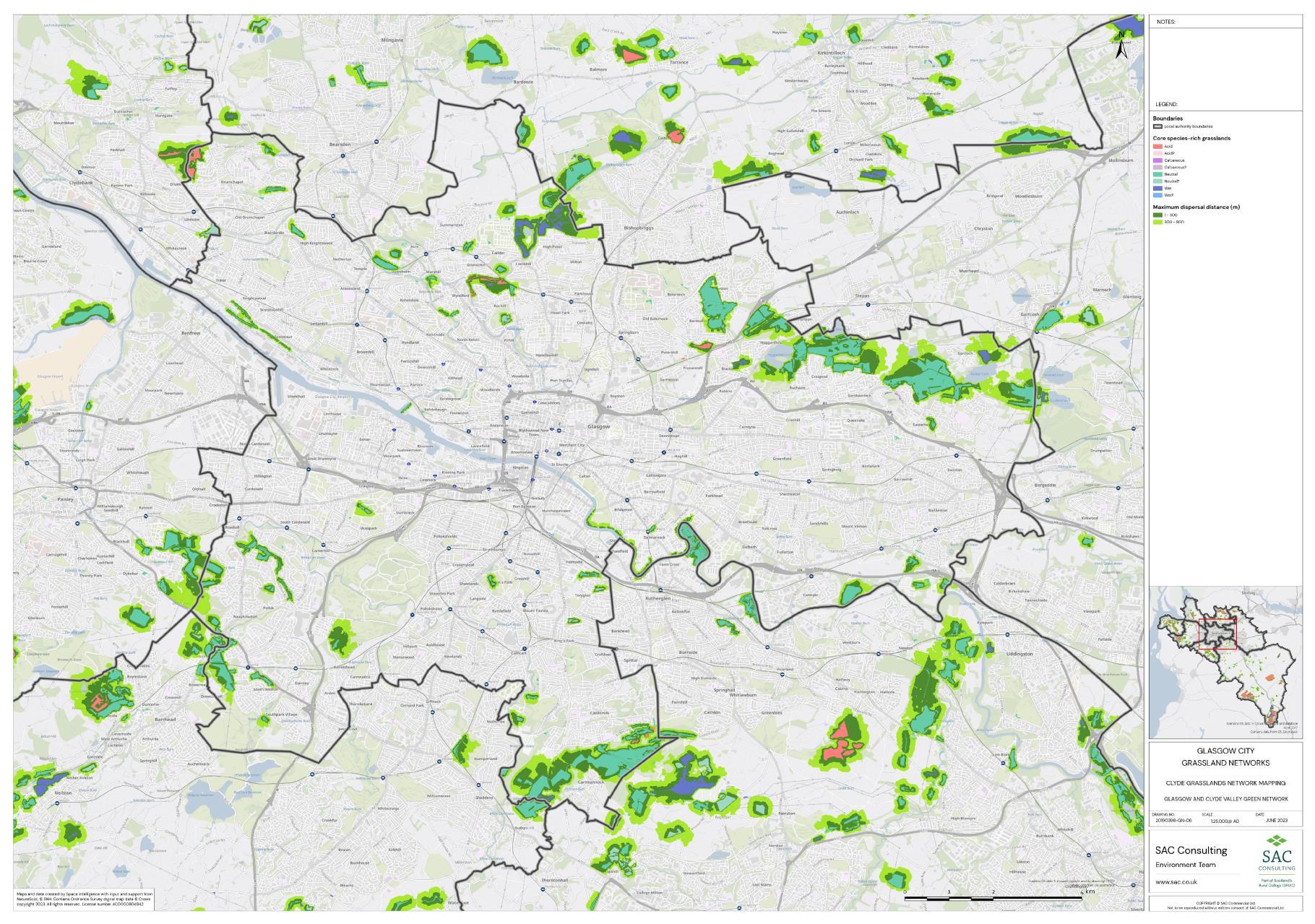
GCRGN: Mapping species-rich grassland networks
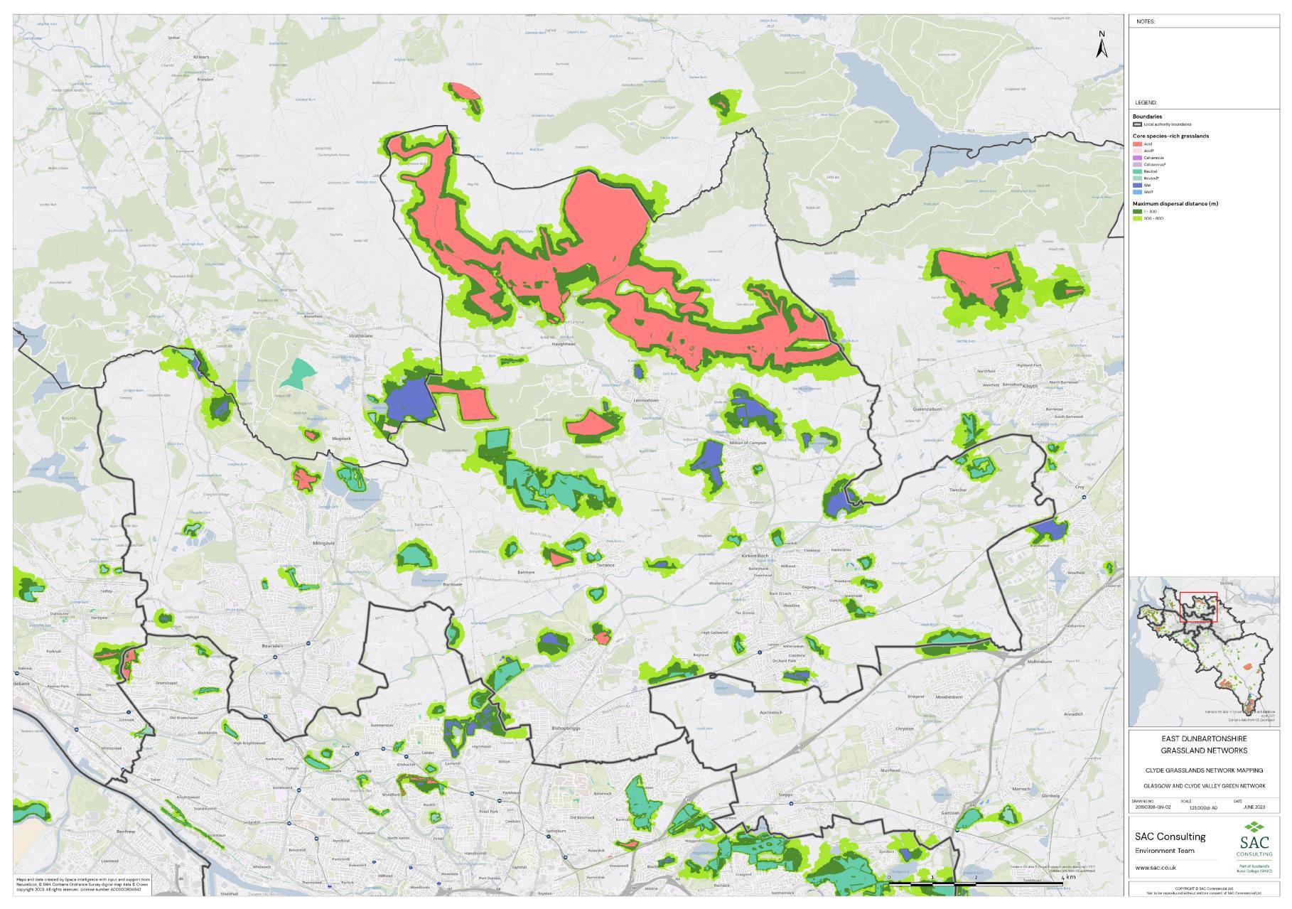
GCRGN: Mapping species-rich grassland networks
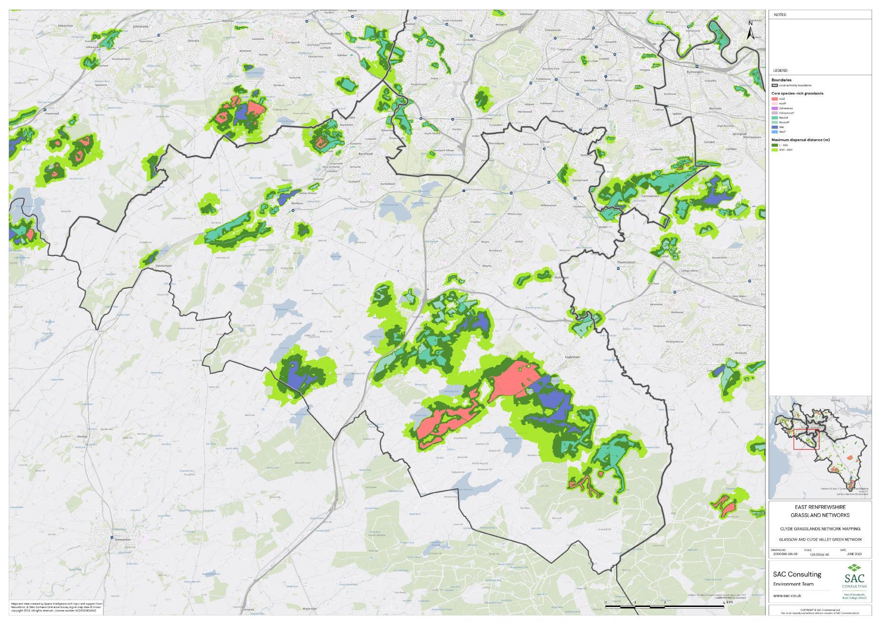
GCRGN: Mapping species-rich grassland networks
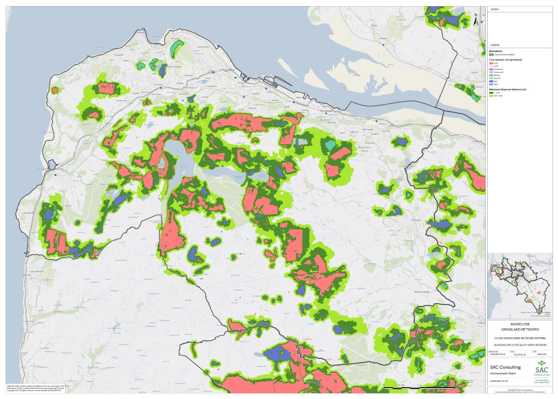
GCRGN: Mapping species-rich grassland networks
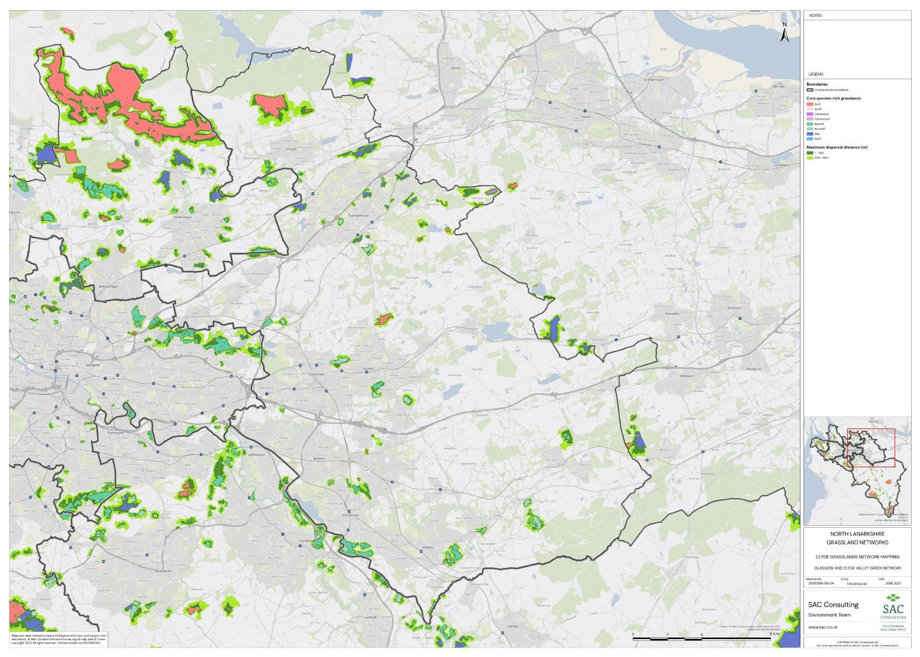
GCRGN: Mapping species-rich grassland networks
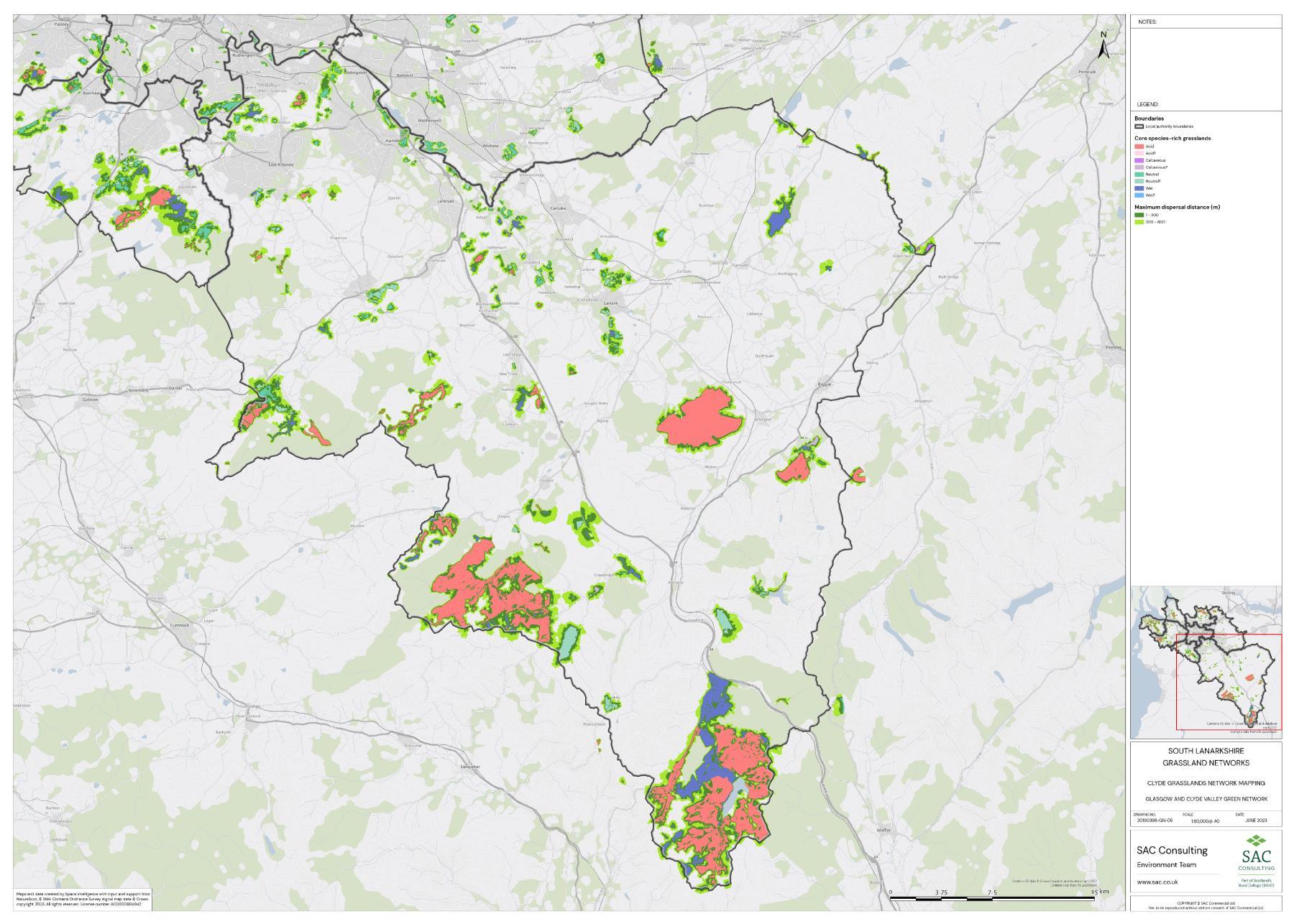
GCRGN: Mapping species-rich grassland networks
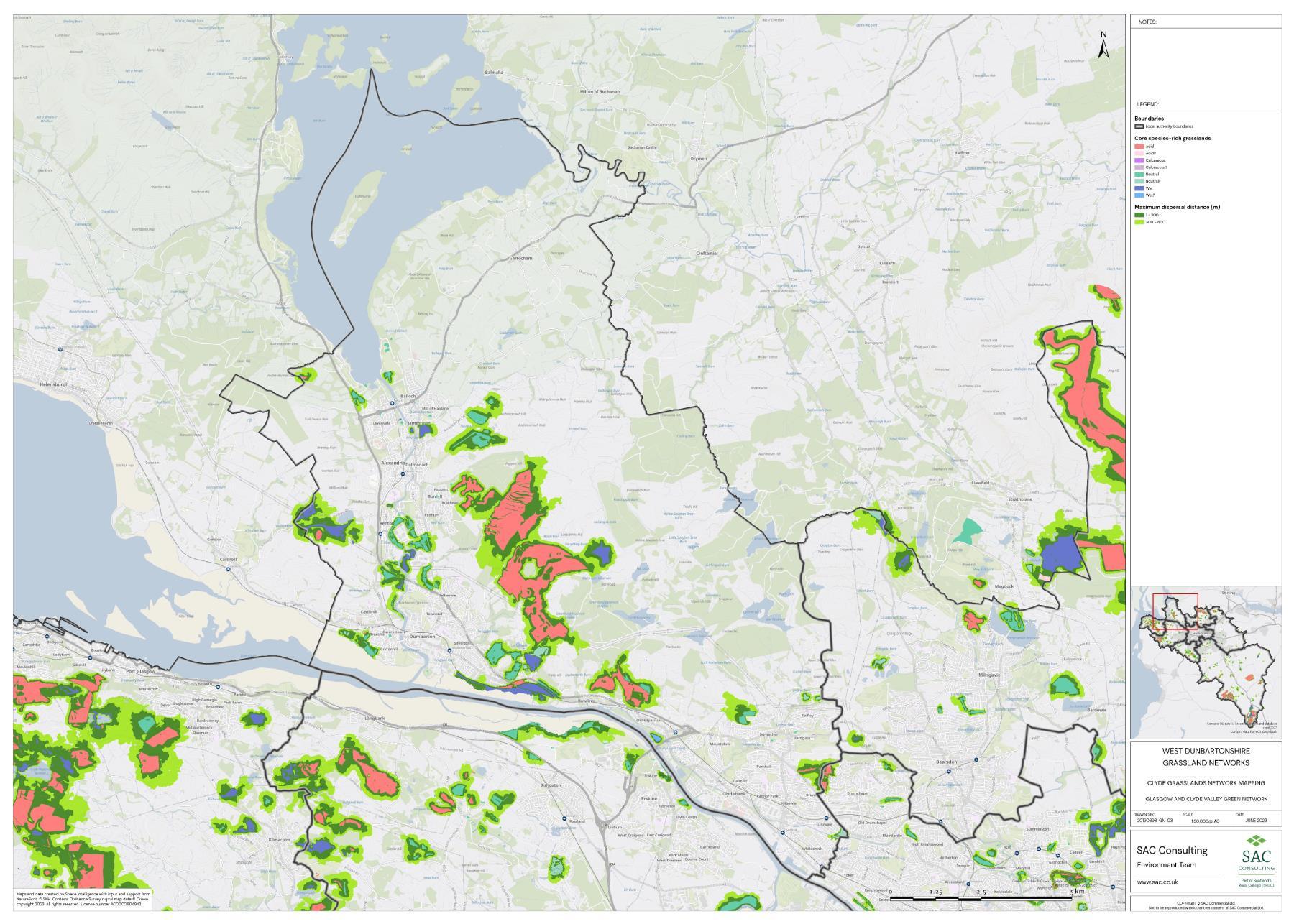
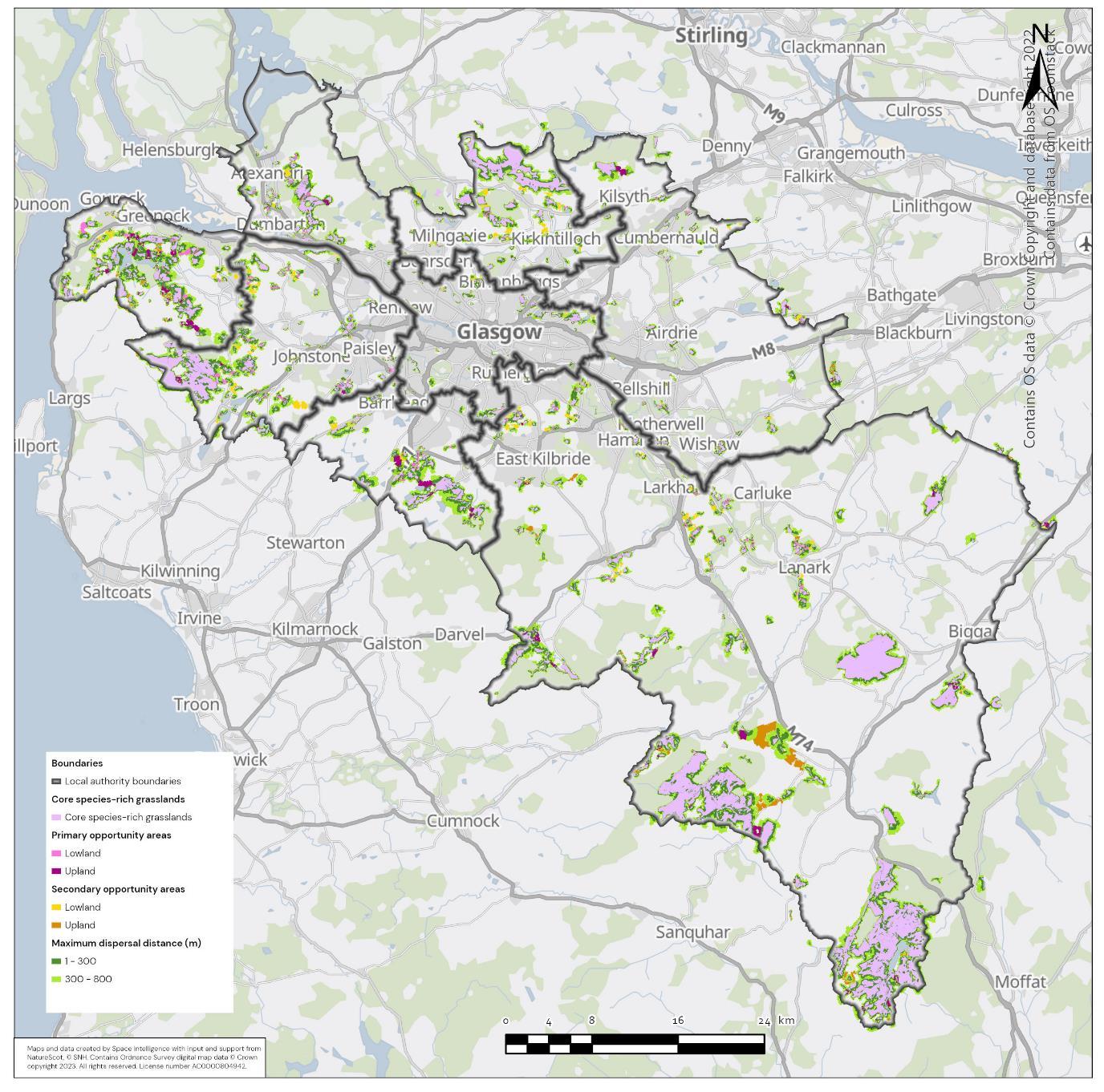
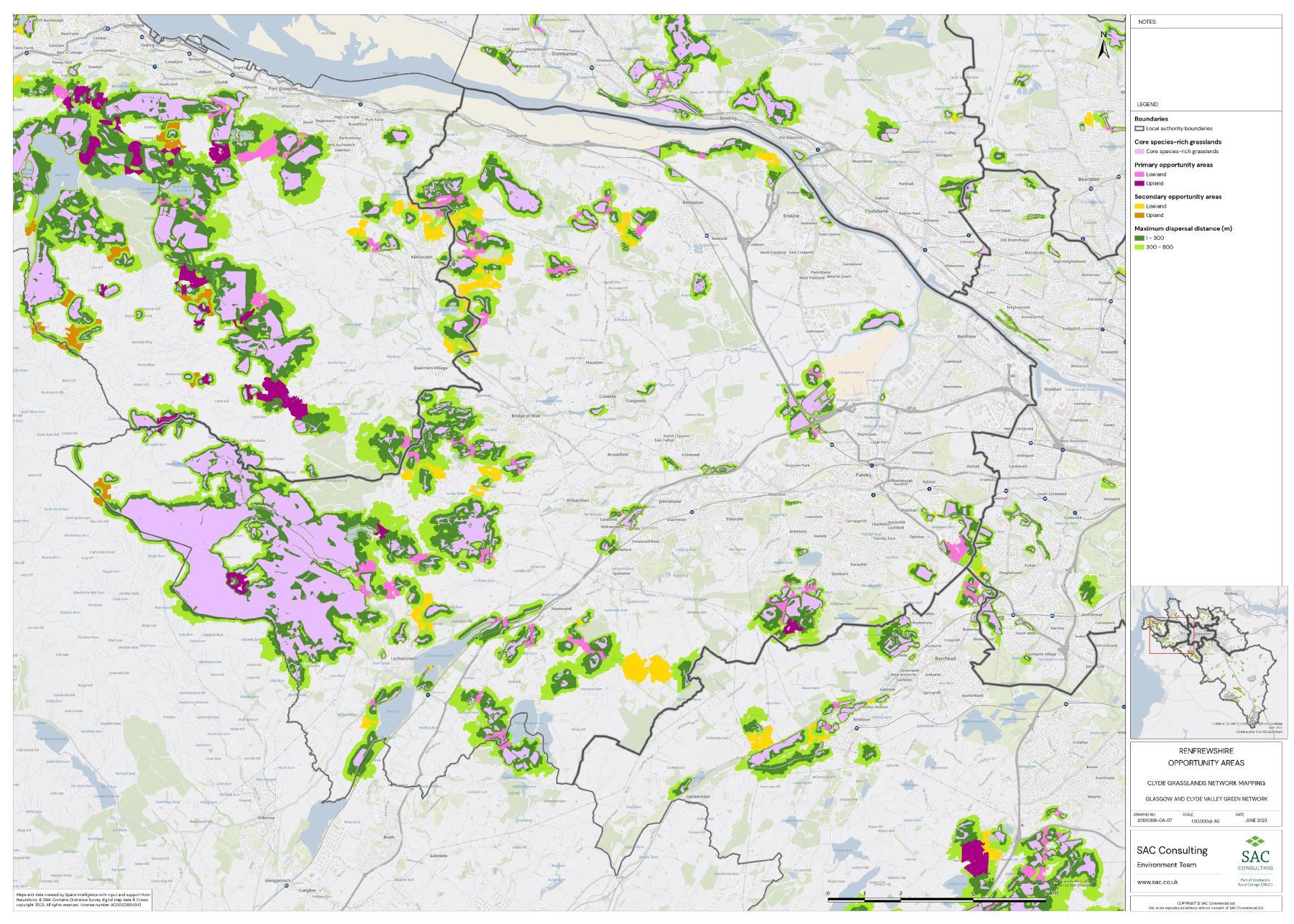
GCRGN: Mapping species-rich grassland networks

GCRGN: Mapping species-rich grassland networks
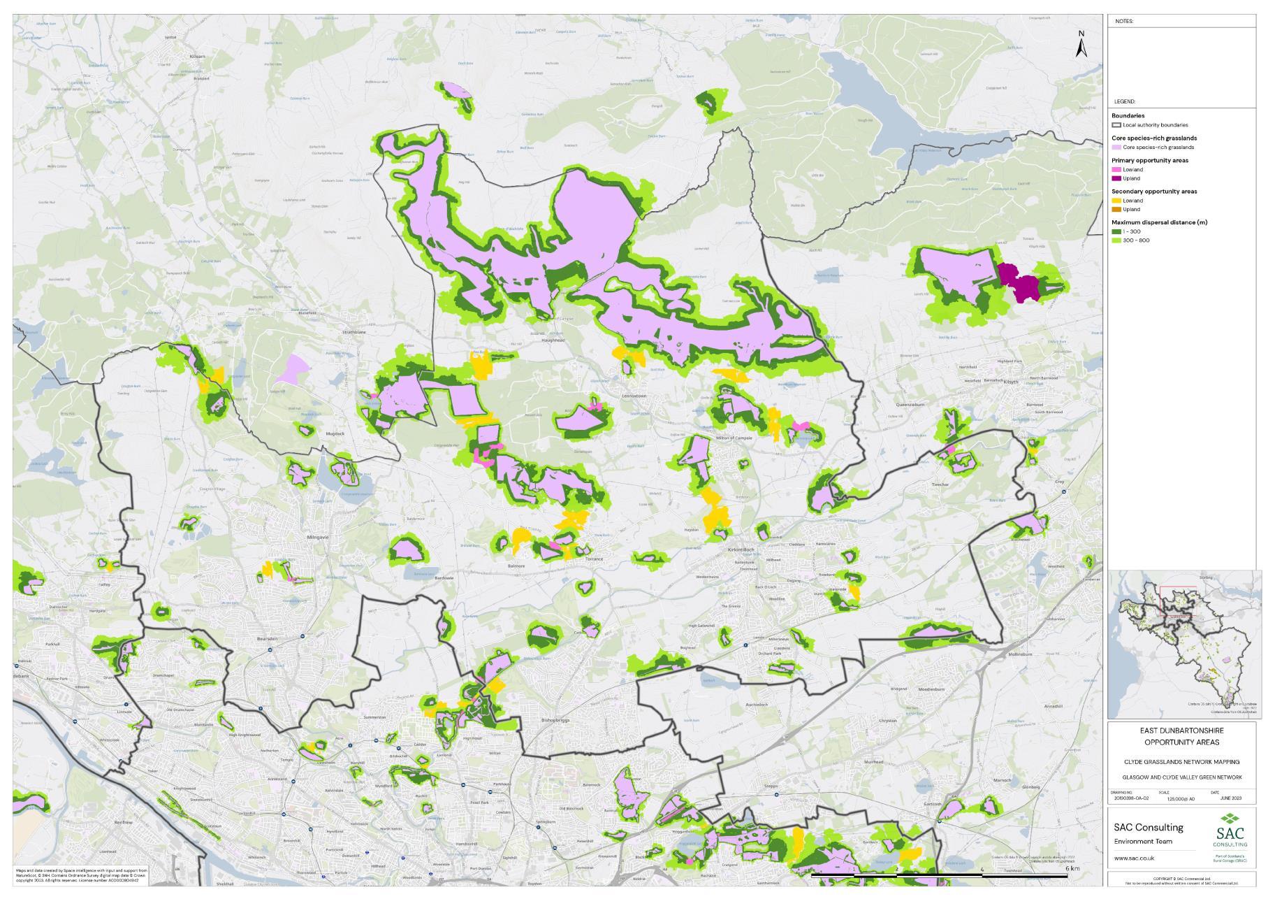
GCRGN: Mapping species-rich grassland networks
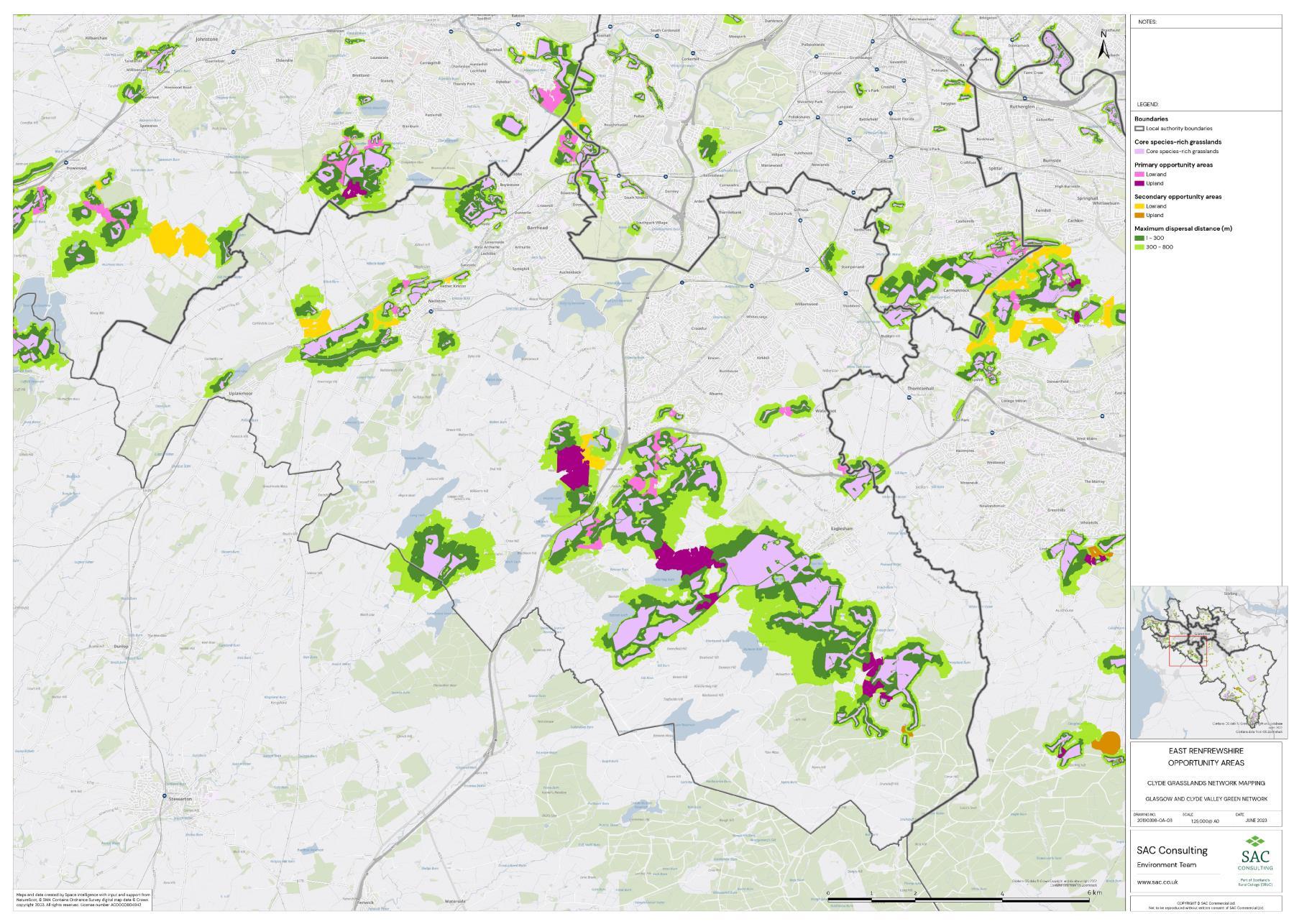
GCRGN: Mapping species-rich grassland networks
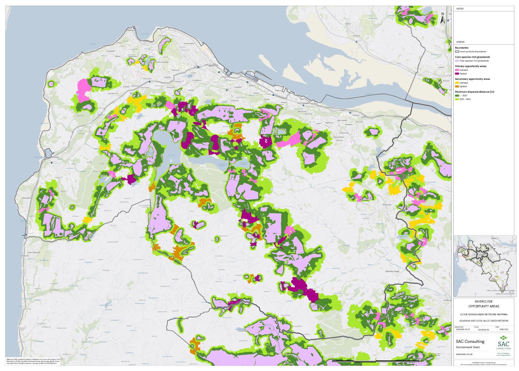
GCRGN: Mapping species-rich grassland networks
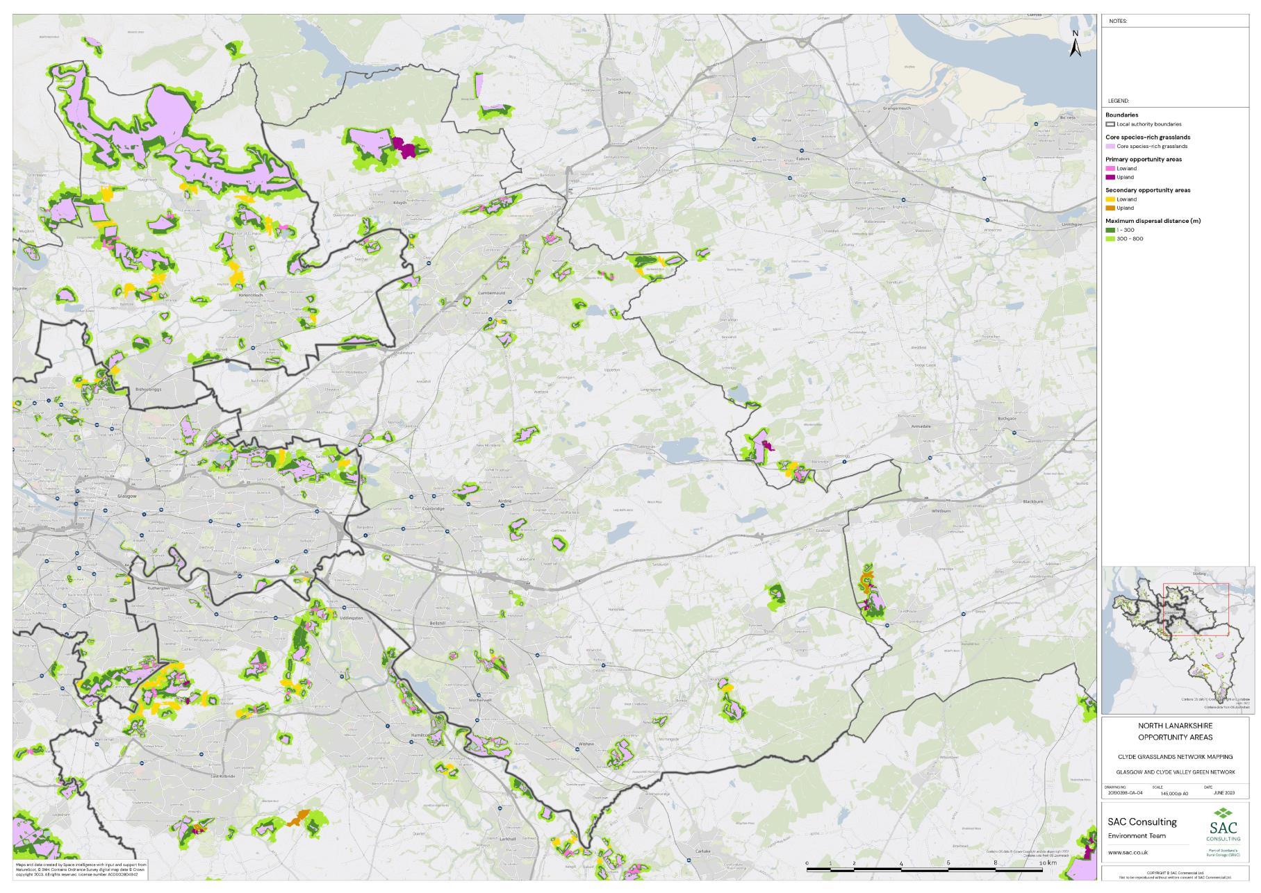
GCRGN: Mapping species-rich grassland networks
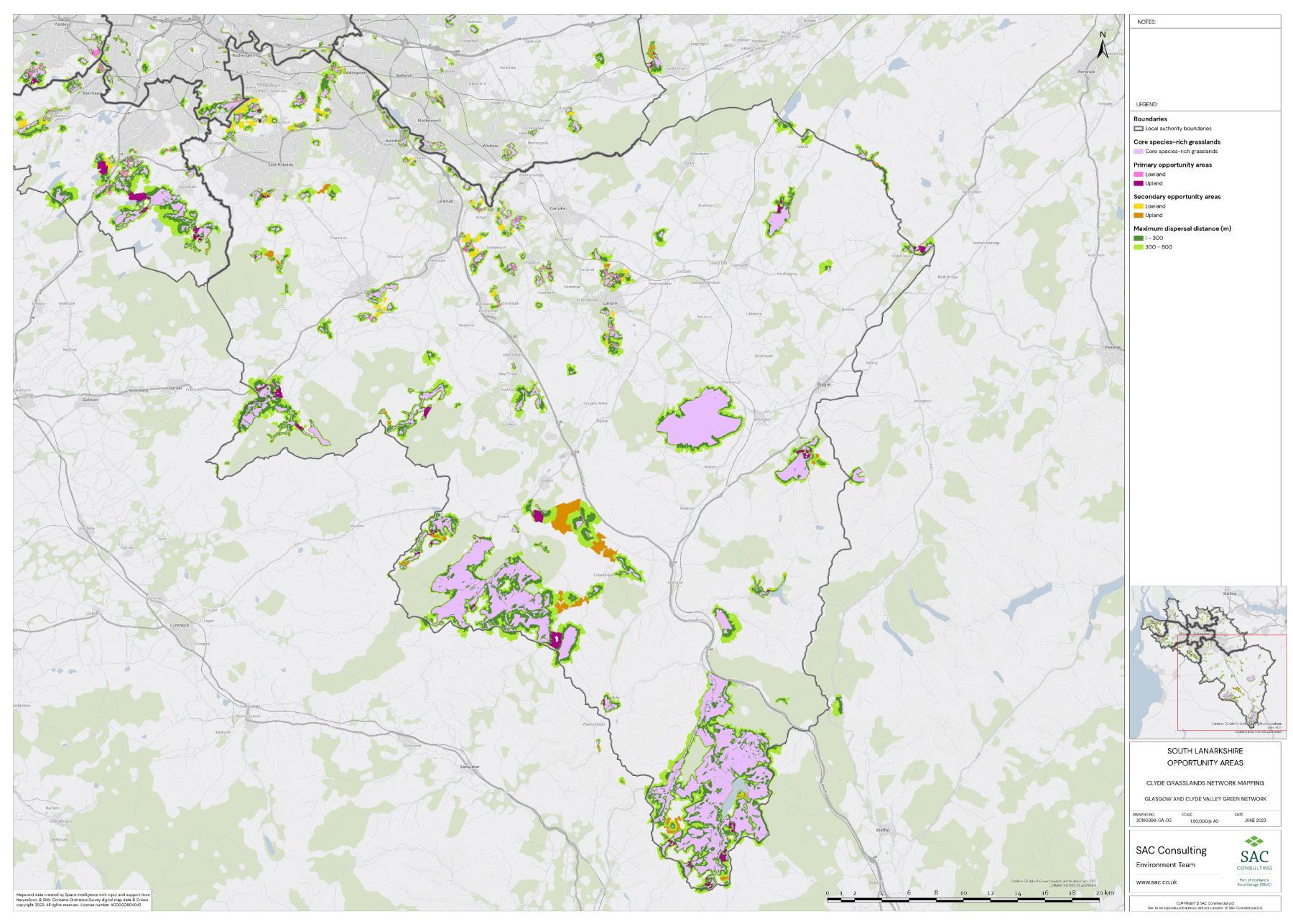
GCRGN: Mapping species-rich grassland networks
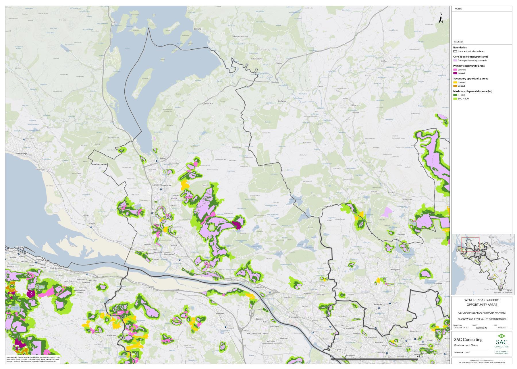
Table 17: Estimated costs associated with creating SRG on opportunity areas across each local authority. Each opportunity area provides a relatively large area within which SRG creation could enhance connectivity between network patches. On the ground habitat creation would be more focussed and involve smaller habitat pathces with the area selected depending on land use, land ownership and management. Costs are based on the entire area of primary and secondary opportunity areas and costs are therefore over-estimated Costs per hectare are provided for each option. Values do not include costs associated with loss of