
Chapter 2 Supply and Demand SOLUTIONS TO END-OF-CHAPTER QUESTIONS DEMAND

1.1 When the price of coffee changes, the change in the quantity demanded reflects a movement along the demand curve. When other variables that affect demand change, the entire demand curve shifts. For example, when income changes, this causes coffee demand to shift.
1.2
Q ∂ ∂ = 0.1.
Y
An increase in Y shifts the demand curve to the right, from D1 to D2.
1.3 The market demand curve is the sum of the quantity demanded by individual consumers at a given price. Graphically, the market demand curve is the horizontal sum of individual demand curves.

1.4
a. The inverse demand curve for other town residents is p = 200 – 0.5Qr.

b. At a price of $300, college students demand 100 units of firewood, and other residents demand no firewood. Other residents will demand zero units of firewood if the price is greater than or equal to $200.
c. The market demand curve is the horizontal sum of individual demand curves, as illustrated below.

2.1 The effect of a change in pf on Q is
= –20pf
= –20(1.10)
= –22 units.
Thus, an increase in the price of fertilizer will shift the avocado supply curve to the left by 22 units at every price (i.e., a parallel shift to the left).
2.2 When the price of avocados changes, the change in the quantity supplied reflects a movement along the supply curve. When costs or other variables that affect supply change, the entire supply curve shifts. For example, the price of fertilizer represents a key factor of avocado production, which affects the cost of avocado production, shifting the avocado supply curve. This is because avocado prices are measured on a graph axis. Other factors that affect supply are not measured by a graph axis.
2.3 Given the supply function,
Q = 58 + 15p – 20pf,
The effect of a change in p on Q is
= 15p
To change quantity by 60, price would need to change by 60 = 15p p = $4.00.
2.4 The market supply curve is the sum of the quantity supplied by individual producers at a given price. Graphically, the market supply curve is the horizontal sum of individual supply curves.


MARKET EQUILIBRIUM
3.1 The supply curve is upward sloping and intersects the vertical price axis at $6. The demand curve is downward sloping and intersects the vertical price axis at $4. When all market participants are able to buy or sell as much as they want, we say that the market is in equilibrium: a situation in which no participant wants to change its behavior. Graphically, a market equilibrium occurs where supply equals demand. An equilibrium does not occur at a positive quantity because supply does not equal demand at any price.
3.2 The equilibrium price is p = 20 and the equilibrium quantity is Q = 80.

3.3 Given that pc = $5 and Y = $55,000 (note Y is measured in thousands, so the value to use here is 55), the demand for coffee can be rewritten as
Q = 14 – p and the supply of coffee can be rewritten as
Q = 8.6 + 0.5p.
When all market participants are able to buy or sell as much as they want, we say that the market is in equilibrium: a situation in which no participant wants to change its behavior. Graphically, a market equilibrium occurs where supply equals demand. Thus, the equilibrium price is
D = S
14 – p = 8.6 + 0.5p 5.4 = 1.5p
p = $3.60.
Find the equilibrium quantity by substituting this price into either the supply or demand function. For example, using the supply function, the equilibrium quantity is
Q = 8.6 + 0.5p
Q = 8.6 + 0.5(3.60)
Q = 8.6 + 1.8
Q = 10.4 units.
SHOCKS TO THE EQUILIBRIUM
4.1 a. The new equilibrium with the horizontal supply curve is where the new demand curve intersects the horizontal supply curve. The new equilibrium price is unchanged. See figure.
b. The new equilibrium with the vertical supply curve is where the new demand curve intersects the vertical supply curve. The new equilibrium price is higher. See figure.
c. The new equilibrium with the upward-sloping supply curve is where the new demand curve intersects the upward-sloping supply curve. The new equilibrium price is higher. See figure.

4.2 a. Health benefits from drinking coffee shift the demand curve for coffee to the right because more coffee is now demanded at each price. The new market equilibrium is where the original supply curve intersects the new coffee demand curve, at a higher price and larger quantity.

b. An increase in the usefulness of cocoa will increase demand for cocoa. This will drive up the equilibrium price of cocoa. Since cocoa and coffee are likely substitutes, this will increase the demand for coffee. The new market equilibrium is where the original supply curve intersects the new coffee demand curve, at a higher price and higher quantity.

c. A recession shifts the demand curve for coffee to the left because less coffee is now demanded at each price. The new market equilibrium is where the original supply curve intersects the new coffee demand curve, at a lower price and lower quantity.

d. New technologies increasing yields shift the supply curve for coffee to the right because more coffee is now supplied at each price. The new market equilibrium is where the original demand curve intersects the new coffee supply curve, at a lower price and higher quantity.

4.3 Outsourcing shifts the labor demand curve to the right because more Indian workers are demanded at each wage. The new market equilibrium is where the original supply curve intersects the new labor demand curve.
4.4 Given that pt = $0.80, the demand for avocados can be rewritten as Q = 160 – 40p and the supply of avocados can be rewritten as Q = 50 + 15p.
When all market participants are able to buy or sell as much as they want, we say that the market is in equilibrium: a situation in which no participant wants to change its behavior. Graphically, a market equilibrium occurs where supply equals demand. Thus, the equilibrium price is
D = S
160 – 40p = 50 + 15p
110 = 55p
p = $2.00.
Find the equilibrium quantity by substituting this price into either the supply or demand function. For example, using the supply function, the equilibrium quantity is
Q = 50 + 15p
Q = 50 + 15(2.00)
Q = 50 + 30
Q = 80 units.
When the price of tomatoes increases to $1.35, the demand curve for avocados shifts out to
Q = 171 – 40p


conomics and Str

rategy,
Second
of avocados
s is unchang
The equilib
brium quantit


The numbe right by 11
rs suggest th percent, yet


171 – 4 1 p ty is found a Q = Q = 5 Q Q hat labor dem t the decreas

The damage decreasing
e reduces the the equilibri


©2017
40p = 50 + 1
21 = 55p = $2.20.
as before 50 + 15p 50 + 15(2.20 = 50 + 33 = 83 units.
w equilibrium
m is found w
15p 0)
mand is inela e in equilibr
astic. The su rium wage is
upply curve s s only 3.2 pe
where shifts to the ercent.
reasing the e uice.
Edition n, Inc.
equilibrium p
price and
The demand for grapefruit juice increases as the price of orange juice increases because grapefruit juice is a substitute. As the demand for grapefruit juice increases, the equilibrium price and quantity of grapefruit juice increase.

4.7 The increased use of corn for producing ethanol will shift the demand curve for corn to the right. This increases the price of corn overall, reducing the consumption of corn as food.

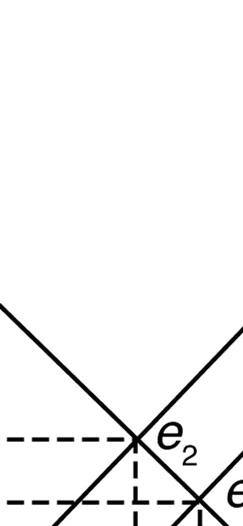
4.8 Suppose supply is initially S1, but it decreases by a small amount to S2 after the BP oil spill. When all market participants are able to buy or sell as much as they want, we say that the market is in equilibrium: a situation in which no participant wants to change its behavior. Graphically, a market equilibrium occurs where supply equals demand. The original market equilibrium is where the original demand curve intersects the original supply curve (e1). The new market equilibrium is where the original demand curve intersects the new supply curve (e2). When the supply curve shifts by a relatively small amount, the change in the equilibrium price is likely to be small.


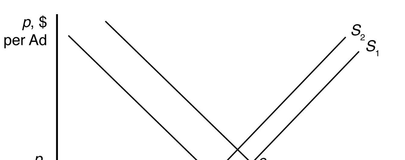
4.9 The Internet shifts the demand curve for newspaper advertising to the left because fewer companies demand newspaper advertising with online advertising available. The Internet may force some newspapers out of business, so the supply curve for newspaper advertising will shift to the left some. The new market equilibrium is where the new demand curve intersects the new supply curve. At the new equilibrium, there is less newspaper advertising.

4.10 If global warming causes both an increase in the supply of wine during a period of time when the demand for wine is also rising, then the overall effect on the equilibrium quantity of wine will be for the quantity to increase. This is true because both the increase in supply (from S1 to S2 or S3) and the increase in demand (from D1 to D2) will result in higher equilibrium quantities on their own, and so the combination of the two effects will definitely be an increase in quantity. The effect of these events on the equilibrium price of wine, however, is indeterminate. The increase in demand will lead to a higher equilibrium price, but the increase in supply will lead to a lower equilibrium price. Taken together, the net effect on price will be determined by how large the shifts of supply and demand are relative to one another. If the supply shift is larger (from S1 to S2), then price will fall. If, on the other hand, the demand shift is larger, then price will rise.

4.11 An increase in petroleum prices shifts the aluminum supply curve to the left because the cost of producing aluminum is more expensive at each price. An increase in the cost of petroleum also shifts the demand curve for aluminum to the right because the petroleum price increase makes a substitute, plastic, more expensive (by making the cost of plastic production higher). The new equilibrium is where the new aluminum supply curve intersects the new aluminum demand curve.
When the supply curve shifts to the left, the new equilibrium price is higher, and the new equilibrium quantity is lower. When the demand curve shifts to the right, the new equilibrium price is higher, and the new equilibrium quantity is higher. When both curves shift, the new equilibrium price is higher, but the new equilibrium quantity could be higher, lower, or unchanged.


4.12 The cartoon seems to show a bumper harvest of lobsters. A large increase in the catch will shift the supply curve to the right (from S1 to S2), which will cause price to fall from p1 to p2

Solution
ns
Manual—Cha
apter 2/Supply an
nd Demand 11
13
EFFE 5.1
ECTS OF G
GOVERNME
ENT INTER
RVENTION
5.2
Requiring o fewer peopl equilibrium curve, at a h


In the absen Hurricane K from q0 to q want to pur resulting sh off. The red
occupational le are able to m is where th higher wage nce of price Katrina woul q1. At a gove rchase q d uni hortage woul duced quanti
l licenses shi o supply thei he original de and lower e controls, the ld push mark ernment imp its, but produ ld impose se ity and price
ifts the labor ir labor at ea emand curve employment e leftward sh ket prices up posed maxim ucers would earch costs o e also reduce
hift of the sup p from p0 to p mum price of only be will n consumers e firms’ profi
ve to the left he new mark he new labo pply curve a p1 and reduc f p2, consum ling to sell q s, making th fits.
t because ket or supply as a result of ce quantity mers would s units. The hem worse
5.3
With a bind loans, some obtain them bank loans
ding price ce e consumers m. This is bec to low-incom
eiling, such a who deman cause the dem me househol
on the rate th he rate ceilin ank loans is g usury law.
f of
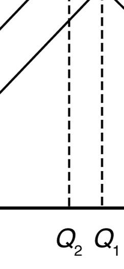
5.4 With the binding rent ceiling, the quantity of rental dwellings demanded is that quantity where the rent ceiling intersects the demand curve (QD). The quantity of rental dwellings supplied is that quantity where the rent ceiling intersects the supply curve (QS). With the rent control laws, the quantity supplied is less than the quantity demanded, so there is a shortage of rental dwellings.

5.5 We can determine how the total wage payment, W = wL(w), varies with respect to w by differentiating. We then use algebra to express this result in terms of an elasticity:
whereε is the elasticity of demand of labor. The sign of dW/dw is the same as that of 1 + ε. Thus total labor payment decreases as the minimum wage forces up the wage if labor demand is elastic, ε<–1, and increases if labor demand is inelastic, ε>–1.

For a graphical explanation, see the figures below. In the top panel with very flat supply and demand curves, the imposition of a minimum wage causes overall wage payments to fall dramatically. On the other hand, when supply and demand curves are steep (as in the bottom panel) overall wage payments increase substantially.

5.6 Before the tax is imposed, the demand for avocados can be rewritten as
Q = 160 – 40p and the supply of avocados is given as
Q = 50 + 15p.
When all market participants are able to buy or sell as much as they want, we say that the market is in equilibrium: a situation in which no participant wants to change its behavior. Graphically, a market equilibrium occurs where supply equals demand. Thus, the equilibrium price is
D = S
160 – 40p = 50 + 15p
110 = 55p
p = $2.00.
Find the equilibrium quantity by substituting this price into either the supply or demand function. For example, using the supply function, the equilibrium quantity is
Q = 50 + 15p
Q = 50 + 15(2.0)
Q = 50 + 30
Q = 80 units.
If a $0.55 tax is imposed, the demand curve can be rewritten to account for the tax. First, the demand curve can be rewritten as inverse demand by solving for p
Q = 160 – 40p
p = 4 – 0.025Q.
The tax is subtracted from inverse demand to give p = 3.45 – 0.025Q and then this inverse demand curve can be turned back into a demand curve
Q = 138 – 40p
Setting supply equal to demand, the new equilibrium (pretax) price is
D = S
138 – 40p = 50 + 15p
88 = 55p
p = $1.60.
The after-tax price is $2.15.