
Generalization of the Dependent Function in Extenics for Nested Sets with Common Endpoints to 2D-Space, 3D-Space, and generally to n-D-Space
Florentin Smarandache University of New Mexico Mathematics and Science Department 705 Gurey Ave. Gallup, NM 87301, USA E-mail: smarand@unm.edu
Abstract.
In this paper we extend Prof. Yang Chunyan and Prof. Cai Wen’s dependent function of a point P with respect to two nested sets X0 ⊂ X, for the case the sets X0 and X have common ending points, from 1D space to n-D-space. We give several examples in 2D- and 3D-spaces. When computing the dependent function value k(.) of the optimal point O, we take its maximum possible value. Formulas for computing k(O), and the geometrical determination the Critical Zone are also given.
1. Principle of Dependent Function of a point P(x) with respect to a nest of two sets X0 ⊂ X, i.e. the degree of dependence of point P with respect to the nest of the sets X0 ⊂ X, is the following. The dependent function value, k(x), is computed as follows: the extension distance between the point P and the larger set’s closest frontier, divided by the extension distance between the frontiers of the two sets {both extension distances are taken on the line/geodesic that passes through the point P and the optimal/attracting point O}; the dependent function value is positive if point P belongs to the larger set, and negative if point P is outside of the larger set.
2. Dependent Function Formula for nested sets having common ending points in 1D-Space.
For two nested sets X0 ⊂ X from the one-dimensional space of real numbers R, with X0 and X having common endpoints, the Dependent Function K(x), which gives the degree of dependence of a point x with respect to this pair of included 1D-intervals, was defined by Yang Chunyan and Cai Wen in [2] as:
3. n-D-Dependent Function Formula for two nested sets having no common ending points The extension n-D-dependent function k(.) of a point P, which represents the degree of dependence of the point P with respect to the nest of the two sets X0 ⊂ X, is:
kP
(,)(,)|||| () (,)(,)(,)(,)||||||
02112
(2) In other words, the extension n-D-dependent function k(.) of a point P is the n-D-extension distance between the point P and the closest frontier of the larger set X, divided by the n-Dextension distance between the frontiers of the two nested sets X and X0; all these n-Dextension distances are taken along the line (or geodesic) OP
4. n-D-Dependent Function Formula for two nested sets having common ending points.
extension 2D-distance, and then we compute the extension 2D-dependent function. Let’s do an extension 2D-diagram: y (-2, -∞) R A1 A(0,22) (-1,0) P2 D(32,22) A’(2,21) P1 D’(32,21) P (-1,0) O(17,11) Q Q1 Q2 B’(2,1) C’(32,1) B1 B(0,0) (-1,0) C(32,0) S
Diagram 1.
The Critical Zone in the top, down, and left sides of the Diagram 1 as the same as for the case when the two pink and black rectangles have no common ending points. But on the right-hand side the Critical Zone is delimitated by the a blue curve in the middle and the blue dotted lines in the upper and lower big rectangle’s corners. The dependent function of the points Q, Q1, Q2 is respectively: k(Q) = |QQ1|+1, and k(Q1) = 1 (if Q1 ∈ A’B’C’D’) or 0 (if Q1 ∉ A’B’C’D’), and k(Q2) = -|Q2Q1|= -1, (4) where |MN| means the geometrical distance between the points M and N. The dependent function of point P is normally computing: 2 12
|| () || PP kP PP = . (5)
5.2. Example 2 of nested rectangles with two common sides. y (-1,0) A1 (-1,0) A A’ T1 P’ C’ T3 (-1,0) T5 T4 O P T2 (-1, 0) B’(2,1) T6 C’(32,1) (-1,0) B1 B(0,0) T7 (-1,0) C(32,0) S
Diagram 2.
We observe that the Critical Zone changes dramatically in the places where the common ending points occur, i.e. on the top and respectively left -hand sides. The Critical Zone is delimitated by blue curves and lines on the top and respectively left-hand sides. Now, the dependent function of point P is different from the Diagram 1: k(P)=|PP’|+1. (6) The dependent function of the optimal point O should be the maximum possible value. Therefore, k(O) = max {|OT1|+1, |OT2|+1, |OP’|+1, |OC’|+1, 7 67
|| || OT TT , 5 45
|| || OT TT , 3
|| || OA TA , etc. }. (7)
5.3. Example 3 of nested circles with one common ending point. Assume the desirable circular factory piece radius is 6 cm and acceptable is 8 cm, but they have a common ending point P’.
Diagram 3.
The Critical Zone is between the green and blue circles, together with the blue line segment P’’P’ (this line segment resulted from the fact the P’ is a common ending point of the red and green circles).
The dependent function values for the following points are: k(P) =|PP’|+1; (8) k(P’) = 1 (if P’ belongs to the red circle), or 0 (if P’ does not belong to the red circle); (9) k(P’’) = |P’’P’|; (10) k(O) = max {|OP’|+1; 4 34
|| || OT TT , (11) where T3 lies arbitrary on the red circle, but T3 ≠ P’, and T4 lies on the green circle but T4 belongs to the line (or geodesic) OT3}.
5.4. Example 4 of nested triangles with one common bottom side.
Diagram 4.
The Critical Zone is between the green and blue dotted triangle to the left-hand and right-hand sides, while at the bottom side the Critical Zone is delimitated by the blue curve in the middle and the blue small oval triangles A’’AA’ and respectively B’’BB’.
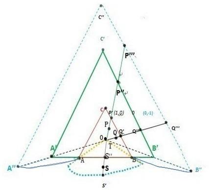
The dependent function values of th e following points are given below: |''| ()1; |'''| PP kP PP => k(P’)=1; k(P’’)=0; k(P’’’) = -1. (12) Similarly: |''| ()1; |'''| QQ kQ QQ => k(Q’)=1; k(Q’’)=0; k(Q’’’) = -1. (13)
With respect to the bottom common side (where the line segment AB lies on line segment A’B’) one has: k(T) = |TS’’|+1; k(S’’) = 1 (if S’’ belongs to the red triangle ABC), or 0 (if S’’ does not belong to the red triangle ABC); k(S) = |SS’’|; k(S’) = -1. (14)
The Critical Zone (the zone where the extension dependent function takes values between 0 and -1) envelopes the larger green prism ABCDEFGH at an equal distance from it as the distance between the red prism A’B’C’D’E’F’G’H’ and the green prism ABCDEFGH with respect to the faces ABCD, ADHE, BCGF, EFGH, and ABFE (because these green faces and their corresponding
red faces A’B’C’D’, A’D’H’E’, B’C’G’F’, E’F’G’H’, and respectively A’B’F’E’ have no common points).
But the green face DCGH contains the red face D’C’G’H’, therefore for all their common points (i.e. all points inside of and on the rectangle D’C’G’H’) the extension dependent function has wild values. D’C’G’H’ entirely lies on DCGH. The Critical Zone related to the right-hand green face DCGH and the red face D’C’G’H’ is the solid bounded by the blue continuous and dashed curves on the right-hand side.
In general, let’s consider two n-D sets, S1 ⊂ S2, that have common ending points (on their frontiers). Let’s note by CE their common ending point zone. Then:
The Dependent Function Formula for computing the value of the Optimal Point O is
OP PP ∈−∈− ∈
|''| max() |'''| E E P FrSCPFrSC POP OPPlinegeodesic
k(O) = max { '' max(|''|1) SCE OS ∈ + ; 12 '(),''() ''' ''/
∈
}. (16) We can define the Critical Zone in the sides where there are common ending points as: ZC1 = {P(x)|P ∈ U-S2, 0 < d(P,P’’) ≤ 1, P’’ ∈ Fr(S1) ∩ Fr(S2) and P’’ ∈ OP}, (17) where d(P,P’’) is the classical geometrical distance between the points P and P’’. And for the sides which have no common ending points, the Critical Zone is: ZC2 = {P(x)|P ∈ U-S2, 0 < d(P,P’’) ≤ d(P’’P’), where P’’ ∈ Fr(S2) and P’ ∈ Fr(S1) and P’’OP}. (18) Whence, the total Critical Zone is: ZC = ZC1 ∪ ZC2. (19)
References:
[1] Cai Wen. Extension Set and Non-Compatible Proble ms [J]. Journal of Scientific Exploration, 1983, (1): 83-97.
[2] Yang Chunyan, Cai Wen. Extension Engineering [M]. Beijing: Public Library of Science, 2007.
[3] F. Smarandache, Generalizations of the Distance and Dependent Function in Extenics to 2D, 3D, and n-D, viXra.org, http://vixra.org/abs/1206.0014 and http://vixra.org/pdf/1206.0014v1.pdf, 2012
[4] F. Smarandache, V. Vlădăreanu, Applications of Extenics to 2D-Space and 3D-Space, viXra.org, http://vixra.org/abs/1206.0043 and http://vixra.org/pdf/1206.0043v2.pdf, 2012.