Chapter 2
Supply and Demand
1.1 When the price of avocados changes, the change in the quantity demanded reflects a movement along the demand curve. When other variables that affect demand change, the entire demand curve shifts. For example, when income changes, this causes avocado demand to shift.

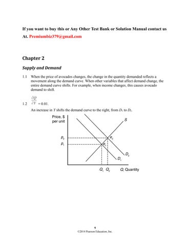
1.2 = 0.01.
An increase in Y shifts the demand curve to the right, from D1 to D2.
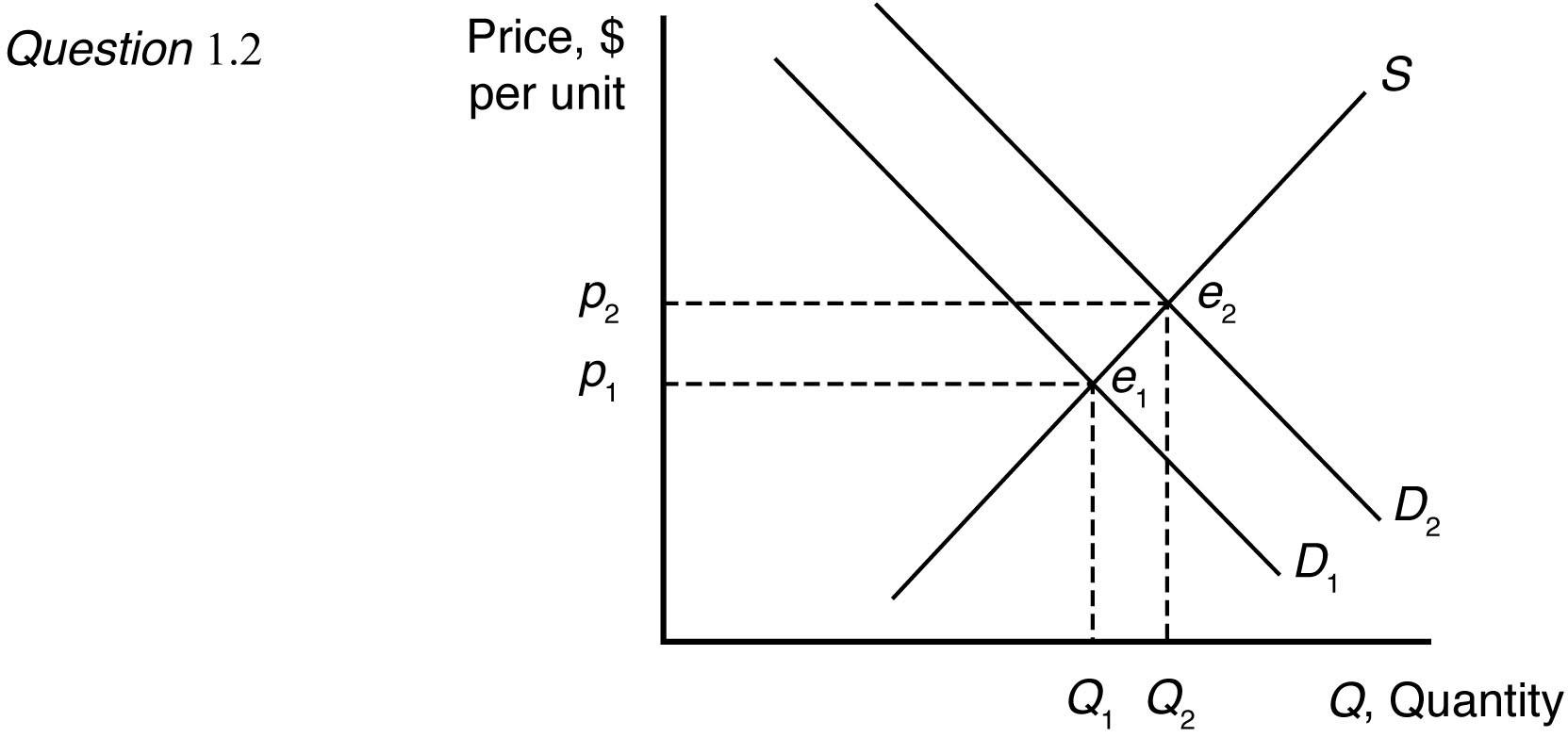
1.3 The market demand curve is the sum of the quantity demanded by individual consumers at a given price. Graphically, the market demand curve is the horizontal sum of individual demand curves.
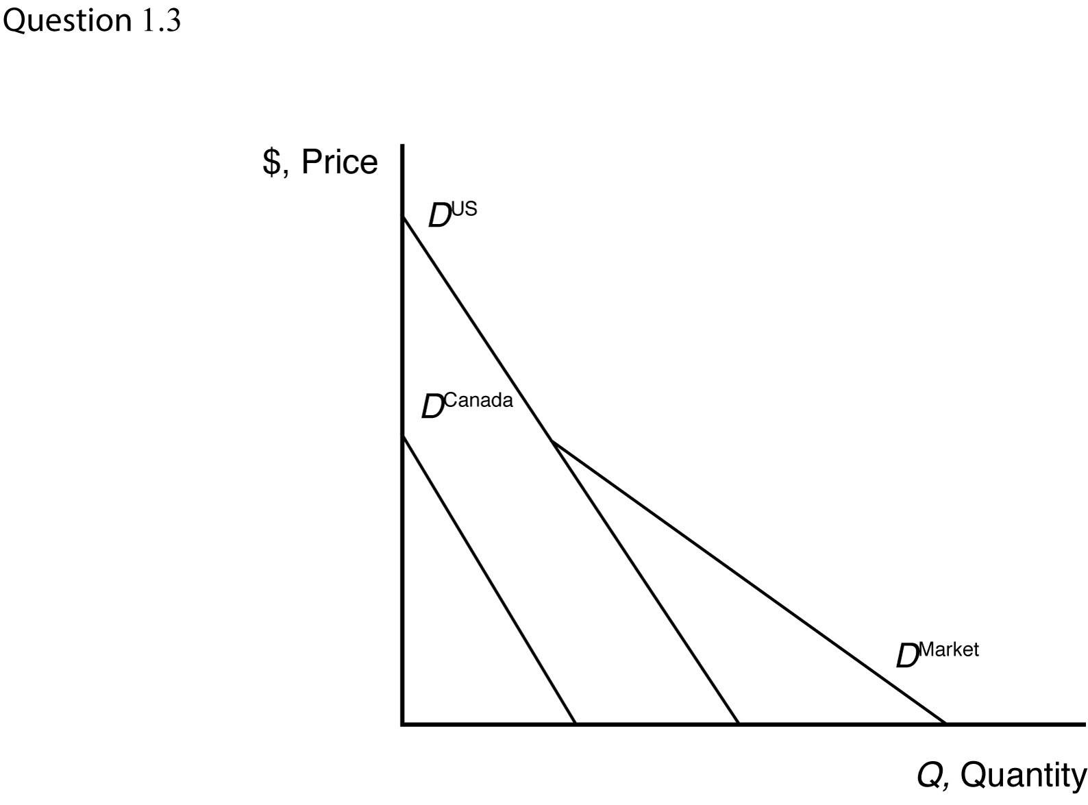
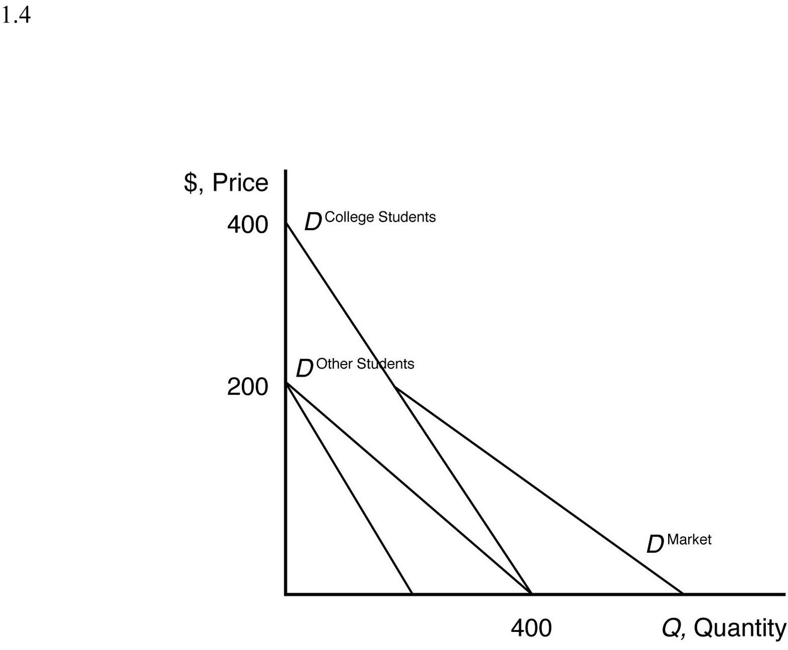
1.4 The inverse demand curve for other town residents is p = 200 – 0.5Q . At a price of $300, college students demand 100 units of firewood, and other residents demand no firewood. Other residents will demand zero units of firewood if the price is greater than or equal to $200. The market demand curve is the horizontal sum of individual demand curves, as
2.1 The effect of a change in pf on Q is = –20pf = –20(1.10) = –22 units.

Thus, an increase in the price of fertilizer will shift the avocado supply curve to the left.
2.2 When the price of avocados changes, the change in the quantity supplied reflects a movement along the supply curve. When costs or other variables that affect supply change, the entire supply curve shifts. For example, the price of fertilizer represents a key factor of avocado production, which affects the cost of avocado production, shifting the avocado supply curve. This is because avocado prices are measured on a graph axis. Other factors that affect supply are not measured by a graph axis.
2.3 Given the supply function, Q = 58 + 15p–20pf,
The effect of a change in p on Q is = 15p.

To change quantity by 60, price would need to change by 60 = 15p p = $4.00.
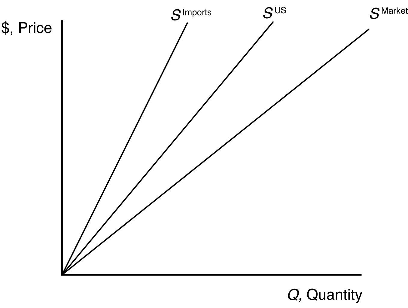
2.4 The market supply curve is the sum of the quantity supplied by individual producers at a given price. Graphically, the market supply curve is the horizontal sum of individual supply curves.
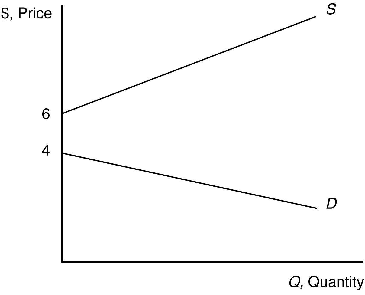
3.1 The supply curve is upward sloping and intersects the vertical price axis at $6. The demand curve is downward sloping and intersects the vertical price axis at $4. When all market participants are able to buy or sell as much as they want, we say that the market is in equilibrium: a situation in which no participant wants to change its behavior. Graphically, a market equilibrium occurs where supply equals demand. An equilibrium does not occur at a positive quantity because supply does not equal demand at any price.
3.2 The equilibrium price is p = 20 and the equilibrium quantity is Q = 80.
©2014 Pearson Education, Inc.
3.3
Given that pt = $0.80, Y = $4,000, and pf = $0.40, the demand for avocados can be rewritten as
Q = 160 – 40p and the supply of avocados can be rewritten as
Q = 50 + 15p.
When all market participants are able to buy or sell as much as they want, we say that the market is in equilibrium: a situation in which no participant wants to change its behavior. Graphically, a market equilibrium occurs where supply equals demand. Thus, the equilibrium price is
D = S
160 – 40p = 50 + 15p 132 = 55p p = $2.40.
Find the equilibrium quantity by substituting this price into either the supply or demand function. For example, using the supply function, the equilibrium quantity is
Q = 50 + 15p
Q = 50 + 15(2.40)
Q = 50 + 26
Q = 76 units.
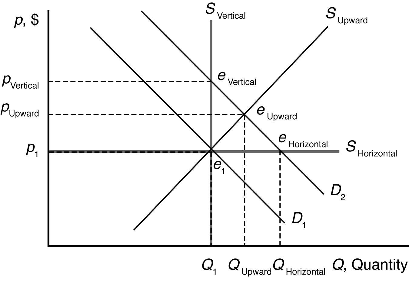
4.1 The demand curve shifts to the right. The new equilibrium with the horizontal supply curve is where the new demand curve intersects the horizontal supply curve. The new equilibrium with the vertical supply curve is where the new demand curve intersects the vertical supply curve. The new equilibrium with the upward-sloping supply curve is where the new demand curve intersects the upward-sloping supply curve. The new equilibrium price is higher with the vertical and upward-sloping supply curves but unchanged with the horizontal supply curve.
©2014 Pearson Education, Inc.
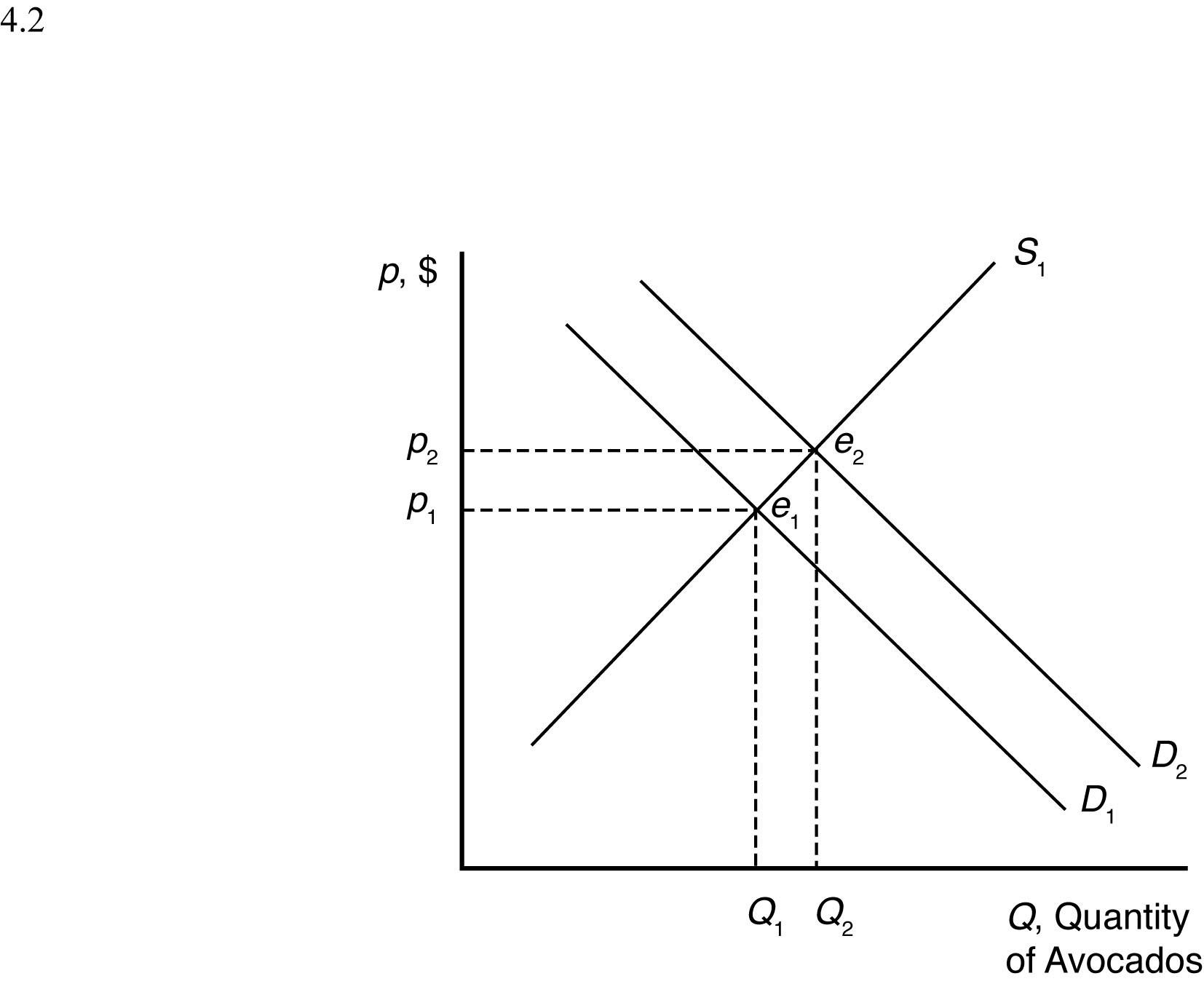
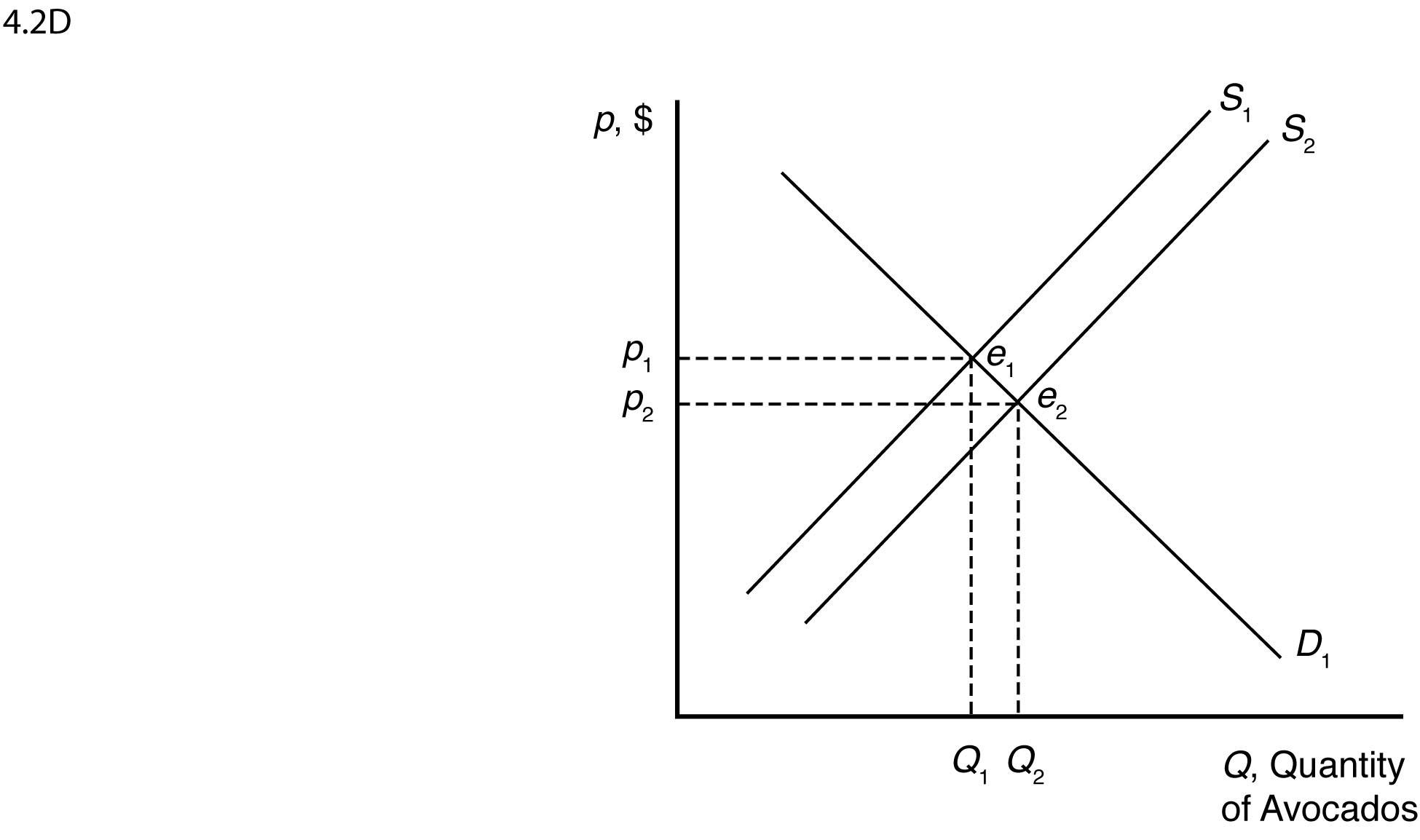
4.2 Health benefits from eating avocados shift the demand curve for avocados to the right because more avocados are now demanded at each price. The new market equilibrium is where the original supply curve intersects the new avocado demand curve, at a higher price
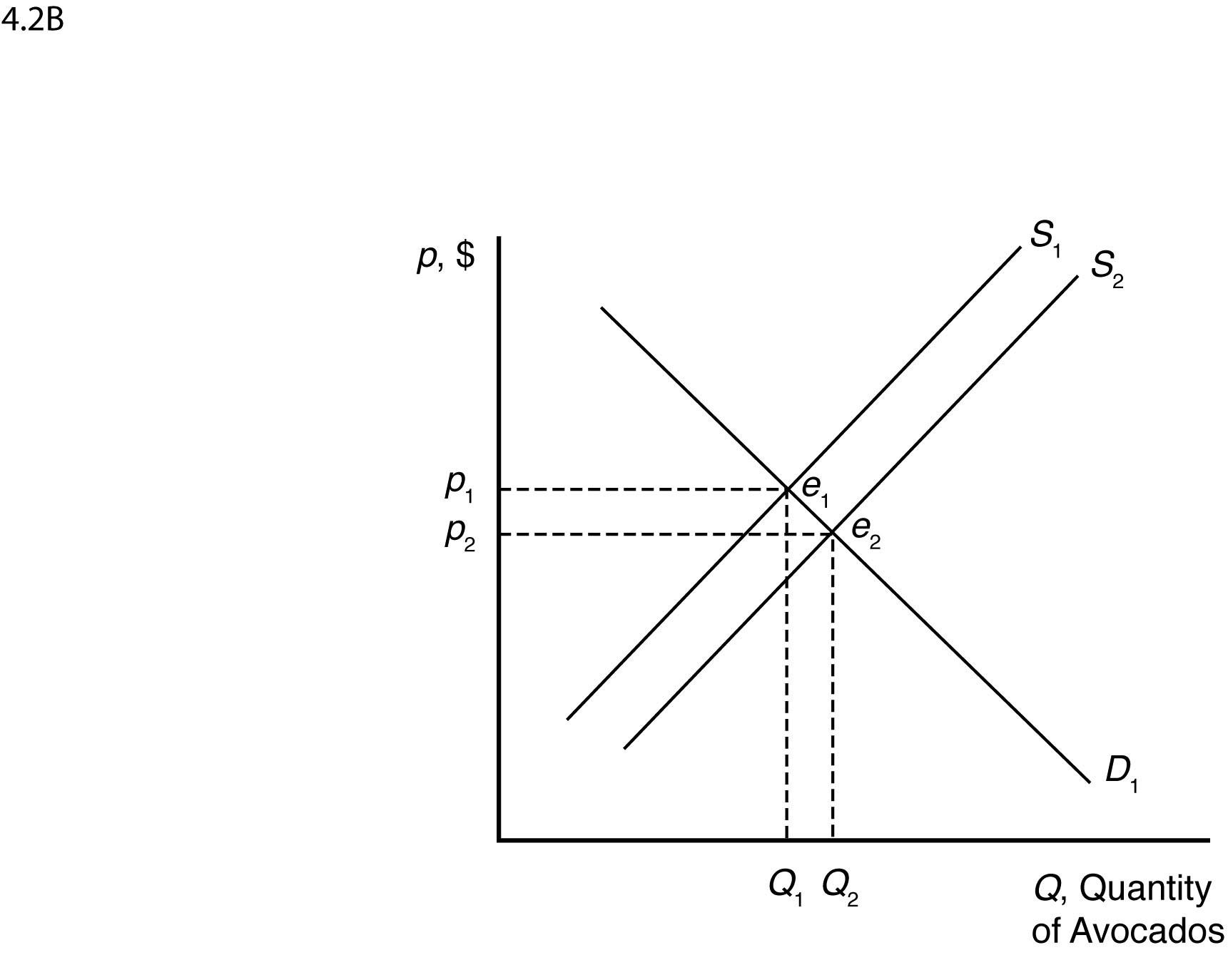
Imports shift the supply curve for avocados to the right because more avocados are now supplied at each price. The new market equilibrium is where the original demand curve intersects the new avocado supply curve, at a lower price and higher quantity.
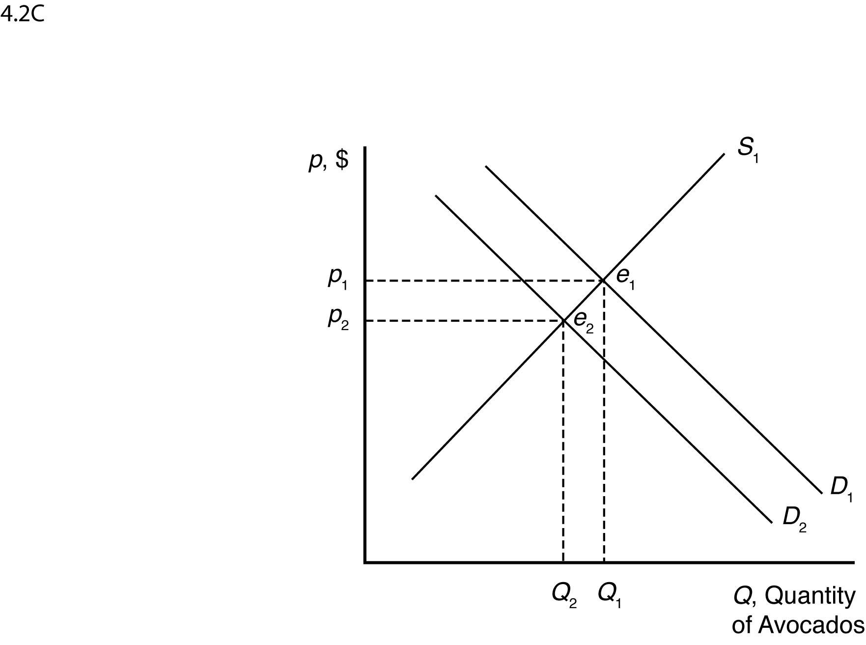
A recession shifts the demand curve for avocados to the left because fewer avocados are now demanded at each price. The new market equilibrium is where the original supply curve intersects the new avocado demand curve, at a lower price and lower quantity.
New technologies increasing yields shift the supply curve for avocados to the right because more avocados are now supplied at each price. The new market equilibrium is where the original demand curve intersects the new avocado supply curve, at a lower price and higher
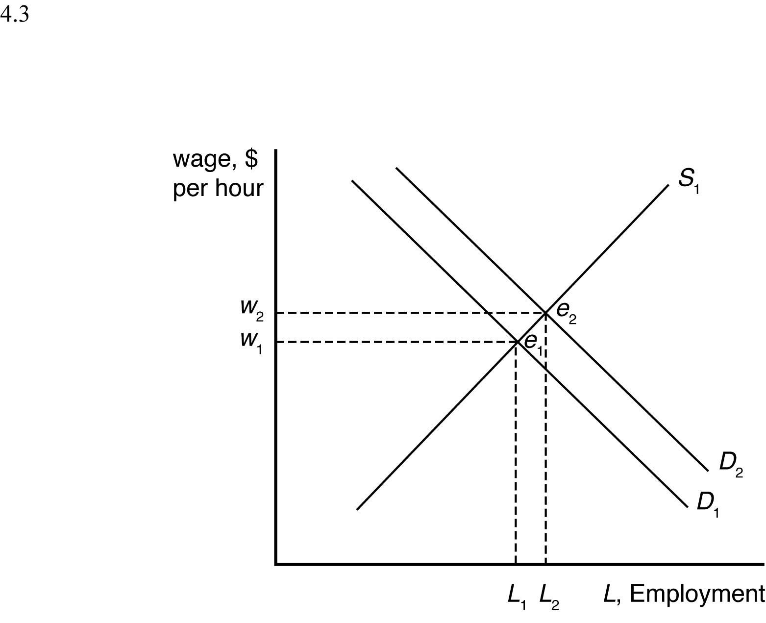
4.3 Outsourcing shifts the labor demand curve to the right because more Indian workers are demanded at each wage. The new market equilibrium is where the original supply curve
4.4 Given that pt = $1.35, Y = $4,000, and pf = $0.95, the demand for avocados can be rewritten as
Q = 171 – 40p and the supply of avocados can be rewritten as Q = 39 + 15p.
When all market participants are able to buy or sell as much as they want, we say that the market is in equilibrium: a situation in which no participant wants to change its behavior. Graphically, a market equilibrium occurs where supply equals demand. Thus, the equilibrium price is
D = S
171 – 40p = 39 + 15p
132 = 55p p = $2.40.
Find the equilibrium quantity by substituting this price into either the supply or demand function. For example, using the supply function, the equilibrium quantity is
Q = 39 + 15p
Q = 39 + 15(2.40)
Q = 39 + 36
Q = 75 units.
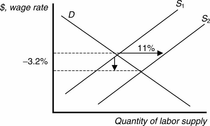
4.5 The numbers suggest that labor demand is inelastic. The supply curve shifts to the right by 11 percent, yet the decrease in equilibrium wage is only 3.2 percent.
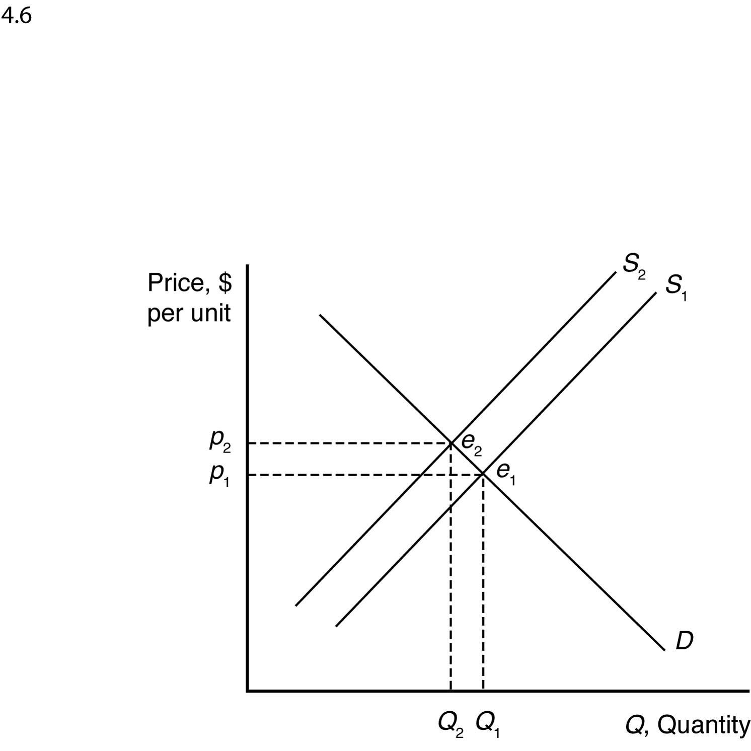
4.6 The damage reduces the supply of oranges, increasing the equilibrium price and decreasing the equilibrium quantity of orange juice.
©2014 Pearson Education, Inc.
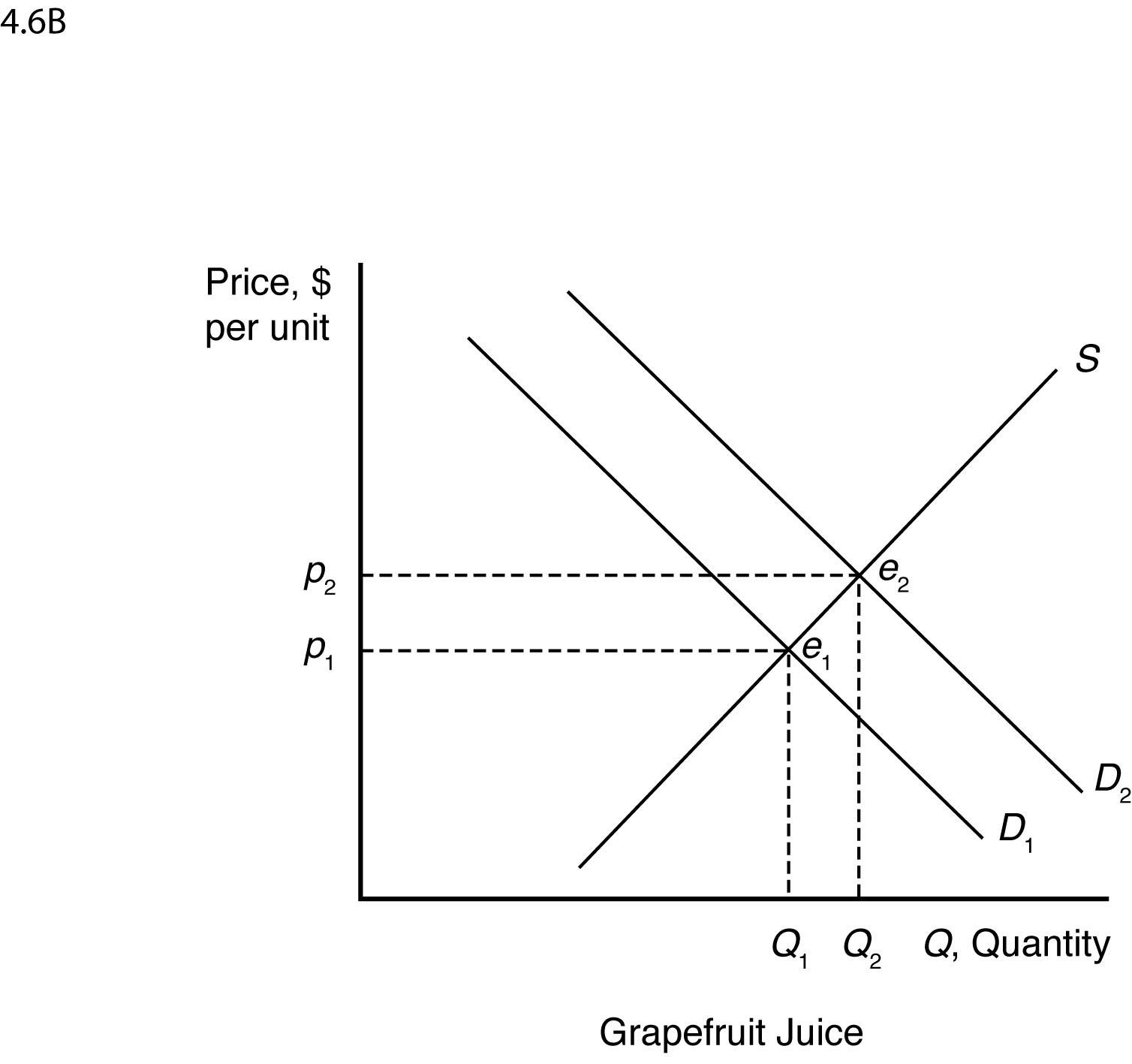
The demand for grapefruit juice increases as the price of orange juice increases because grapefruit juice is a substitute. As the demand for grapefruit juice increases, the equilibrium
4.7 The increased use of corn for producing ethanol will shift the demand curve for corn to the right. This increases the price of corn overall, reducing the consumption of corn as food.
©2014 Pearson Education, Inc.
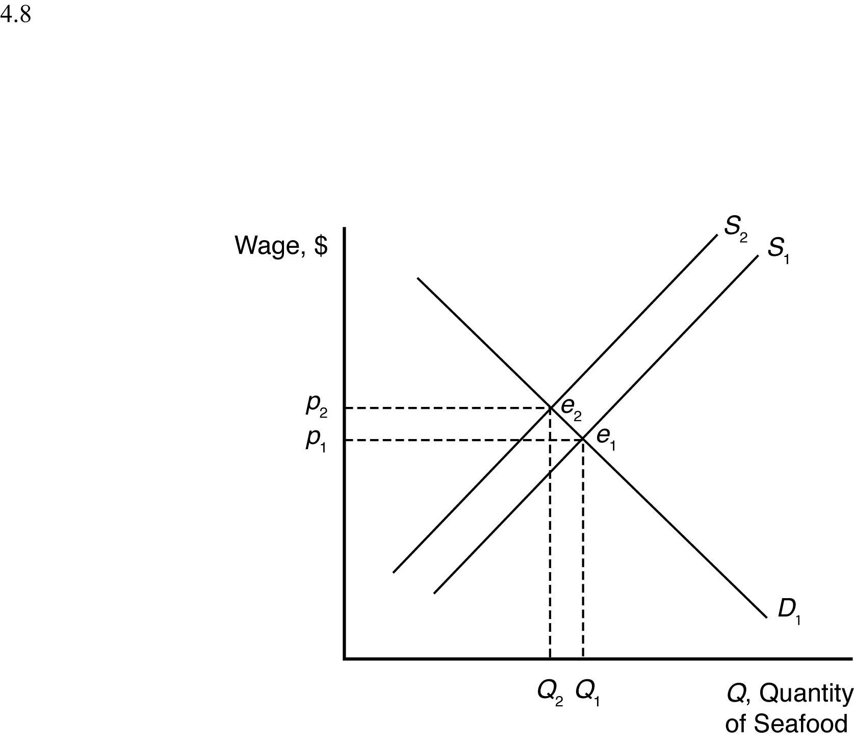
4.8 Suppose supply is initially S1, but it decreases by a small amount to S2 after the BP oil spill. When all market participants are able to buy or sell as much as they want, we say that the market is in equilibrium: a situation in which no participant wants to change its behavior. Graphically, a market equilibrium occurs where supply equals demand. The original market equilibrium is where the original demand curve intersects the original supply curve ). The new market equilibrium is where the original demand curve intersects the new ). When the supply curve shifts by a relatively small amount, the change in
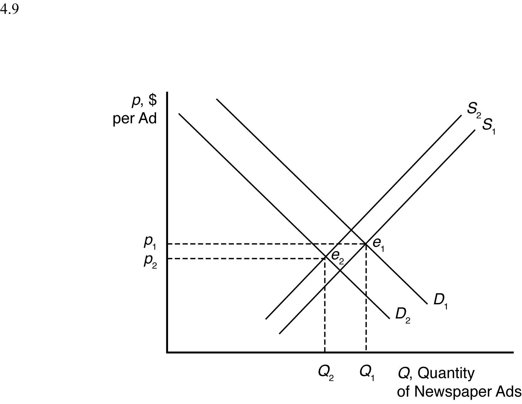
4.9 The Internet shifts the demand curve for newspaper advertising to the left because fewer companies demand newspaper advertising with online advertising available. The Internet may force some newspapers out of business, so the supply curve for newspaper advertising will shift to the left some. The new market equilibrium is where the new demand curve intersects the new supply curve. At the new equilibrium, there is less newspaper
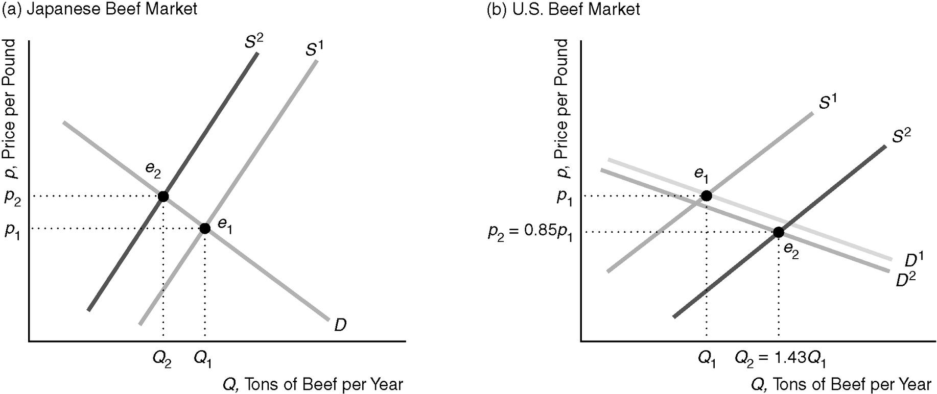
4.10 When Japan banned U.S. imports, the supply curve of beef in Japan shifted to the left from S1 to S2 in panel (a) of the figure. (The figure shows a parallel shift, for the sake of simplicity.) Presumably, the Japanese demand curve, D, was unaffected as Japanese consumers had no increased risk of consuming tainted meat. Thus, the shift of the supply curve caused the equilibrium to move along the demand curve from e1 to e2. The equilibrium price rose from p1 to p2 and the equilibrium quantity fell from Q1 to Q2. U.S. beef consumers’ fear of mad cow disease caused their demand curve in panel (b) of the figure to shift slightly to the left from D1 to D2. In the short run, total U.S. production was essentially unchanged. Because of the ban on exports, beef that would have been sold in Japan and elsewhere was sold in the United States, causing the U.S. supply curve to shift to the right from S1 to S2. As a result, the U.S. equilibrium changed from e1 (where S1 intersects D1) to e2 (where S2 intersects D2). The U.S. price fell 15 percent from p1 to p2 = 0.85p1, while the quantity rose 43 percent from Q1 to Q2 = 1.43Q1.
Note: Depending on exactly how the U.S. supply and demand curves had shifted, it would have been possible for the U.S. price and quantity to have both fallen. For example, if D2 had shifted far enough left, it could have intersected S2 to the left of Q1, so that the equilibrium quantity would have fallen. ©2014 Pearson Education,
4.11 If the demand curve had shifted to the left more than the supply curve shifted to the right, then the equilibrium quantity would have fallen. Under no circumstances could the equilibrium price increase, given the direction of the shifts, because the leftward shift in demand and the rightward shift in supply work together to lower the equilibrium price.
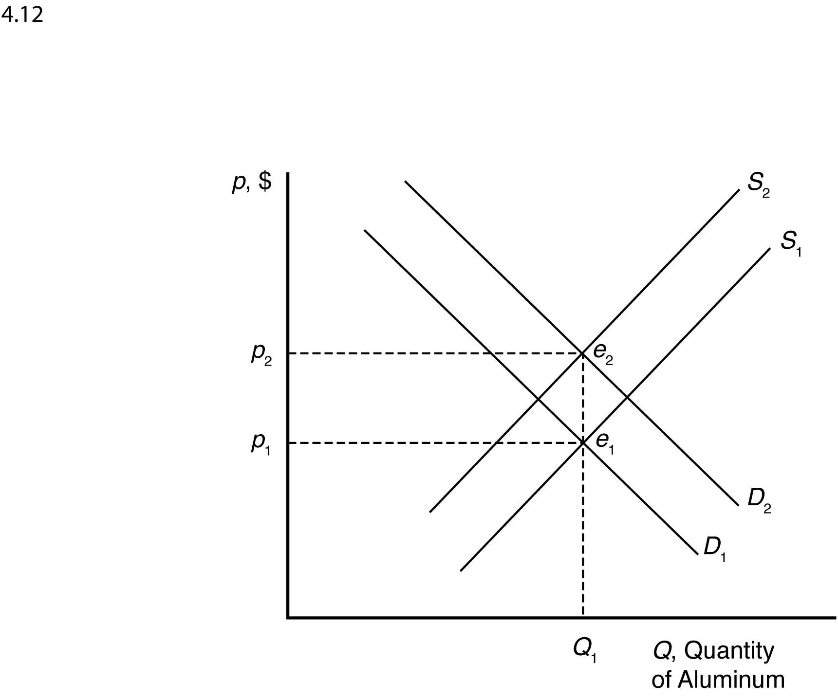
4.12 An increase in petroleum prices shifts the aluminum supply curve to the left because the cost of producing aluminum is more expensive at each price. An increase in the cost of petroleum also shifts the demand curve for aluminum to the right because the petroleum price increase makes a substitute, plastic, more expensive (by making the cost of plastic production higher). The new equilibrium is where the new aluminum supply curve intersects the new aluminum demand curve.
When the supply curve shifts to the left, the new equilibrium price is higher and the new equilibrium quantity is lower. When the demand curve shifts to the right, the new equilibrium price is higher and the new equilibrium quantity is higher. When both curves shift, the new equilibrium price is higher but the new equilibrium quantity could be higher, lower, or unchanged.
5.1 Requiring occupational licenses shifts the labor supply curve to the left because fewer people are able to supply their labor at each wage. The new market equilibrium is where the original demand curve intersects the new labor supply curve, at a higher wage and lower employment level.
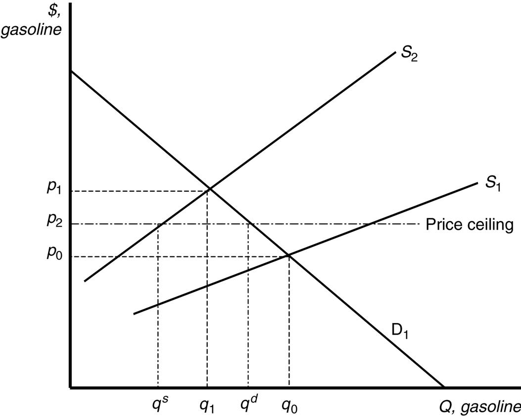
5.2 In the absence of price controls, the leftward shift of the supply curve as a result of Hurricane Katrina would push market prices up from p0 to p1 and reduce quantity from q0 to q1. At a government imposed maximum price of p2, consumers would want to purchase qd units but producers would only be willing to sell qs units. The resulting shortage would impose search costs on consumers making them worse off. The reduced quantity and price also reduced firms’ profits.
5.3 With a binding price ceiling, such as a ceiling on the rate that can be charged on loans, some consumers who demand loans at the rate ceiling will be unable to obtain them. This is because the demand for bank loans is greater than the supply of bank loans to low-income households with the usury law.
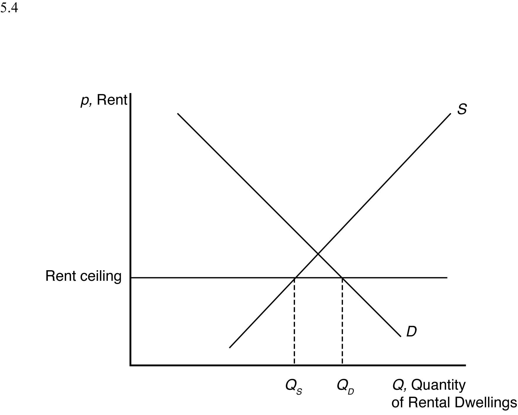
5.4 With the binding rent ceiling, the quantity of rental dwellings demanded is that quantity ). The quantity of rental dwellings ). With the rent control laws, the quantity supplied is less than the quantity demanded, so there is a
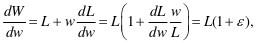
5.5 We can determine how the total wage payment, W = wL(w), varies with respect to w by differentiating. We then use algebra to express this result in terms of an elasticity: where is the elasticity of demand of labor. The sign of dW/dw is the same as that of 1 + . Thus total labor payment decreases as the minimum wage forces up the wage if labor demand is elastic, <–1, and increases if labor demand is inelastic, >–1.
5.6 Given that pt = $0.80, Y = $4,000, and pf = $0.40, the demand for avocados can be rewritten as
Q = 160 – 40p and the supply of avocados can be rewritten as Q = 50 + 15p
©2014 Pearson Education, Inc.
When all market participants are able to buy or sell as much as they want, we say that the market is in equilibrium: a situation in which no participant wants to change its behavior. Graphically, a market equilibrium occurs where supply equals demand. Thus, the equilibrium price is
D = S
160 – 40p = 50 + 15p
132 = 55p p = $2.40.
Find the equilibrium quantity by substituting this price into either the supply or demand function. For example, using the supply function, the equilibrium quantity is
Q = 50 + 15p
Q = 50 + 15(2.40)
Q = 50 + 26
Q = 76 units.
With the $0.55 tax on consumers, demand is
Q = 138 – 40p and supply is unchanged. Setting supply equal to demand, the new equilibrium price is
D = S
138 – 40p = 50 + 15p
88 = 55p p = $1.60.
Using the supply function, the equilibrium quantity is
Q = 50 + 15p
Q = 50 + 15(1.60)
Q = 50 + 24
Q = 74 units.
5.7 A tax on consumers will shift the demand curve down by an amount equal to the size of the tax. The new equilibrium price and quantity with the tax will be where the new demand curve intersects the original supply curve. The decrease in quantity will be larger the more horizontal the supply curve is. Just the opposite, the equilibrium quantity will not decrease at all if the supply curve is completely vertical.
5.8 a. If demand is vertical and supply is upward sloping, then all the tax burden is paid by consumers because they are not price sensitive.
b. If demand is horizontal and supply is upward sloping, then all the tax burden is paid by producers because consumers are infinitely price sensitive.
c. If demand is downward sloping and supply is horizontal, then all the tax burden is paid by consumers because producers are infinitely price sensitive. ©2014 Pearson Education, Inc.
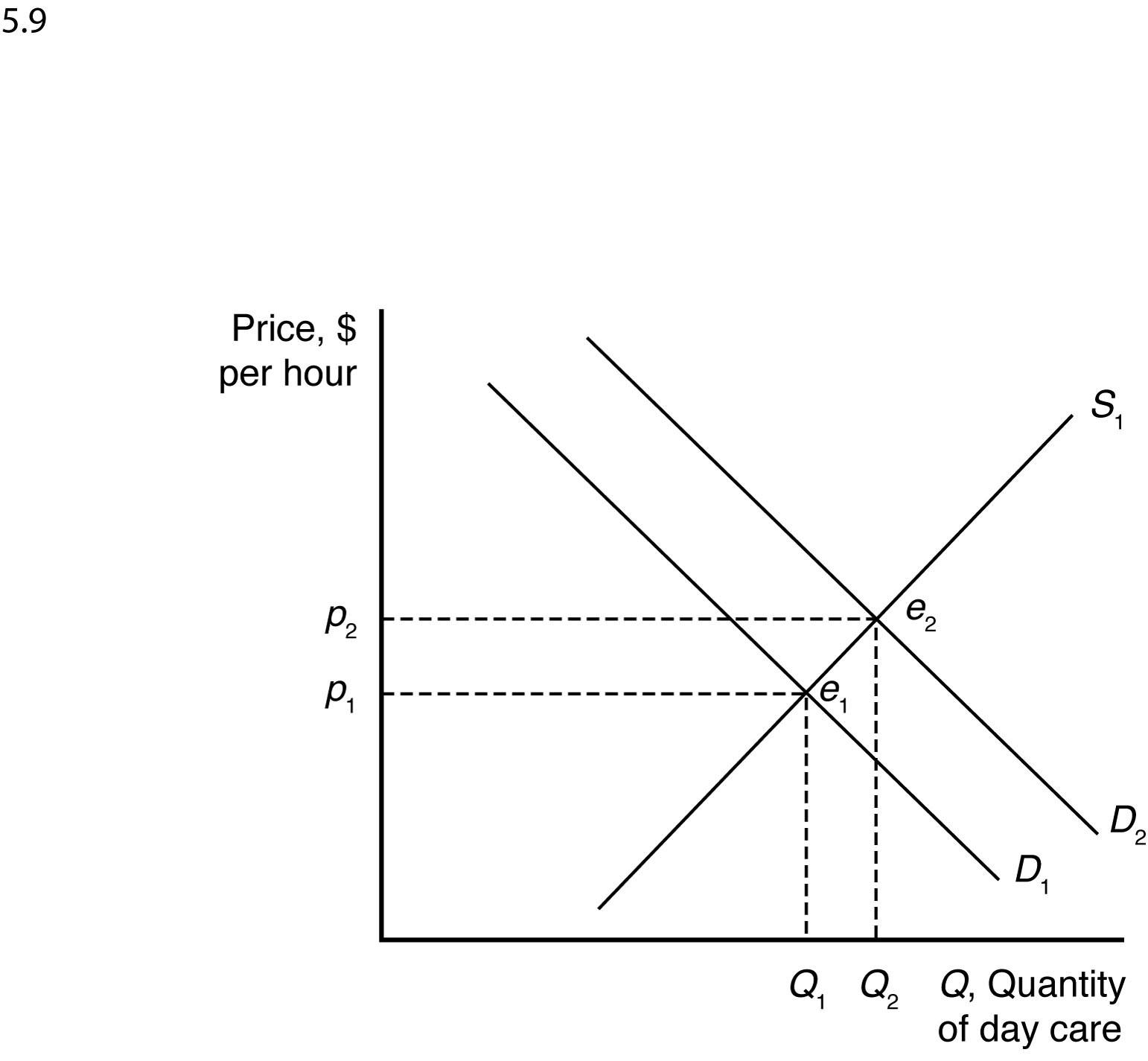
5.9 A daycare subsidy shifts the demand curve for daycare up by an amount equal to the size of the subsidy. The new equilibrium is where the new demand curve for daycare intersects the supply curve for daycare. This is at a higher equilibrium price and a higher equilibrium
6.1 The supply-and-demand model is accurate in perfectly competitive markets, which are markets in which all firms and consumers are price takers: no market participant can affect the market price. If there is only one seller of a good or service—a monopoly—that seller is a price taker and can affect the market price. Firms are also price setters in an oligopoly —a market with only a small number of firms. Experience has shown that the supply-anddemand model is reliable in a wide range of markets, such as those for agriculture, financial products, labor, construction, many services, real estate, wholesale trade, and retail trade.
7.1 A tax paid by consumers shifts the demand curve down by an amount equal to the size of the tax. Just the opposite, suspending a tax on consumers should raise the demand curve by an amount equal to the size of the suspended tax. Although fuel supply is more likely to be vertical in the short run than in the long run, equilibrium fuel prices will increase when the demand curve shifts up whether the supply curve is vertical or upward sloping.
©2014 Pearson Education, Inc.