If you want to buy this or Any Other Test Bank or Solution Manual contact us At.
Chapter 2
Supply and Demand
SOLUTIONS TO END-OF-CHAPTER QUESTIONS
DEMAND
1.1 When the price of coffee changes, the change in the quantity demanded reflects a movement along the demand curve. When other variables that affect demand change, the entire demand curve shifts. For example, when income changes, this causes coffee demand to shift.

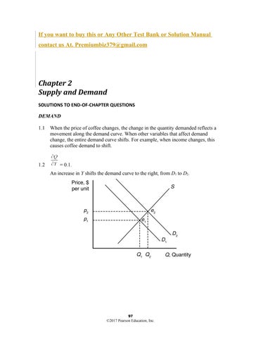
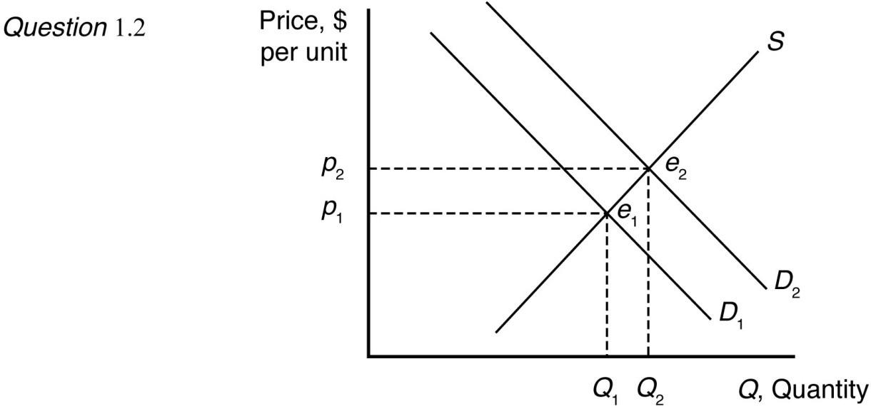
1.2 = 0.1.
An increase in Y shifts the demand curve to the right, from D1 to D2.
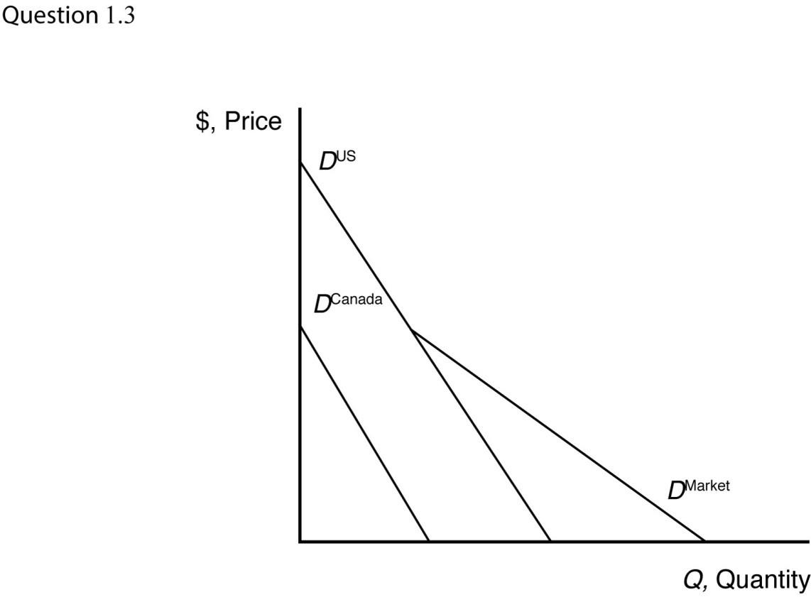
1.3 The market demand curve is the sum of the quantity demanded by individual consumers at a given price. Graphically, the market demand curve is the horizontal sum of individual demand curves.
1.4 a. The inverse demand curve for other town residents is p = 200 – 0.5Qr b. At a price of $300, college students demand 100 units of firewood, and other residents demand no firewood. Other residents will demand zero units of firewood
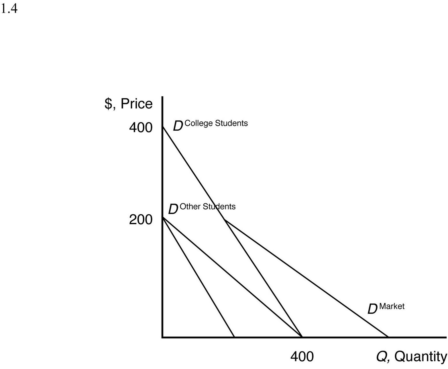
The market demand curve is the horizontal sum of individual demand curves, as
SUPPLY
2.1 The effect of a change in pf on Q is = –20pf = –20(1.10) = –22 units.

Thus, an increase in the price of fertilizer will shift the avocado supply curve to the left by 22 units at every price (i.e., a parallel shift to the left).
2.2 When the price of avocados changes, the change in the quantity supplied reflects a movement along the supply curve. When costs or other variables that affect supply change, the entire supply curve shifts. For example, the price of fertilizer represents a key factor of avocado production, which affects the cost of avocado production, shifting the avocado supply curve. This is because avocado prices are measured on a graph axis. Other factors that affect supply are not measured by a graph axis.
2.3 Given the supply function, Q = 58 + 15p – 20pf,
The effect of a change in p on Q is = 15p.

To change quantity by 60, price would need to change by 60 = 15p p = $4.00.
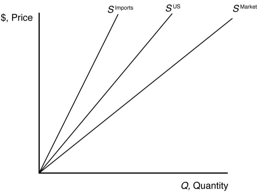
2.4 The market supply curve is the sum of the quantity supplied by individual producers at a given price. Graphically, the market supply curve is the horizontal sum of individual supply curves.
MARKET EQUILIBRIUM
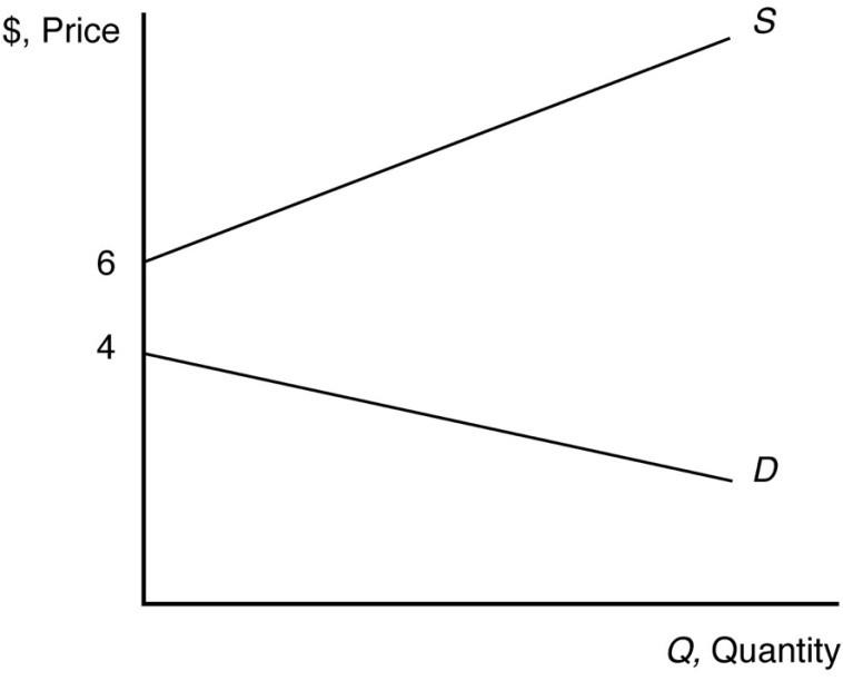
3.1 The supply curve is upward sloping and intersects the vertical price axis at $6. The demand curve is downward sloping and intersects the vertical price axis at $4. When all market participants are able to buy or sell as much as they want, we say that the market is in equilibrium: a situation in which no participant wants to change its behavior. Graphically, a market equilibrium occurs where supply equals demand. An equilibrium does not occur at a positive quantity because supply does not equal demand at any price.
3.2 The equilibrium price is p = 20 and the equilibrium quantity is Q = 80.
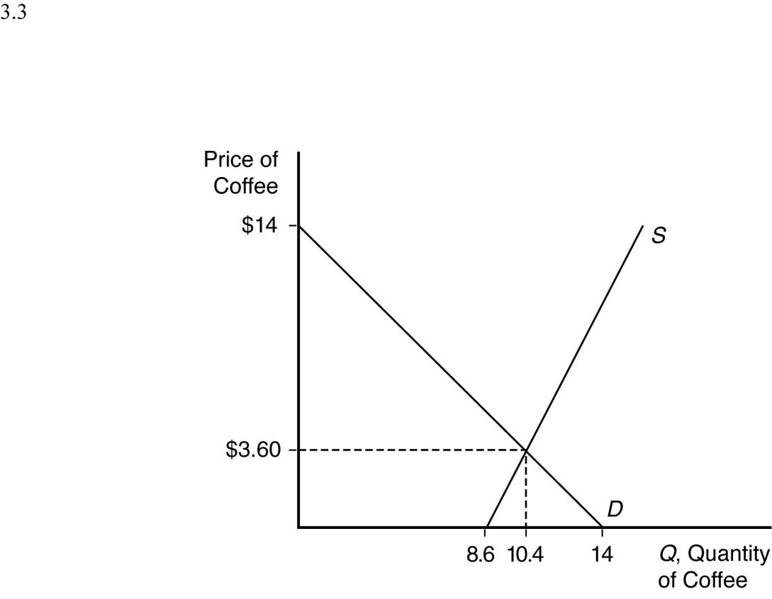
3.3 Given that pc = $5 and Y = $55,000 (note Y is measured in thousands, so the value to use here is 55), the demand for coffee can be rewritten as Q = 14 – p and the supply of coffee can be rewritten as Q = 8.6 + 0.5p
When all market participants are able to buy or sell as much as they want, we say that the market is in equilibrium: a situation in which no participant wants to change its behavior. Graphically, a market equilibrium occurs where supply equals demand. Thus, the equilibrium price is D = S
14 – p = 8.6 + 0.5p 5.4 = 1.5p p = $3.60.
Find the equilibrium quantity by substituting this price into either the supply or demand function. For example, using the supply function, the equilibrium quantity is
SHOCKS TO THE EQUILIBRIUM
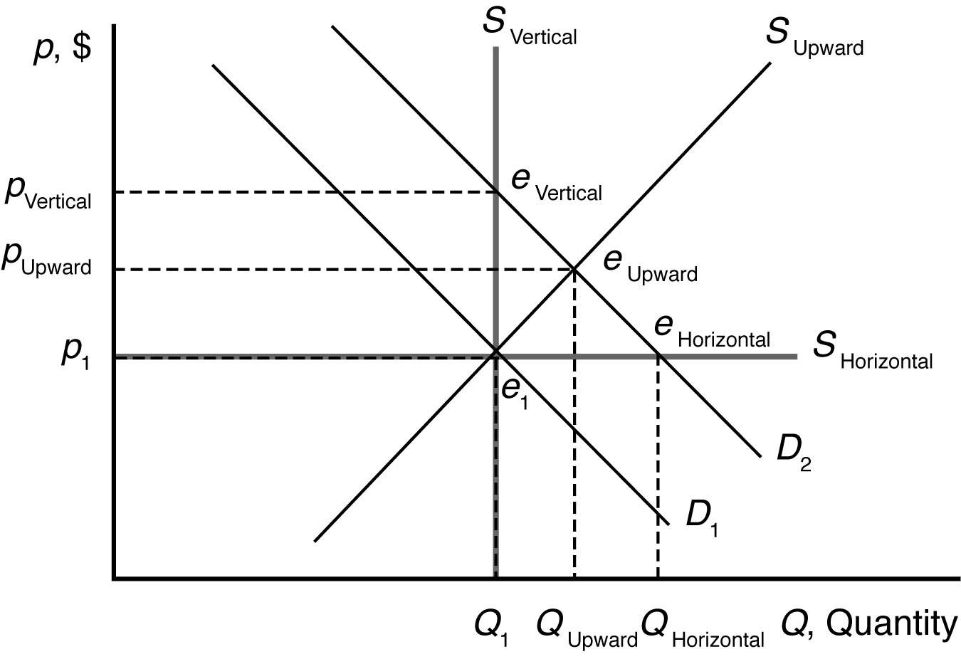
4.1 a. The new equilibrium with the horizontal supply curve is where the new demand curve intersects the horizontal supply curve. The new equilibrium price is unchanged. See figure.
b. The new equilibrium with the vertical supply curve is where the new demand curve intersects the vertical supply curve. The new equilibrium price is higher. See figure.
c. The new equilibrium with the upward-sloping supply curve is where the new demand curve intersects the upward-sloping supply curve. The new equilibrium price is higher. See figure.
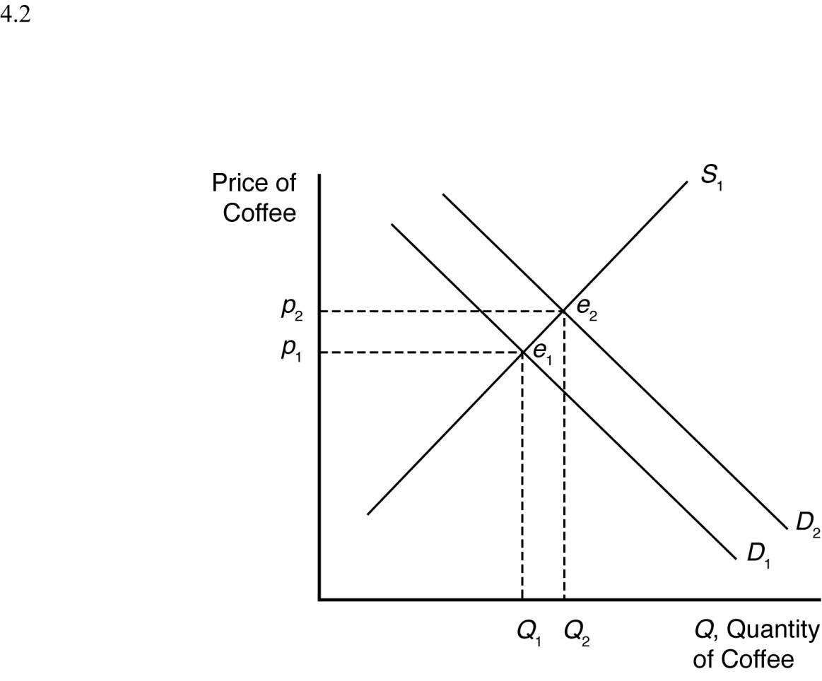
Health benefits from drinking coffee shift the demand curve for coffee to the right because more coffee is now demanded at each price. The new market equilibrium is where the original supply curve intersects the new coffee demand curve, at a
b. An increase in the usefulness of cocoa will increase demand for cocoa. This will drive up the equilibrium price of cocoa. Since cocoa and coffee are likely substitutes, this will increase the demand for coffee. The new market equilibrium is where the original supply curve intersects the new coffee
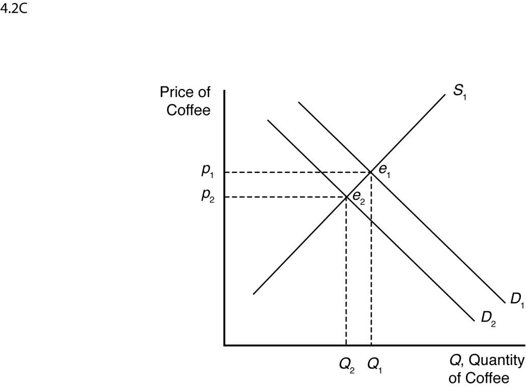
c. A recession shifts the demand curve for coffee to the left because less coffee is now demanded at each price. The new market equilibrium is where the original supply curve intersects the new coffee demand curve, at a lower price
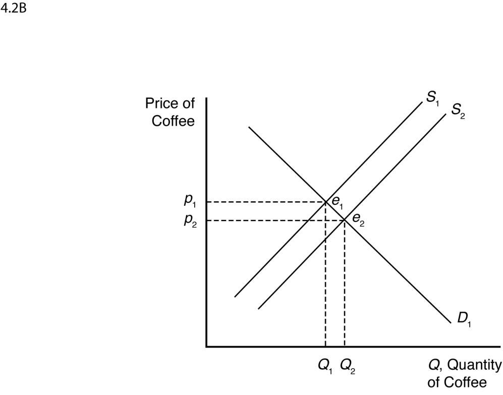
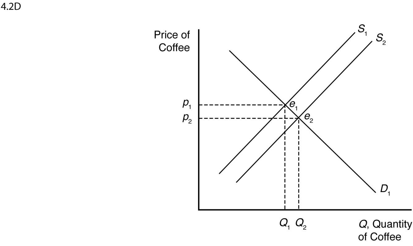
d. New technologies increasing yields shift the supply curve for coffee to the right because more coffee is now supplied at each price. The new market equilibrium is where the original demand curve intersects the new coffee
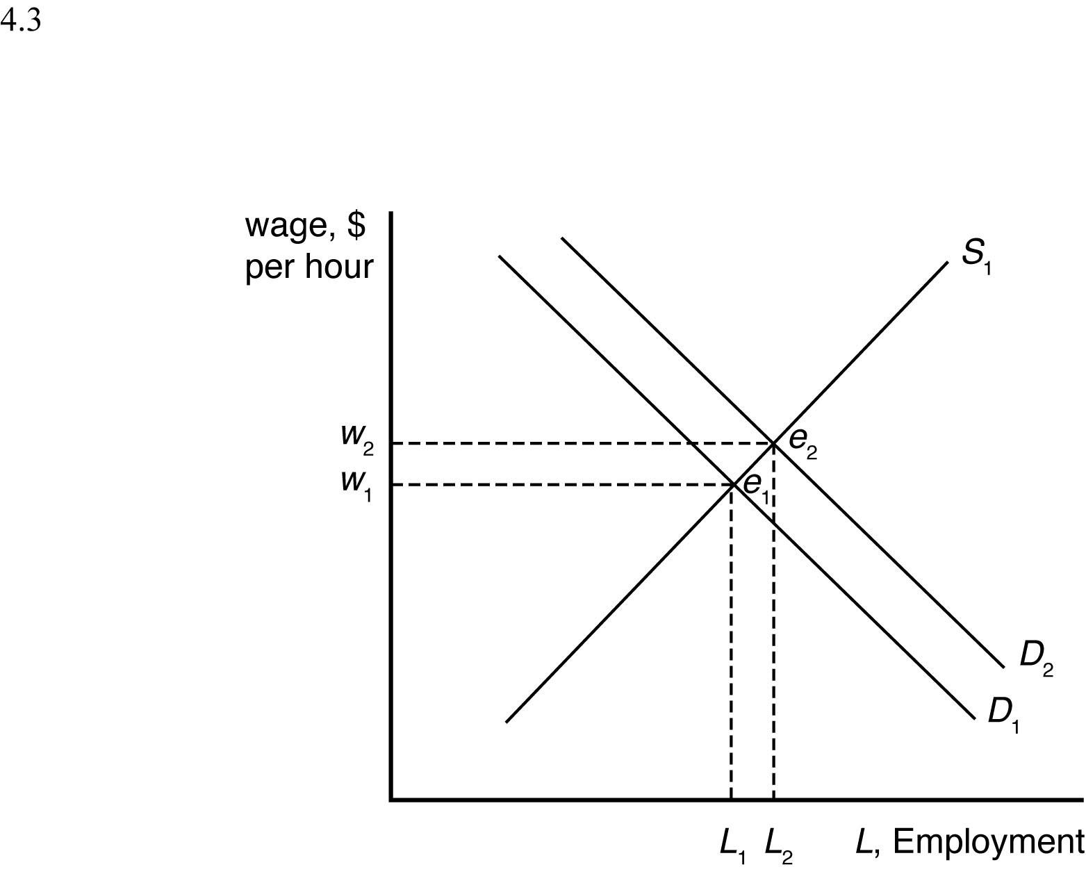
Outsourcing shifts the labor demand curve to the right because more Indian workers are demanded at each wage. The new market equilibrium is where the original
4.4 Given that pt = $0.80, the demand for avocados can be rewritten as Q = 160 – 40p and the supply of avocados can be rewritten as Q = 50 + 15p.
When all market participants are able to buy or sell as much as they want, we say that the market is in equilibrium: a situation in which no participant wants to change its behavior. Graphically, a market equilibrium occurs where supply equals demand. Thus, the equilibrium price is
D = S
160 – 40p = 50 + 15p 110 = 55p p = $2.00.
Find the equilibrium quantity by substituting this price into either the supply or demand function. For example, using the supply function, the equilibrium quantity is
Q = 50 + 15p
Q = 50 + 15(2.00)
Q = 50 + 30 Q = 80 units.
When the price of tomatoes increases to $1.35, the demand curve for avocados shifts out to
Q = 171 – 40p
The supply of avocados is unchanged. The new equilibrium is found where
D = S
171 – 40p = 50 + 15p
121 = 55p p = $2.20.
The equilibrium quantity is found as before
Q = 50 + 15p
Q = 50 + 15(2.20)
Q = 50 + 33
Q = 83 units.
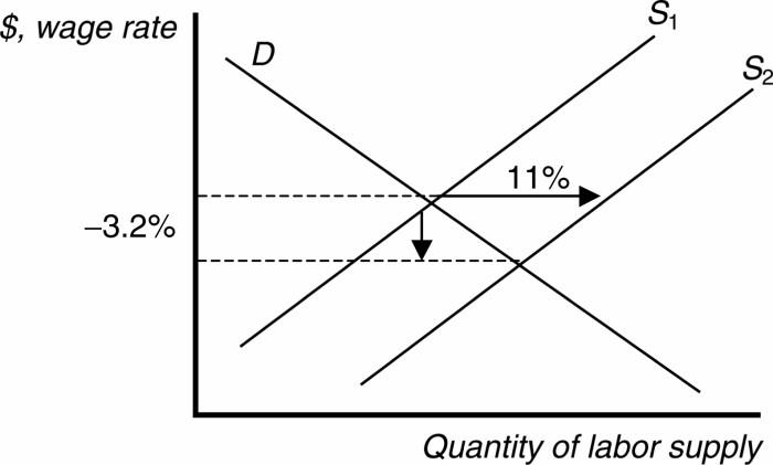
4.5 The numbers suggest that labor demand is inelastic. The supply curve shifts to the right by 11 percent, yet the decrease in equilibrium wage is only 3.2 percent.
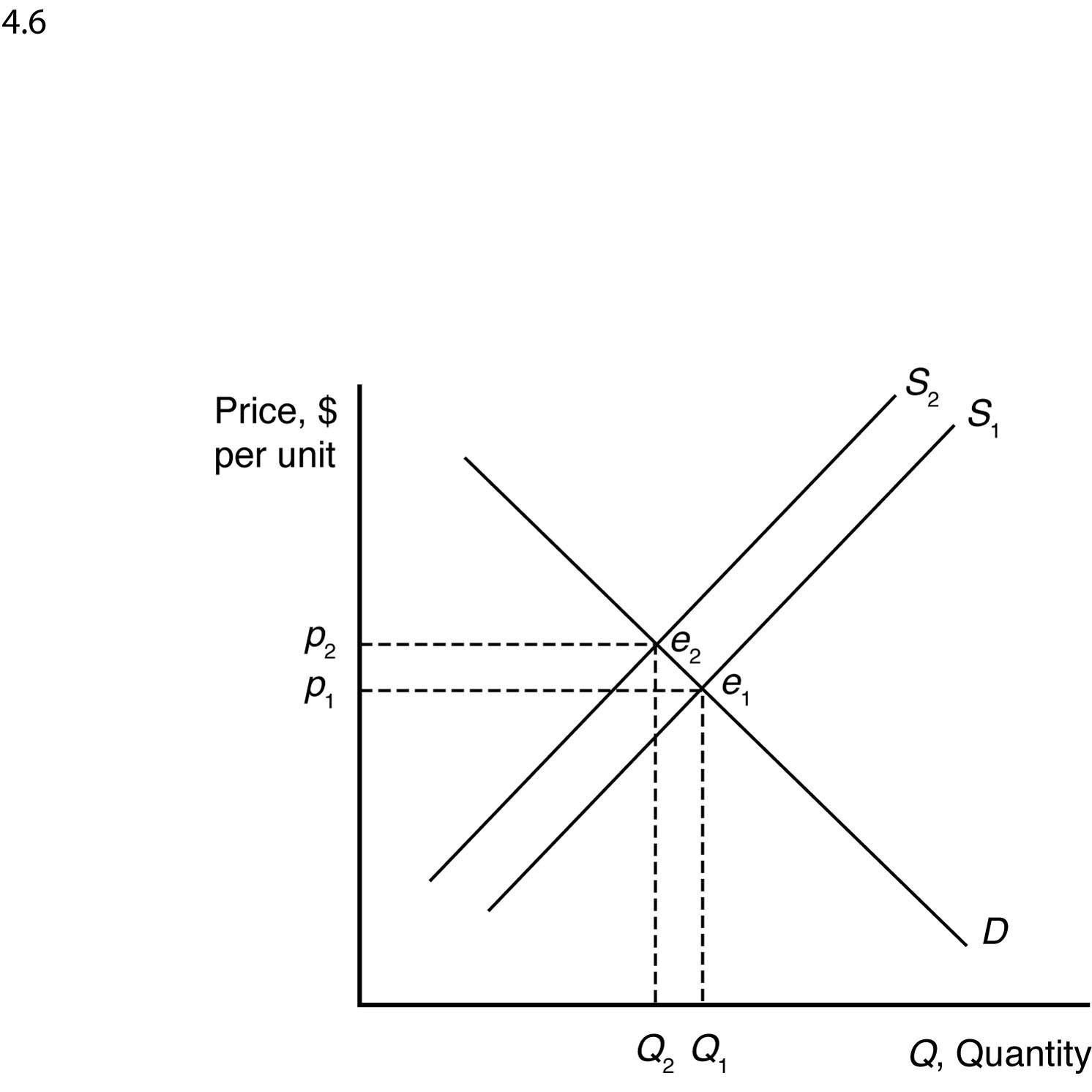
4.6 The damage reduces the supply of oranges, increasing the equilibrium price and
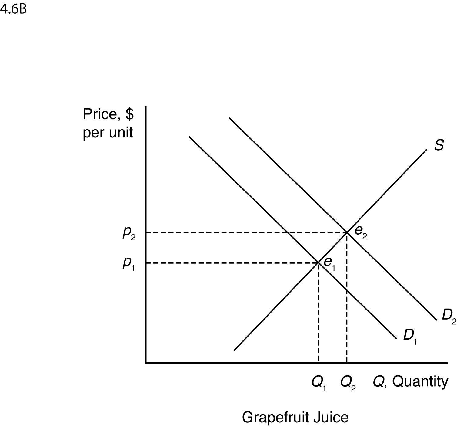
The demand for grapefruit juice increases as the price of orange juice increases because grapefruit juice is a substitute. As the demand for grapefruit juice increases,
4.7 The increased use of corn for producing ethanol will shift the demand curve for corn to the right. This increases the price of corn overall, reducing the consumption of corn as food.
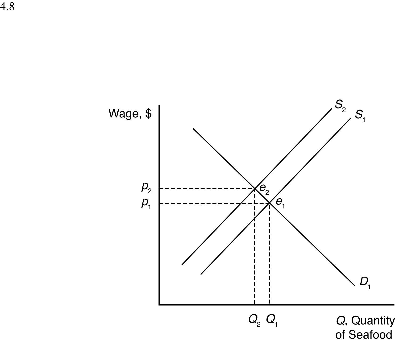
4.8 Suppose supply is initially S1, but it decreases by a small amount to S2 after the BP oil spill. When all market participants are able to buy or sell as much as they want, we say that the market is in equilibrium: a situation in which no participant wants to change its behavior. Graphically, a market equilibrium occurs where supply equals demand. The original market equilibrium is where the original demand curve ). The new market equilibrium is where the ). When the supply curve shifts by a relatively small amount, the change in the equilibrium price is likely to
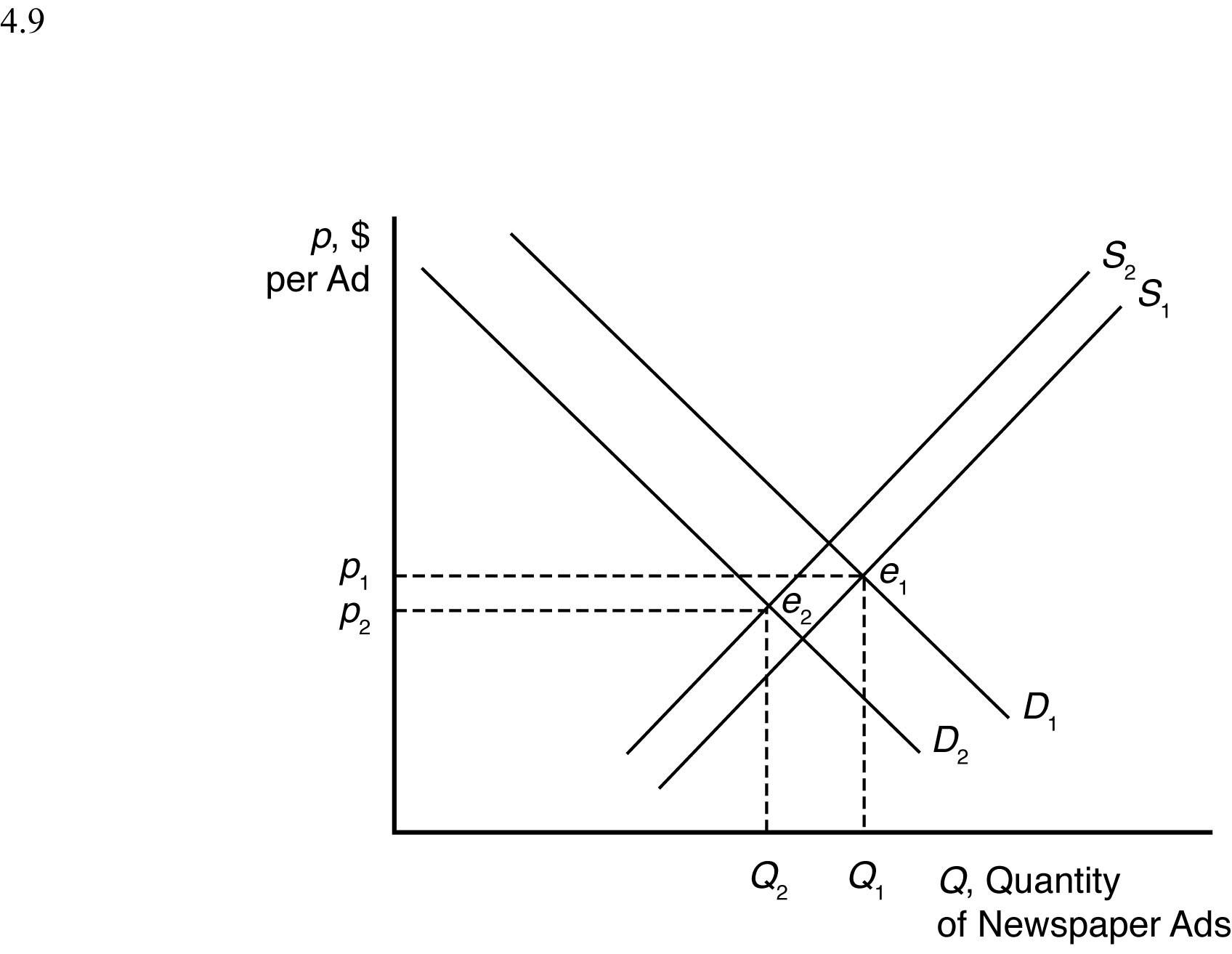
4.9 The Internet shifts the demand curve for newspaper advertising to the left because fewer companies demand newspaper advertising with online advertising available. The Internet may force some newspapers out of business, so the supply curve for newspaper advertising will shift to the left some. The new market equilibrium is where the new demand curve intersects the new supply curve. At the new
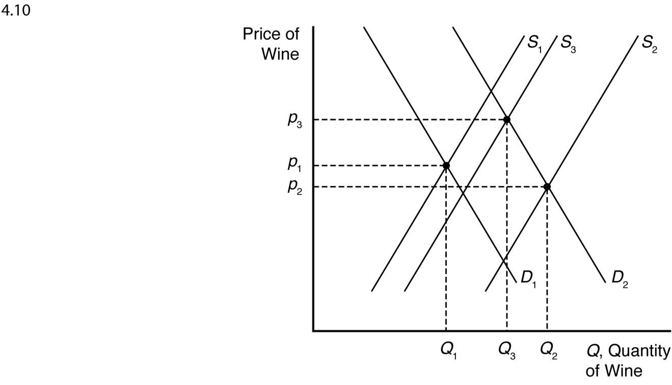
4.10 If global warming causes both an increase in the supply of wine during a period of time when the demand for wine is also rising, then the overall effect on the equilibrium quantity of wine will be for the quantity to increase. This is true because both the increase in supply (from S1 to S2 or S3) and the increase in demand (from D1 to D2) will result in higher equilibrium quantities on their own, and so the combination of the two effects will definitely be an increase in quantity. The effect of these events on the equilibrium price of wine, however, is indeterminate. The increase in demand will lead to a higher equilibrium price, but the increase in supply will lead to a lower equilibrium price. Taken together, the net effect on price will be determined by how large the shifts of supply and demand are relative to one another. If the supply shift is larger (from S1 to S2), then price will fall. If, on the other hand, the demand shift is larger, then price will rise.
4.11 An increase in petroleum prices shifts the aluminum supply curve to the left because the cost of producing aluminum is more expensive at each price. An increase in the cost of petroleum also shifts the demand curve for aluminum to the right because the petroleum price increase makes a substitute, plastic, more expensive (by making the cost of plastic production higher). The new equilibrium is where the new aluminum supply curve intersects the new aluminum demand curve.

When the supply curve shifts to the left, the new equilibrium price is higher, and the new equilibrium quantity is lower. When the demand curve shifts to the right, the new equilibrium price is higher, and the new equilibrium quantity is higher. When both curves shift, the new equilibrium price is higher, but the new equilibrium
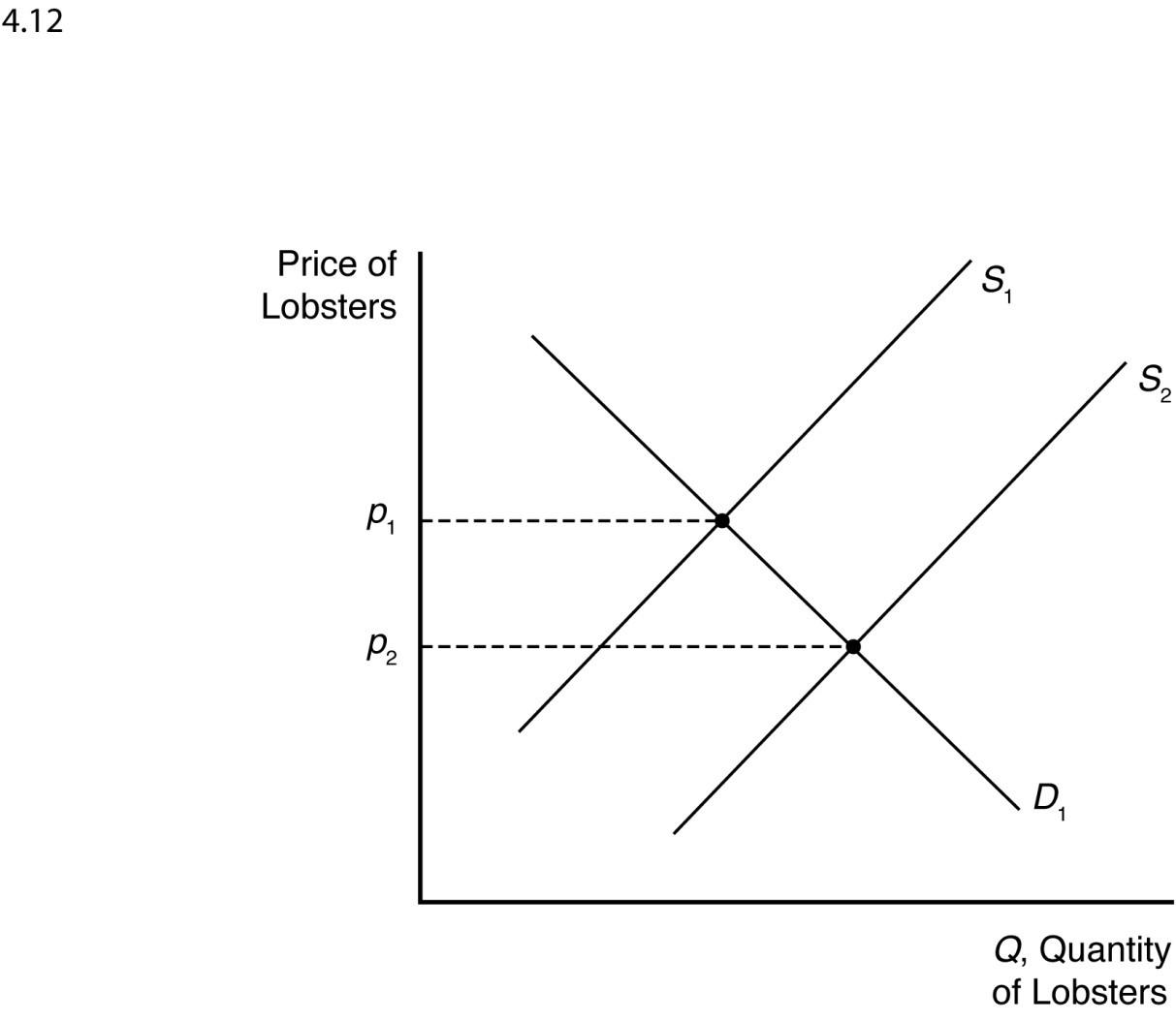
The cartoon seems to show a bumper harvest of lobsters. A large increase in the ), which will cause price
EFFECTS OF GOVERNMENT INTERVENTIONS
5.1 Requiring occupational licenses shifts the labor supply curve to the left because fewer people are able to supply their labor at each wage. The new market equilibrium is where the original demand curve intersects the new labor supply curve, at a higher wage and lower employment level.
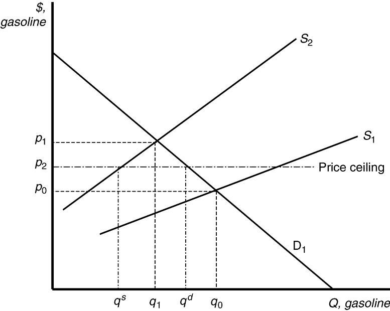
5.2 In the absence of price controls, the leftward shift of the supply curve as a result of Hurricane Katrina would push market prices up from p0 to p1 and reduce quantity from q0 to q1. At a government imposed maximum price of p2, consumers would want to purchase qd units, but producers would only be willing to sell qs units. The resulting shortage would impose search costs on consumers, making them worse off. The reduced quantity and price also reduce firms’ profits.
5.3 With a binding price ceiling, such as a ceiling on the rate that can be charged on loans, some consumers who demand loans at the rate ceiling will be unable to obtain them. This is because the demand for bank loans is greater than the supply of bank loans to low-income households with the usury law.
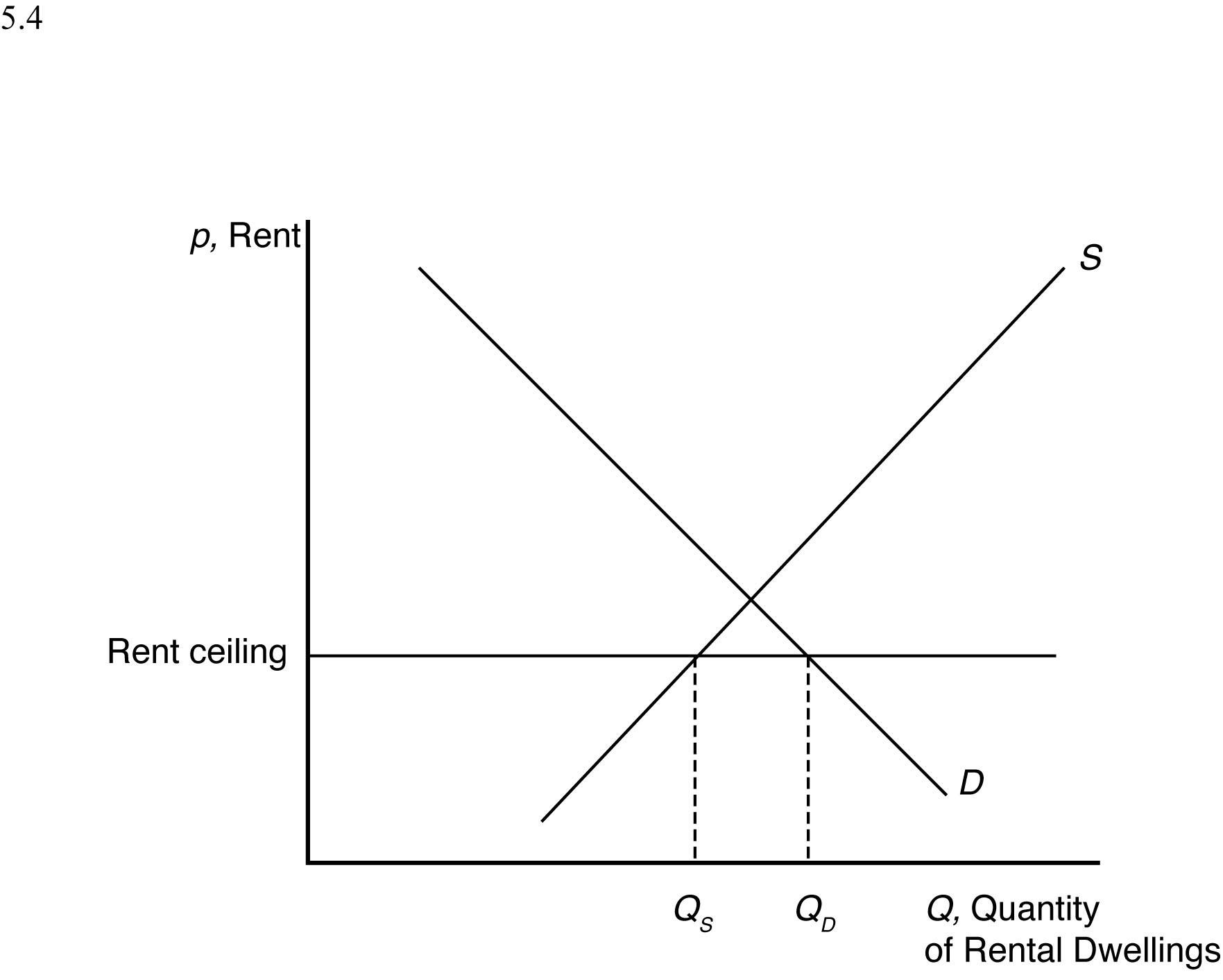
5.4 With the binding rent ceiling, the quantity of rental dwellings demanded is that ). The quantity of rental dwellings supplied is that quantity where the rent ceiling intersects the supply ). With the rent control laws, the quantity supplied is less than the quantity
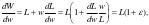
5.5 We can determine how the total wage payment, W = wL(w), varies with respect to w by differentiating. We then use algebra to express this result in terms of an elasticity: where is the elasticity of demand of labor. The sign of dW/dw is the same as that of 1 + . Thus total labor payment decreases as the minimum wage forces up the wage if labor demand is elastic, <–1, and increases if labor demand is inelastic, >–1.
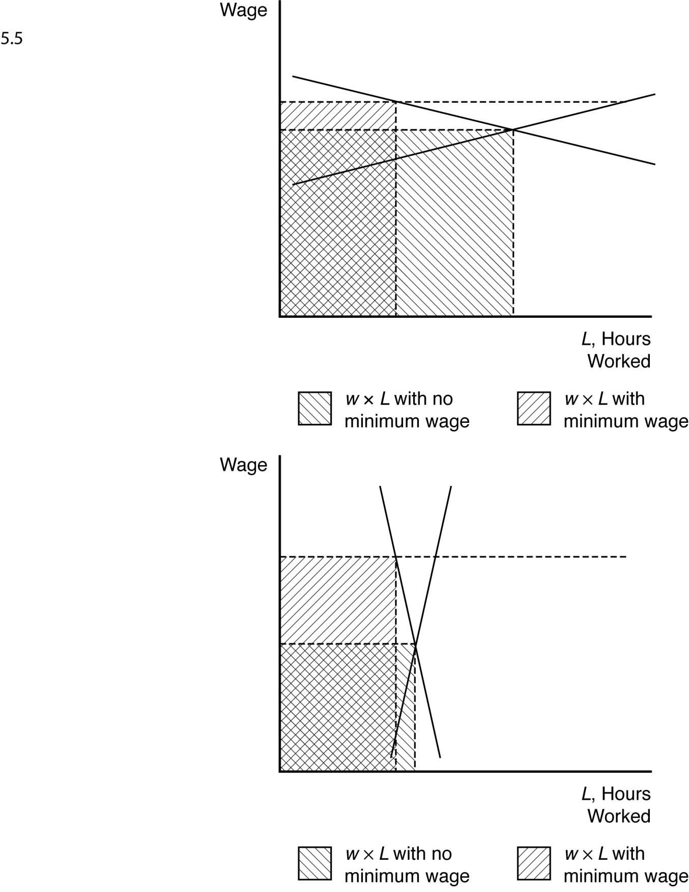
For a graphical explanation, see the figures below. In the top panel with very flat supply and demand curves, the imposition of a minimum wage causes overall wage payments to fall dramatically. On the other hand, when supply and demand curves are steep (as in the bottom panel) overall wage payments increase substantially.
5.6 Before the tax is imposed, the demand for avocados can be rewritten as
Q = 160 – 40p and the supply of avocados is given as
Q = 50 + 15p
When all market participants are able to buy or sell as much as they want, we say that the market is in equilibrium: a situation in which no participant wants to change its behavior. Graphically, a market equilibrium occurs where supply equals demand. Thus, the equilibrium price is
D = S
160 – 40p = 50 + 15p 110 = 55p p = $2.00.
Find the equilibrium quantity by substituting this price into either the supply or demand function. For example, using the supply function, the equilibrium quantity is
Q = 50 + 15p
Q = 50 + 15(2.0)
Q = 50 + 30
Q = 80 units.
If a $0.55 tax is imposed, the demand curve can be rewritten to account for the tax. First, the demand curve can be rewritten as inverse demand by solving for p
Q = 160 – 40p p = 4 – 0.025Q.
The tax is subtracted from inverse demand to give p = 3.45 – 0.025Q and then this inverse demand curve can be turned back into a demand curve
Q = 138 – 40p.
Setting supply equal to demand, the new equilibrium (pretax) price is
D = S
138 – 40p = 50 + 15p 88 = 55p p = $1.60.
The after-tax price is $2.15.
Using the supply function, the equilibrium quantity is
Q = 50 + 15p
Q = 50 + 15(1.60)
Q = 50 + 24
Q = 74 units.
5.7 A tax on consumers will shift the demand curve down by an amount equal to the size of the tax. The new equilibrium price and quantity with the tax will be where the new demand curve intersects the original supply curve. The decrease in quantity will be larger the more horizontal the supply curve is. Just the opposite, the equilibrium quantity will not decrease at all if the supply curve is completely vertical.
5.8 a. If demand is vertical and supply is upward sloping, then all the tax burden is paid by consumers because they are not price sensitive.
b. If demand is horizontal and supply is upward sloping, then all the tax burden is paid by producers because consumers are infinitely price sensitive.
c. If demand is downward sloping and supply is horizontal, then all the tax burden is paid by consumers because producers are infinitely price sensitive.
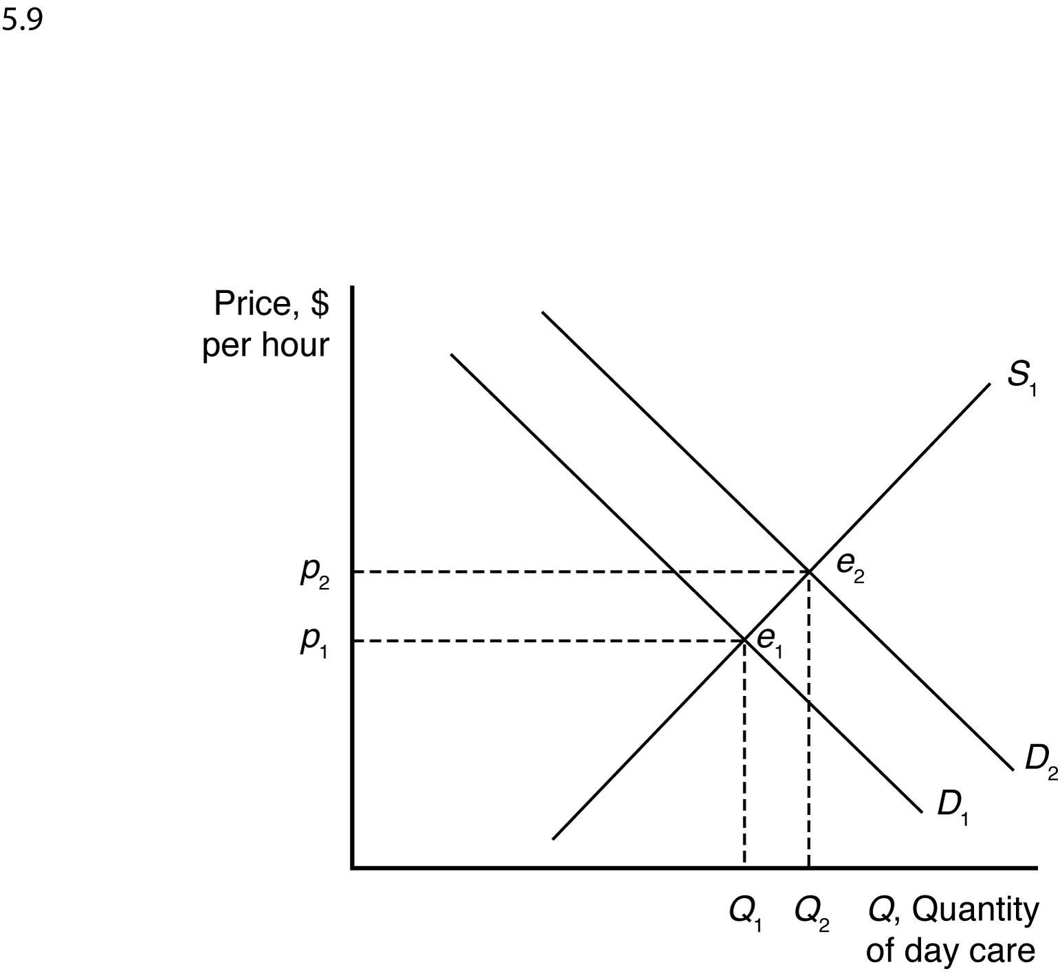
5.9 A daycare subsidy shifts the demand curve for daycare up by an amount equal to the size of the subsidy. The new equilibrium is where the new demand curve for daycare intersects the supply curve for daycare. This is at a higher equilibrium
WHEN TO USE THE SUPPLY-AND-DEMAND MODEL
6.1 The supply-and-demand model is accurate in perfectly competitive markets, which are markets in which all firms and consumers are price takers: no market participant can affect the market price. If there is only one seller of a good or service—a monopoly—that seller is a price taker and can affect the market price. Firms are also price setters in an oligopoly—a market with only a small number of firms. Experience has shown that the supply-and-demand model is reliable in a wide range of markets, such as those for agriculture, financial products, labor, construction, many services, real estate, wholesale trade, and retail trade.
MANAGERIAL PROBLEM
7.1 A tax paid by consumers shifts the demand curve down by an amount equal to the size of the tax. Just the opposite, suspending a tax on consumers should raise the demand curve by an amount equal to the size of the suspended tax. Although fuel supply is more likely to be vertical in the short run than in the long run, equilibrium fuel prices will increase when the demand curve shifts up whether the supply curve is vertical or upward sloping.
SOLUTIONS TO SPREADSHEET EXERCISES
See the associated Excel files.