Issuu

Engineering Vibration 4th

Full chapter download at: https://testbankbell.com/product/solutions-manual-for-engineering-vibration4th-by-inman-0132871696/

Problems and Solutions Section 1.4 (problems 1.65 through 1.81)

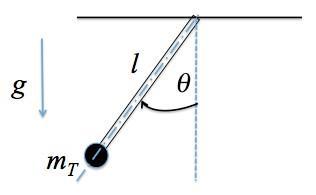
1.65 Calculate the frequency of the compound pendulum of Figure P1.65 if a mass mT is added to the tip, by using the energy method. Assume the mass of the pendulum is evenly distributed so that its center of gravity is in the middle of the pendulum of length l.

Solution Adding a tip mass adds both kinetic and potential energy to the system. If the mass of the pendulum bar is m, and it is lumped at the center of mass the energies become:

Conservation of energy (Equation 1.51) requires T + U = constant:

Differentiating with respect to time yields:

Rearranging and approximating using the small angle formula sin θ ~ θ, yields:

Figure P1.65 A compound pendulum with a tip mass.

U = 1(  cosθ)mg + (  cosθ)m g Potential Energy: 2 =  (1 cosθ)(mg + 2m g) 2 t T = 1 Jθ 2 + 1 J θ 2 = 1 m θ 2 + 1 m 2θ 2 Kinetic Energy: 2 2 t 2 3 2 t = ( 1 m + 1 m )2θ 2 6 2 t

 (1 cosθ)(mg + 2m g) + ( 1 m + 1 m )2θ ˙2 = C 2 t 6 2 t

 (sinθ)(mg + 2m g)θ  + ( 1 m + m )2θ  θ  = 0 2 t 3 t 1 1 ⇒ ( m + mt )θ  + 3 2(mg + 2mt g)sinθ = 0

Note that this solution makes sense because if mt = 0 it reduces to the frequency of the pendulum equation for a bar, and if m = 0 it reduces to the frequency of a massless pendulum with only a tip mass.

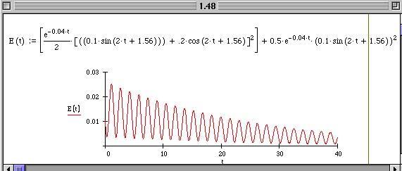
1.66 Calculate the total energy in a damped system with frequency 2 rad/s and damping ratio ζ = 0.01 with mass 10 kg for the case x0 = 0.1 m and v0 = 0. Plot the total energy versus time.

Solution: Given: ωn = 2 rad/s,

Calculate the stiffness and damped natural frequency:

The total energy of the damped system is

Applying the initial conditions to evaluate the constants of integration yields:

ζ = 0.01, m = 10 kg, x0 = 0.1 m, v0 = 0.

k = mω 2 = 10(2)2 2 = 40 N/m 2 ωd = ω n 1 ζ = 2 1 0.01 = 2 rad/s

1 1 where E(t) = x(t) = Ae 0 02 t sin(2t + φ) mx ˙2 (t) + 2 kx(t) 2 x ˙(t) = 0.02 Ae 0 02 t sin(2t + φ) + 2Ae 0.02t cos(2t + φ)

x(0) = 0.1 = Asinφ x(0) = 0 = 0.02Asinφ + 2Acosφ ⇒φ = 1.57 rad, A = 0.1 m Substitution

E(t)

of these values into

yields:

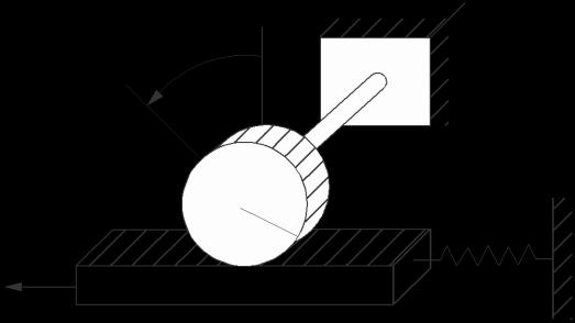
1.67 Use the energy method to calculate the equation of motion and natural frequency of an airplane's steering mechanism for the nose wheel of its landing gear. The mechanism is modeled as the single-degree-of-freedom system illustrated in Figure P1.54. (Steering wheel)

The steering wheel and tire assembly are modeled as being fixed at ground for this calculation. The steering rod gear system is modeled as a linear spring and mass system (m, k2) oscillating in the x direction. The shaft-gear mechanism is modeled as the disk of inertia J and torsional stiffness k2. The gear J turns through the angle θ such that the disk does not slip on the mass. Obtain an equation in the linear motion x

J k1 r (Tire–wheel k2 assembly) x m

Solution: From kinematics: x = rθ,⇒ x ˙ = rθ ˙ Kinetic energy: T = 1 Jθ 2 + 1 mx 2 Potential energy: 2 U = 1 k 2 x 2 + 1 k θ 2 2 2 2 1 Substitute θ = x :T + U = 1 J x  2 + 1 mx  2 + 1 k x 2 + 1 k1 x 2 r Derivative: J 2 r 2 2 2 2 d(T +U )= 0 dt k1 2 r 2 x  x  + mx  x  + k xx  + xx  = 0 r 2 2 r 2 ⎡⎛ J ⎞ ⎛ k1 ⎞ ⎤ ⎣ ⎢⎝ r 2 + m⎠ x  + ⎝ k2 + r 2 ⎠ x x  = 0 Equation of motion: ⎛ J + m ⎞˙ x ˙ + ⎛k k + x = 0 ⎝ r 2 ⎠ ⎝ 2 r 2 ⎠ kk + 1 2 Natural frequency: ω n = 2 r 2 = J + m k + r k J + mr 2

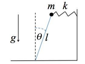
1.68 Consider the pendulum and spring system of Figure P1.68. Here the mass of the pendulum rod is negligible. Derive the equation of motion using the energy method. Then linearize the system for small angles and determine the natural frequency. The length of the pendulum is l, the tip mass is m, and the spring stiffness is k

Figure P1.68 A simple pendulum connected to a spring

Solution: Writing down the kinetic and potential energy yields:

Here the soring deflects a distance lsinθ, and the mass drops a distance l(1 –cosθ).

Adding up the total energy and taking its time derivative yields:

1.69 A control pedal of an aircraft can be modeled as the single-degree-of-freedom system of Figure P1.69. Consider the lever as a massless shaft and the pedal as a lumped mass at the end of the shaft. Use the energy method to determine the

07458. n

Upper Saddle River, NJ

T = 1 ml2θ 2 , U = 1 kx2 + mgh 2 2 U = 1 kl2 sin2θ + mgl(1 cosθ) 2

d ⎛ 1 ml2θ 2 + 1 kl2 sin2θ + mgl cosθ⎞ dt ⎝ 2 2 ⎠ = (ml2θ)θ + (kl2 sinθcosθ)θ mgl sinθθ = 0 ⇒ ml2θ  + kl2 sinθcosθ mgl sinθ = 0 For small θ, this becomes ml2θ + kl2θ mglθ = 0 ⇒θ  + kl mgθ = 0 ml ⇒ω = kl mg rad/s ml

equation of motion in θ and calculate the natural frequency of the system. Assume the spring to be unstretched at θ = 0.

Solution: In the figure let the mass at θ = 0 be the lowest point for potential energy. Then, the height of the mass m is (1-cos

k l1 l2 m

Figure P1.69

θ)2. Kinematic relation: x = 1θ Kinetic Energy: T = 1 mx ˙2 = 2 1 m2θ ˙2 2 Potential Energy: U = 1 2 2 k(1θ) + mg2(1 cosθ) Taking the derivative of the total energy yields: d (T + U) = m2θ ˙ θ ˙˙ + k( 2θ)θ ˙ + mg (sinθ)θ = 0 dt 2 1 2 Rearranging, dividing by dθ/dt and approximating sinθ with θ yields: 2˙˙ 2 m2θ + (k1 + mg2 )θ = 0 ⇒ ω n = k2 + mg m2

1.70 To save space, two large pipes are shipped one stacked inside the other as indicated in Figure P1.70. Calculate the natural frequency of vibration of the smaller pipe (of radius R1) rolling back and forth inside the larger pipe (of radius R). Use the energy method and assume that the inside pipe rolls without slipping and has a mass m

Solution: Let θ be the angle that the line between the centers of the large pipe and the small pipe make with the vertical and let α be the angle that the small pipe rotates through. Let R be the radius of the large pipe and R1 the radius of the smaller pipe. Then the kinetic energy of the system is the translational plus rotational of the small pipe. The potential energy is that of the rise in height of the center of mass of the small pipe.

From the drawing: y + (R R1)cosθ + R1 = R

⇒ y = (R R1)(1 cosθ) ⇒ y ˙ = (R R1)sin(θ)θ ˙

Likewise examination of the value of x yields: x = (R R1)sinθ

⇒ x ˙ = (R R1)cosθθ ˙

Let β denote the angle of rotation that the small pipe experiences as viewed in the

Large pipe Small pipe a' O' R O b R1 a Truck bed (a) mg (b)

Figure P1.70

R θ R –

1 y R

1 x

inertial frame of reference (taken to be the truck bed in this case). Then the total kinetic energy can be written as:

The total potential energy becomes just:

Now it remains to evaluate the angle β. Let α be the angle that the small pipe rotates in the frame of the big pipe as it rolls (say) up the inside of the larger pipe. Then

were α is the angle “rolled” out as the small pipe rolls from a to b in figure P1.56. The rolling with out slipping condition implies that arc length a’b must equal arc length ab. Using the arc length relation this yields that Rθ =R1α.

Substitution of the expression β = θ–α yields:

which is the relationship between angular motion of the small pipe relative to the ground (β) and the position of the pipe (θ). Substitution of this last expression into the kinetic energy term yields:

T = Ttrans + Trot = 1 1 mx ˙2 + 2 2 2 1 my ˙2 + 2 2 I0β ˙ 2 2 1 ˙ 2 = 2 m(R R1 ) (sin θ + cos θ)θ ˙ + 2 I0β ⇒ T = 1 2 m(R R1)2 θ ˙2 + 1 I β ˙ 2 2

= mgy =

mg(R R1)(1 cos

)

β = θ–

Rθ = R1(θ β) = R1θ R1β⇒ (R R1 )θ = R1β ⇒ β = 1 (R1 R)θ and 1 β ˙ = (R1 R)θ ˙ R1

1 T = 2 m(R R1)2θ ˙2 1 + 2 I0( 1 R1 (R1 R)θ ˙ ) ⇒ T = m(R R1)2θ2 Taking the derivative of T + V yields d dθ (T + V)= 2m(R R )2θ ˙ θ ˙˙ + mg(R R )sinθθ ˙ =0 1 1 ⇒ 2m(R R )2θ ˙˙ + mg(R R )sinθ =0 Using the small angle approximation for sine this becomes 2m(R R )2θ + mg(R R )θ = 0 ⇒ θ ˙˙ + g θ = 0 2(R R1) ⇒ ω n = g 2(R R1 )

1.71 Consider the example of a simple pendulum given in Example 1.4.2. The pendulum motion is observedto decaywith a dampingratio ofζ =0.001.Determine a damping coefficient and add a viscous damping term to the pendulum equation.

Solution: From example 1.4.2, the equation of motion for a simple pendulum is

g . With viscous damping the equation of motion in normalized form

θ +

0 

g θ =

So ω n = becomes:  θ ˙˙ +2ζω θ ˙ +ω 2θ = 0 or with ζ as given : n n ⇒ θ +2(.001)ω n θ +ω n θ = 0 The coefficient of the velocity term is c c = J m2 =(.002) g  c =(0.002)m g3

1.72 Determine a damping coefficient for the disk-rod system of Example 1.4.3. Assuming that the damping is due to the material properties of the rod, determine c for the rod if it is observed to have a damping ratio of ζ = 0.01.

Solution: The equation of motion for a disc/rod in torsional vibration is

1.73 The rod and disk of Window 1.1 are in torsional vibration. Calculate the damped natural frequency if J

Jθ  + kθ = 0 or Add viscous damping: θ  + ω 2θ = 0 where ω = k J θ  + 2ζω n θ  +ω n θ = 0 θ + 2(.01) kθ +ω 2θ = 0 J n

coefficient

be c = (0.02) k ⇒ c = 0.02 kJ

From the velocity term, the damping

must

m2 ⋅ kg, c = 20 N⋅ m⋅ s/rad, and k = 400 N⋅m/rad. Solution:

Jθ  + cθ  + kθ = 0 The damped natural frequency is ω d = ω n 1 ζ where ω n = k 400 = = 0.632 rad/s J 1000 and ζ = c = 20 = 0.0158 2 kJ 2 400×1000 Thus the damped natural frequency is ω d = 0.632 rad/s

= 1000

The equation of motion is

1.74 Consider the system of P1.74, which represents a simple model of an aircraft landing system. Assume, x = rθ. What is the damped natural frequency?

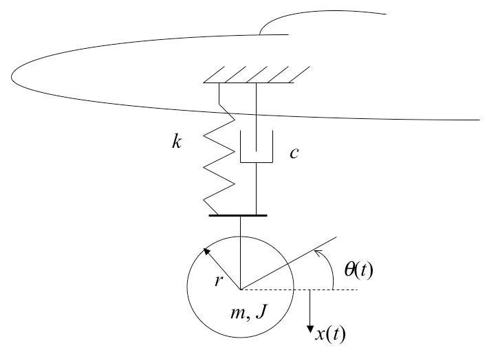
Solution: Ignoring the damping and using the energy method the equation of motion is

Thus the undamped equation of motion is:

From examining the equation of motion the natural frequency is:

An add hoc way do to this is to add the damping force to get the damped equation of motion:

The value of ζ is determined by examining the velocity term:

Figure P1.74

T = 1 Jθ 2 + 1 mx 2 , U = 1 kx2 , θ = x 2 2 2 r 2 d (T +U)= d ⎛ 1 J x 1 1 ⎞ + mx 2 + kx2 dt dt 2 r 2 2 2 J ⇒ r 2 xx + mxx + kxx

⎛ m J ⎞ ⎝ r 2 ⎠˙ x ˙ + kx = 0

ω n = k k = m eq m + r 2

⎛ m J ⎞ ⎝ r 2 ⎠˙ x ˙ + cx ˙ + kx = 0

Thus the damped natural frequency is

1.75 Consider Problem 1.74 with k = 400,000 N/m,

= 1500 kg,

= 100

kg/rad, r = 25 cm, and c = 8000 kg/s. Calculate the damping ratio and the damped natural frequency. How much effect does the rotational inertia have on the undamped natural frequency?

Solution: From problem 1.74:

2 ⎛ ⎞ 2 k ⎜ c ⎟ ω d = ω n 1 ζ = m + J 1 ⎜ ⎜ ⎟ ⎛ J ⎞⎟ 2 2 k m + ⎝ r 2 ⎠ ⇒ω d = k m + J ⎛ c 2 2 = J ⎞ r 2(mr 2 + J) 4(kmr2 + kJ) c 2 r 2 r 2 4 m + r 2

m2 ⋅

ζ = c and ω k c 2 = 2 k⎛ m + J ⎞ m + J ⎛ J ⎞ 2 Given: ⎝ r 2 ⎠ r 2 k = 4×105 N/m m = 1.5×103 kg J = 100 m 2kg/rad r = 0.25 m and c = 8×103 N⋅s/m

Inserting the given values yields

ζ = 0.114 and ω d = 11.29 rad/s

For the undamped natural frequency, ω n =

With the rotational inertia, ω n = 11.36 rad/s

Without rotational inertia, ω n = 16.33 rad/s

The effect of the rotational inertia is that it lowers the natural frequency by almost 33%.

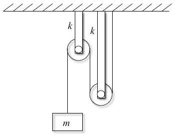
1.76 Use Lagrange’s formulation to calculate the equation of motion and the natural frequency of the system of Figure P1.76. Model each of the brackets as a spring of stiffness k, and assume the inertia of the pulleys is negligible.

Solution: Let x denote the distance mass m moves, then each spring will deflects a distance x/4. Thus the potential energy of the springs is

The kinetic energy of the mass is

Using the Lagrange formulation in the form of Equation (1.64):

k m + J / r 2

Figure P1.76

2 U = 2×

1 ⎛ x⎞ 2 k ⎝ ⎜ 4⎠ ⎟ = k x 2 16 T = 1 2 mx 2

2 d ⎛ ∂ ⎛ 1 2 ⎞⎞ mx  ∂ ⎛ kx ⎞ d k ⎜ ⎟ + ⎜ ⎟ = 0 ⇒ (mx )+ x = 0 dt ⎝∂x 2 ⎠ ∂x ⎝ 16 ⎠ ⇒ mx + dt 8 k 1 x = 0 ⇒ω n = k rad/s

1.77 Use Lagrange’s formulation to calculate the equation of motion and the natural frequency of the system of Figure P1.77. This figure represents a simplified model of a jet engine mounted to a wing through a mechanism which acts as a spring of stiffness k and mass ms. Assume the engine has inertia J and mass m and that the rotation of the engine is related to the vertical displacement of the engine, x(t) by the “radius” r0 (i.e. x = r0θ ).

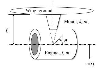
Solution: This combines Examples 1.4.1

kinetic energy is

The kinetic energy in the spring (see example 1.4.4) is

Thus the total kinetic energy is

The potential energy is just

Using the Lagrange formulation of Equation (1.64) the equation of motion results from:

Figure P1.77

and 1.4.4. The

T = 1 mx 2 + 1 Jθ2 + T 1⎛ = ⎜ m + J ⎞ ⎟ x 2 + T 2 2 spring 2⎝ r 2 ⎠ spring

1 m s spring = 2 x 2 3

T =

1⎛ ⎜ m + ⎝ J 2 0 1 m ⎞ ⎟ x  ⎠ U = kx2 2

d ⎛ ∂ ⎛ 1⎛ J m s ⎞ + + ⎞⎞ ∂ ⎛ 1 ⎞ ⎜ ⎜ ⎜ ⎟ x 2 ⎟⎟ + kx2 = 0 dt ⎜ ⎝∂x  ⎝ 2⎝ 2 3 ⎠⎟ ⎠ ∂x 2 ⎛ J s ⎞ ⇒ ⎜ m + 2 + ⎝ 0 ⎟ x  + kx = 0 ⎠ k

1.78 Consider the inverted simple pendulum connected to a spring of Figure P1.68. Use Lagrange’s formulation to derive the equation of motion.

Solution: The energies are (see the solution to 1.68):

Choosing θ as the generalized coordinate, the spring compresses a distance x = l sin

and the mass moves a distance h = l

θ from the reference position. So the Lagrangian becomes:

The terms in Lagrange’s equation

Thus from the Lagrangian the equation of motion is

Where the last expression is the linearized version for small θ.

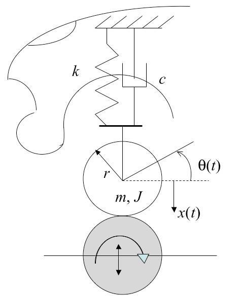
1.79 Lagrange’s formulation can also be used for non-conservative systems by adding the applied non-conservative term to the right side of equation (1.63) to get

Here Ri is the Rayleigh dissipation function defined in the case of a viscous damper attached to ground by

Use this extended Lagrange formulation to derive the equation of motion of the damped automobile suspension driven by a dynamometer illustrated in Figure P1.79. Assume here that the dynamometer drives the system such that x =rθ

T =

2θ 2 , U =

kx2

2 2

1 ml

+ mgh

L = T U = 1 ml2θ 2 1 kl2 sin2θ mgl cosθ 2 2

cos

are ∂L 2  ∂L 2 ∂θ  = ml θ, = kl ∂θ sinθ cosθ + mgl sinθ

d ⎛∂L ⎞ ∂L 2 2 dt ∂θ⎠ ⎟ ∂θ = ml θ + kl sinθcosθ mgl sinθ = 0 ⇒θ + ⎛ lk − mg⎞ ⎝ ml ⎠θ = 0

d ⎛∂T ⎞ ∂T ∂U ∂Ri ⎜ ⎟ + + = 0 dt ⎝∂qi ⎠ ∂qi ∂qi ∂qi

= 1 cq 2 i 2

Solution: The kinetic energy is

The Rayleigh dissipation function is

Lagrange formulation with damping becomes

1.80 Consider the disk of Figure P1.80 connected to two springs. Use the energy method to calculate the system's natural frequency of oscillation for small angles

P1.79

T = 1 mx 2 + 1 Jθ 2 = 1 (m + J )x 2 2 The potential energy is: 2 U = 1 2 2 r 2 kx2

R = 1 cx 2 2

d ⎛∂T ⎞ ∂T ∂U ∂Ri ⎜ ⎟ + + = 0 dt ⎝∂q  i ⎠ ∂qi d ⎛ ∂qi ∂ ⎛ 1 ∂q  i J ⎞⎞ ∂ ⎛ 1 ⎞ ∂ ⎛ 1 ⎞ ⇒ dt ⎜∂x (m + 2 )x 2 r 2 ⎟ + ∂x J kx2 2 + ∂x  cx 2 = 0 2 ⇒ (m + )x  + cx  + kx = 0 r 2

The

θ(t). (t) k s k a r x(t) Figure P1.80 m mass Solution: Known: x = rθ, x ˙ = rθ ˙ and Kinetic energy: J = 1 mr 2 o 2 1 1⎛ mr 2 ⎞ 1 2 2 Trot = 2 J o θ = 2 θ = mr θ 2 4

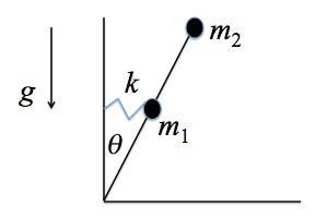
1.81 A pendulum of negligible mass is connected to a spring of stiffness k at halfway along its length, l, as illustrated in Figure P1.81. The pendulum has two masses fixed to it, one at the connection point with the spring and one at the top. Derive the equation of motion using the Lagrange formulation, linearize the equation and compute the systems natural frequency. Assume that the angle remains small enough so that the spring only stretches significantly in the horizontal direction.

Solution: Using the Lagrange formulation the relevant energies are:

From the trigonometry of the drawing:

Figure P1.81

2 T = 1 m ⎛ l ⎞ θ 2 + 1 m l2θ 2 2 1 ⎝ 2⎠ 2 2 U = 1 kx2 + m gh + m gh 2 1 1 2 2

© 2014 Pearson Education, Inc., Upper Saddle River, NJ. All rights reserved. This publication is protected by Copyright and written permission should be obtained from the publisher prior to any prohibited reproduction, storage in a retrieval system, or transmission in any form or by any means, electronic, mechanical, photocopying, recording, or likewise. For information regarding permission(s), write to: Rights and Permissions Department, Pearson Education, Inc., Upper Saddle River, NJ 07458. 2 x = l sinθ, h l = cosθ, h = l cosθ 2 1 2 2 So the potential energy writing in terms of θ is: 2 U = 1 k⎛ l sinθ⎞ + m g l cosθ + m gl cosθ 2 ⎝ 2 ⎠ 1 2 2 Setting L = T-U and taking the derivatives required for the Lagrangian yields: d ⎛∂L ⎞ d ⎛ 1 ⎛ l ⎞ 2 1 2 2⎞ dt ∂θ  ⎠ ⎟ = dt m1 θ 2 ⎝ 2⎠ + m2l θ 2 2 2 d ⎛ 1 2  2 ⎞ m1l + 4m2l  = dt ⎝ 4 m1l θ + m2l θ⎠ = 4 θ ∂L = kl sinθ cosθ l m gsinθ m gl sinθ ∂θ 2 2 1 2 Thus the equation of motion becomes 2 2 m1l + 4m2l θ + kl sinθ cosθ l m gsinθ m gl sinθ = 0 4 2 2 1 2 Linearizing for small θ this becomes 2 2 m1l + 4m2l θ  + (kl l m g m gl)θ = 0 4 So the natural frequency is 2 2 1 2 ω n = 2k 2m1g 4m2g m l + 4m l 1 2

Solutions manual for engineering vibration 4th by inman 0132871696

Engineering Vibration 4th

Articles inside

Engineering Vibration 4th