Artificial Intelligence Hardware Design
Challenges and Solutions
Albert Chun Chen Liu and Oscar Ming Kin Law
Kneron Inc., San Diego, CA, USA
Copyright © 2021 by The Institute of Electrical and Electronics Engineers, Inc. All rights reserved.
Published by John Wiley & Sons, Inc., Hoboken, New Jersey. Published simultaneously in Canada.
No part of this publication may be reproduced, stored in a retrieval system, or transmitted in any form or by any means, electronic, mechanical, photocopying, recording, scanning, or otherwise, except as permitted under Section 107 or 108 of the 1976 United States Copyright Act, without either the prior written permission of the Publisher, or authorization through payment of the appropriate per-copy fee to the Copyright Clearance Center, Inc., 222 Rosewood Drive, Danvers, MA 01923, (978) 750-8400, fax (978) 750-4470, or on the web at www.copyright. com. Requests to the Publisher for permission should be addressed to the Permissions Department, John Wiley & Sons, Inc., 111 River Street, Hoboken, NJ 07030, (201) 748-6011, fax (201) 748-6008, or online at http://www.wiley.com/go/permission.
Limit of Liability/Disclaimer of Warranty: While the publisher and author have used their best efforts in preparing this book, they make no representations or warranties with respect to the accuracy or completeness of the contents of this book and specifically disclaim any implied warranties of merchantability or fitness for a particular purpose. No warranty may be created or extended by sales representatives or written sales materials. The advice and strategies contained herein may not be suitable for your situation. You should consult with a professional where appropriate. Neither the publisher nor author shall be liable for any loss of profit or any other commercial damages, including but not limited to special, incidental, consequential, or other damages.
For general information on our other products and services or for technical support, please contact our Customer Care Department within the United States at (800) 762-2974, outside the United States at (317) 572-3993 or fax (317) 572-4002.
Wiley also publishes its books in a variety of electronic formats. Some content that appears in print may not be available in electronic formats. For more information about Wiley products, visit our web site at www.wiley.com.
Library of Congress Cataloging-in-Publication data applied for:
ISBN: 9781119810452
Cover design by Wiley
Cover image: © Rasi Bhadramani/iStock/Getty Images
Set in 9.5/12.5pt STIXTwoText by Straive, Pondicherry, India
Contents
Author Biographies xi
Preface xiii
Acknowledgments xv
Table of Figures xvii
1 Introduction 1
1.1 Development History 2
1.2 Neural Network Models 4
1.3 Neural Network Classification 4
1.3.1 Supervised Learning 4
1.3.2 Semi-supervised Learning 5
1.3.3 Unsupervised Learning 6
1.4 Neural Network Framework 6
1.5 Neural Network Comparison 10
Exercise 11
References 12
2 Deep Learning 13
2.1 Neural Network Layer 13
2.1.1 Convolutional Layer 13
2.1.2 Activation Layer 17
2.1.3 Pooling Layer 18
2.1.4 Normalization Layer 19
2.1.5 Dropout Layer 20
2.1.6 Fully Connected Layer 20
2.2 Deep Learning Challenges 22 Exercise 22
References 24
3 Parallel Architecture 25
3.1 Intel Central Processing Unit (CPU) 25
3.1.1 Skylake Mesh Architecture 27
3.1.2 Intel Ultra Path Interconnect (UPI) 28
3.1.3 Sub Non-unified Memory Access Clustering (SNC) 29
3.1.4 Cache Hierarchy Changes 31
3.1.5 Single/Multiple Socket Parallel Processing 32
3.1.6 Advanced Vector Software Extension 33
3.1.7 Math Kernel Library for Deep Neural Network (MKL-DNN) 34
3.2 NVIDIA Graphics Processing Unit (GPU) 39
3.2.1 Tensor Core Architecture 41
3.2.2 Winograd Transform 44
3.2.3 Simultaneous Multithreading (SMT) 45
3.2.4 High Bandwidth Memory (HBM2) 46
3.2.5 NVLink2 Configuration 47
3.3 NVIDIA Deep Learning Accelerator (NVDLA) 49
3.3.1 Convolution Operation 50
3.3.2 Single Data Point Operation 50
3.3.3 Planar Data Operation 50
3.3.4 Multiplane Operation 50
3.3.5 Data Memory and Reshape Operations 51
3.3.6 System Configuration 51
3.3.7 External Interface 52
3.3.8 Software Design 52
3.4 Google Tensor Processing Unit (TPU) 53
3.4.1 System Architecture 53
3.4.2 Multiply–Accumulate (MAC) Systolic Array 55
3.4.3 New Brain Floating-Point Format 55
3.4.4 Performance Comparison 57
3.4.5 Cloud TPU Configuration 58
3.4.6 Cloud Software Architecture 60
3.5 Microsoft Catapult Fabric Accelerator 61
3.5.1 System Configuration 64
3.5.2 Catapult Fabric Architecture 65
3.5.3 Matrix-Vector Multiplier 65
3.5.4 Hierarchical Decode and Dispatch (HDD) 67
3.5.5 Sparse Matrix-Vector Multiplication 68 Exercise 70 References 71
4 Streaming Graph Theory 73
4.1 Blaize Graph Streaming Processor 73
4.1.1 Stream Graph Model 73
4.1.2 Depth First Scheduling Approach 75
4.1.3 Graph Streaming Processor Architecture 76
4.2 Graphcore Intelligence Processing Unit 79
4.2.1 Intelligence Processor Unit Architecture 79
4.2.2 Accumulating Matrix Product (AMP) Unit 79
4.2.3 Memory Architecture 79
4.2.4 Interconnect Architecture 79
4.2.5 Bulk Synchronous Parallel Model 81
Exercise 83 References 84
5 Convolution Optimization 85
5.1 Deep Convolutional Neural Network Accelerator 85
5.1.1 System Architecture 86
5.1.2 Filter Decomposition 87
5.1.3 Streaming Architecture 90
5.1.3.1 Filter Weights Reuse 90
5.1.3.2 Input Channel Reuse 92
5.1.4 Pooling 92
5.1.4.1 Average Pooling 92
5.1.4.2 Max Pooling 93
5.1.5 Convolution Unit (CU) Engine 94
5.1.6 Accumulation (ACCU) Buffer 94
5.1.7 Model Compression 95
5.1.8 System Performance 95
5.2 Eyeriss Accelerator 97
5.2.1 Eyeriss System Architecture 97
5.2.2 2D Convolution to 1D Multiplication 98
5.2.3 Stationary Dataflow 99
5.2.3.1 Output Stationary 99
5.2.3.2 Weight Stationary 101
5.2.3.3 Input Stationary 101
5.2.4 Row Stationary (RS) Dataflow 104
5.2.4.1 Filter Reuse 104
5.2.4.2 Input Feature Maps Reuse 106
5.2.4.3 Partial Sums Reuse 106
5.2.5 Run-Length Compression (RLC) 106
5.2.6 Global Buffer 108
5.2.7 Processing Element Architecture 108
5.2.8 Network-on- Chip (NoC) 108
5.2.9 Eyeriss v2 System Architecture 112
5.2.10 Hierarchical Mesh Network 116
5.2.10.1 Input Activation HM-NoC 118
5.2.10.2 Filter Weight HM-NoC 118
5.2.10.3 Partial Sum HM-NoC 119
5.2.11 Compressed Sparse Column Format 120
5.2.12 Row Stationary Plus (RS+) Dataflow 122
5.2.13 System Performance 123 Exercise 125
References 125
6 In-Memory Computation 127
6.1 Neurocube Architecture 127
6.1.1 Hybrid Memory Cube (HMC) 127
6.1.2 Memory Centric Neural Computing (MCNC) 130
6.1.3 Programmable Neurosequence Generator (PNG) 131
6.1.4 System Performance 132
6.2 Tetris Accelerator 133
6.2.1 Memory Hierarchy 133
6.2.2 In-Memory Accumulation 133
6.2.3 Data Scheduling 135
6.2.4 Neural Network Vaults Partition 136
6.2.5 System Performance 137
6.3 NeuroStream Accelerator 138
6.3.1 System Architecture 138
6.3.2 NeuroStream Coprocessor 140
6.3.3 4D Tiling Mechanism 140
6.3.4 System Performance 141 Exercise 143
References 143
7 Near-Memory Architecture 145
7.1 DaDianNao Supercomputer 145
7.1.1 Memory Configuration 145
7.1.2 Neural Functional Unit (NFU) 146
7.1.3 System Performance 149
7.2 Cnvlutin Accelerator 150
7.2.1 Basic Operation 151
7.2.2 System Architecture 151
7.2.3 Processing Order 154
7.2.4 Zero-Free Neuron Array Format (ZFNAf) 155
7.2.5 The Dispatcher 155
7.2.6 Network Pruning 157
7.2.7 System Performance 157
7.2.8 Raw or Encoded Format (RoE) 158
7.2.9 Vector Ineffectual Activation Identifier Format (VIAI) 159
7.2.10 Ineffectual Activation Skipping 159
7.2.11 Ineffectual Weight Skipping 161
Exercise 161
References 161
8 Network Sparsity 163
8.1 Energy Efficient Inference Engine (EIE) 163
8.1.1 Leading Nonzero Detection (LNZD) Network 163
8.1.2 Central Control Unit (CCU) 164
8.1.3 Processing Element (PE) 164
8.1.4 Deep Compression 166
8.1.5 Sparse Matrix Computation 167
8.1.6 System Performance 169
8.2 Cambricon-X Accelerator 169
8.2.1 Computation Unit 171
8.2.2 Buffer Controller 171
8.2.3 System Performance 174
8.3 SCNN Accelerator 175
8.3.1 SCNN PT-IS- CP-Dense Dataflow 175
8.3.2 SCNN PT-IS- CP-Sparse Dataflow 177
8.3.3 SCNN Tiled Architecture 178
8.3.4 Processing Element Architecture 179
8.3.5 Data Compression 180
8.3.6 System Performance 180
8.4 SeerNet Accelerator 183
8.4.1 Low-Bit Quantization 183
8.4.2 Efficient Quantization 184
8.4.3 Quantized Convolution 185
8.4.4 Inference Acceleration 186
8.4.5 Sparsity-Mask Encoding 186
8.4.6 System Performance 188
Exercise 188
References 188
9 3D Neural Processing 191
9.1 3D Integrated Circuit Architecture 191
9.2 Power Distribution Network 193
9.3 3D Network Bridge 195
9.3.1 3D Network-on- Chip 195
9.3.2 Multiple- Channel High-Speed Link 195
9.4 Power-Saving Techniques 198
9.4.1 Power Gating 198
9.4.2 Clock Gating 199
Exercise 200
References 201
Appendix A: Neural Network Topology 203
Index 205
Author Biographies
Albert Chun Chen Liu is Kneron’s founder and CEO. He is Adjunct Associate Professor at National Tsing Hua University, National Chiao Tung University, and National Cheng Kung University. After graduating from the Taiwan National Cheng Kung University, he got scholarships from Raytheon and the University of California to join the UC Berkeley/UCLA/UCSD research programs and then earned his Ph.D. in Electrical Engineering from the University of California Los Angeles (UCLA). Before establishing Kneron in San Diego in 2015, he worked in R&D and management positions in Qualcomm, Samsung Electronics R&D Center, MStar, and Wireless Information.
Albert has been invited to give lectures on computer vision technology and artificial intelligence at the University of California and be a technical reviewer for many internationally renowned academic journals. Also, Albert owned more than 30 international patents in artificial intelligence, computer vision, and image processing. He has published more than 70 papers. He is a recipient of the IBM Problem Solving Award based on the use of the EIP tool suite in 2007 and IEEE TCAS Darlington award in 2021.
Oscar Ming Kin Law developed his interest in smart robot development in 2014. He has successfully integrated deep learning with the self-driving car, smart drone, and robotic arm. He is currently working on humanoid development. He received a Ph.D. in Electrical and Computer Engineering from the University of Toronto, Canada.
Oscar currently works at Kneron for in-memory computing and smart robot development. He has worked at ATI Technologies, AMD, TSMC, and Qualcomm and led various groups for chip verification, standard cell design, signal integrity, power analysis, and Design for Manufacturability (DFM). He has conducted different seminars at the University of California, San Diego, University of Toronto, Qualcomm, and TSMC. He has also published over 60 patents in various areas.
Preface
With the breakthrough of the Convolutional Neural Network (CNN) for image classification in 2012, Deep Learning (DL) has successfully solved many complex problems and widely used in our everyday life, automotive, finance, retail, and healthcare. In 2016, Artificial Intelligence (AI) exceeded human intelligence that Google AlphaGo won the GO world championship through Reinforcement Learning (RL). AI revolution gradually changes our world, like a personal computer (1977), Internet (1994), and smartphone (2007). However, most of the efforts focus on software development rather than hardware challenges:
● Big input data
● Deep neural network
● Massive parallel processing
● Reconfigurable network
● Memory bottleneck
● Intensive computation
● Network pruning
● Data sparsity
This book shows how to resolve the hardware problems through various design ranging from CPU, GPU, TPU to NPU. Novel hardware can be evolved from those designs for further performance and power improvement:
● Parallel architecture
● Streaming Graph Theory
● Convolution optimization
● In-memory computation
● Near-memory architecture
● Network sparsity
● 3D neural processing
Organization of the Book
Chapter 1 introduces neural network and discusses neural network development history.
Chapter 2 reviews Convolutional Neural Network (CNN) model and describes each layer functions and examples.
Chapter 3 lists out several parallel architectures, Intel CPU, Nvidia GPU, Google TPU, and Microsoft NPU. It emphasizes hardware/software integration for performance improvement. Nvidia Deep Learning Accelerator (NVDLA) opensource project is chosen for FPGA hardware implementation.
Chapter 4 introduces a streaming graph for massive parallel computation through Blaize GSP and Graphcore IPU. They apply the Depth First Search (DFS) for task allocation and Bulk Synchronous Parallel Model (BSP) for parallel operations.
Chapter 5 shows how to optimize convolution with the University of California, Los Angeles (UCLA) Deep Convolutional Neural Network (DCNN) accelerator filter decomposition and Massachusetts Institute of Technology (MIT) Eyeriss accelerator Row Stationary dataflow.
Chapter 6 illustrates in-memory computation through Georgia Institute of Technologies Neurocube and Stanford Tetris accelerator using Hybrid Memory Cube (HMC) as well as University of Bologna Neurostream accelerator using Smart Memory Cubes (SMC).
Chapter 7 highlights near-memory architecture through the Institute of Computing Technology (ICT), Chinese Academy of Science, DaDianNao supercomputer and University of Toronto Cnvlutin accelerator. It also shows Cnvlutin how to avoid ineffectual zero operations.
Chapter 8 chooses Stanford Energy Efficient Inference Engine, Institute of Computing Technology (ICT), Chinese Academy of Science Cambricon-X, Massachusetts Institute of Technology (MIT) SCNN processor and Microsoft SeerNet accelerator to handle network sparsity.
Chapter 9 introduces an innovative 3D neural processing with a network bridge to overcome power and thermal challenges. It also solves the memory bottleneck and handles the large neural network processing.
In English edition, several chapters are rewritten with more detailed descriptions. New deep learning hardware architectures are also included. Exercises challenge the reader to solve the problems beyond the scope of this book. The instructional slides are available upon request.
We shall continue to explore different deep learning hardware architectures (i.e. Reinforcement Learning) and work on a in-memory computing architecture with new high-speed arithmetic approach. Compared with the Google Brain floatingpoint (BFP16) format, the new approach offers a wider dynamic range, higher performance, and less power dissipation. It will be included in a future revision.
Albert Chun Chen Liu Oscar Ming Kin Law
Acknowledgments
First, we would like to thank all who have supported the publication of the book. We are thankful to Iain Law and Enoch Law for the manuscript preparation and project development. We would like to thank Lincoln Lee and Amelia Leung for reviewing the content. We also thank Claire Chang, Charlene Jin, and Alex Liao for managing the book production and publication. In addition, we are grateful to the readers of the Chinese edition for their valuable feedback on improving the content of this book. Finally, we would like to thank our families for their support throughout the publication of this book.
Albert Chun Chen Liu Oscar Ming Kin Law
Table of Figures
1.1 High-tech revolution 2
1.2 Neural network development timeline 2
1.3 ImageNet challenge 3
1.4 Neural network model 5
1.5 Regression 6
1.6 Clustering 7
1.7 Neural network top 1 accuracy vs. computational complexity 9
1.8 Neural network top 1 accuracy density vs. model efficiency [14] 10
1.9 Neural network memory utilization and computational complexity [14] 11
2.1 Deep neural network AlexNet architecture [1] 14
2.2 Deep neural network AlexNet model parameters 15
2.3 Deep neural network AlexNet feature map evolution [3] 15
2.4 Convolution function 16
2.5 Nonlinear activation functions 18
2.6 Pooling functions 19
2.7 Dropout layer 20
2.8 Deep learning hardware issues [1] 21
3.1 Intel Xeon processor ES 2600 family Grantley platform ring architecture [3] 27
3.2 Intel Xeon processor scalable family Purley platform mesh architecture [3] 28
3.3 Two-socket configuration 28
3.4 Four-socket ring configuration 29
3.5 Four-socket crossbar configuration 29
3.6 Eight-socket configuration 30
3.7 Sub-NUMA cluster domains [3] 31
3.8 Cache hierarchy comparison 31
3.9 Intel multiple sockets parallel processing 32
Table of Figures
3.10
3.11
3.12
Intel multiple socket training performance comparison [4] 32
Intel AVX-512 16 bits FMA operations (VPMADDWD + VPADDD) 33
Intel AVX-512 with VNNI 16 bits FMA operation (VPDPWSSD) 34
3.13 Intel low-precision convolution 35
3.14 Intel Xenon processor training throughput comparison [2] 38
3.15 Intel Xenon processor inference throughput comparison [2] 39
3.16 NVIDIA turing GPU architecture 40
3.17 NVIDIA GPU shared memory 41
3.18 Tensor core 4 × 4 × 4 matrix operation [9] 42
3.19 Turing tensor core performance [7] 42
3.20 Matrix D thread group indices 43
3.21 Matrix D 4 × 8 elements computation 43
3.22 Different size matrix multiplication 44
3.23 Simultaneous multithreading (SMT) 45
3.24 Multithreading schedule 46
3.25 GPU with HBM2 architecture 46
3.26 Eight GPUs NVLink2 configuration 47
3.27 Four GPUs NVLink2 configuration 48
3.28 Two GPUs NVLink2 configuration 48
3.29 Single GPU NVLink2 configuration 48
3.30 NVDLA core architecture 49
3.31 NVDLA small system model 51
3.32 NVDLA large system model 51
3.33 NVDLA software dataflow 52
3.34 Tensor processing unit architecture 54
3.35 Tensor processing unit floorplan 55
3.36 Multiply–Accumulate (MAC) systolic array 56
3.37 Systolic array matrix multiplication 56
3.38 Cost of different numerical format operation 57
3.39 TPU brain floating-point format 57
3.40 CPU, GPU, and TPU performance comparison [15] 58
3.41 Tensor Processing Unit (TPU) v1 59
3.42 Tensor Processing Unit (TPU) v2 59
3.43 Tensor Processing Unit (TPU) v3 59
3.44 Google TensorFlow subgraph optimization 61
3.45 Microsoft Brainwave configurable cloud architecture 62
3.46 Tour network topology 63
3.47 Microsoft Brainwave design flow 63
3.48 The Catapult fabric shell architecture 64
3.49 The Catapult fabric microarchitecture 65
3.50 Microsoft low-precision quantization [27] 66
Table of Figures
3.51 Matrix-vector multiplier overview 66
3.52 Tile engine architecture 67
3.53 Hierarchical decode and dispatch scheme 68
3.54 Sparse matrix-vector multiplier architecture 69
3.55 (a) Sparse Matrix; (b) CSR Format; and (c) CISR Format 70
4.1 Data streaming TCS model 74
4.2 Blaize depth-first scheduling approach 75
4.3 Blaize graph streaming processor architecture 76
4.4 Blaize GSP thread scheduling 76
4.5 Blaize GSP instruction scheduling 77
4.6 Streaming vs. sequential processing comparison 77
4.7 Blaize GSP convolution operation 78
4.8 Intelligence processing unit architecture [8] 80
4.9 Intelligence processing unit mixed-precision multiplication 81
4.10 Intelligence processing unit single-precision multiplication 81
4.11 Intelligence processing unit interconnect architecture [9] 81
4.12 Intelligence processing unit bulk synchronous parallel model 82
4.13 Intelligence processing unit bulk synchronous parallel execution trace [9] 82
4.14 Intelligence processing unit bulk synchronous parallel inter-chip execution [9] 83
5.1 Deep convolutional neural network hardware architecture 86
5.2 Convolution computation 87
5.3 Filter decomposition with zero padding 88
5.4 Filter decomposition approach 89
5.5 Data streaming architecture with the data flow 91
5.6 DCNN accelerator COL buffer architecture 91
5.7 Data streaming architecture with 1×1 convolution mode 92
5.8 Max pooling architecture 93
5.9 Convolution engine architecture 94
5.10 Accumulation (ACCU) buffer architecture 95
5.11 Neural network model compression 96
5.12 Eyeriss system architecture 97
5.13 2D convolution to 1D multiplication mapping 98
5.14 2D convolution to 1D multiplication – step #1 99
5.15 2D convolution to 1D multiplication – step #2 100
5.16 2D convolution to 1D multiplication – step #3 100
5.17 2D convolution to 1D multiplication – step #4 101
5.18 Output stationary 102
5.19 Output stationary index looping 102
5.20 Weight stationary 103
Table of Figures xx
5.21 Weight stationary index looping 103
5.22 Input stationary 104
5.23 Input stationary index looping 104
5.24 Eyeriss Row Stationary (RS) dataflow 105
5.25 Filter reuse 106
5.26 Feature map reuse 107
5.27 Partial sum reuse 107
5.28 Eyeriss run-length compression 108
5.29 Eyeriss processing element architecture 109
5.30 Eyeriss global input network 109
5.31 Eyeriss processing element mapping (AlexNet CONV1) 110
5.32 Eyeriss processing element mapping (AlexNet CONV2) 111
5.33 Eyeriss processing element mapping (AlexNet CONV3) 111
5.34 Eyeriss processing element mapping (AlexNet CONV4/CONV5) 112
5.35 Eyeriss processing element operation (AlexNet CONV1) 112
5.36 Eyeriss processing element operation (AlexNet CONV2) 113
5.37 Eyeriss processing element (AlexNet CONV3) 113
5.38 Eyeriss processing element operation (AlexNet CONV4/CONV5) 114
5.39 Eyeriss architecture comparison 114
5.40 Eyeriss v2 system architecture 115
5.41 Network-on- Chip configurations 116
5.42 Mesh network configuration 117
5.43 Eyeriss v2 hierarchical mesh network examples 117
5.44 Eyeriss v2 input activation hierarchical mesh network 118
5.45 Weights hierarchical mesh network 119
5.46 Eyeriss v2 partial sum hierarchical mesh network 120
5.47 Eyeriss v1 neural network model performance [6] 120
5.48 Eyeriss v2 neural network model performance [6] 121
5.49 Compressed sparse column format 121
5.50 Eyeriss v2 PE architecture 122
5.51 Eyeriss v2 row stationary plus dataflow 123
5.52 Eyeriss architecture AlexNet throughput speedup [6] 124
5.53 Eyeriss architecture AlexNet energy efficiency [6] 124
5.54 Eyeriss architecture MobileNet throughput speedup [6] 124
5.55 Eyeriss architecture MobileNet energy efficiency [6] 125
6.1 Neurocube architecture 128
6.2 Neurocube organization 128
6.3 Neurocube 2D mesh network 129
6.4 Memory-centric neural computing flow 130
6.5 Programmable neurosequence generator architecture 131
6.6 Neurocube programmable neurosequence generator 131
Table of Figures xxi
6.7 Tetris system architecture 134
6.8 Tetris neural network engine 134
6.9 In-memory accumulation 135
6.10 Global buffer bypass 136
6.11 NN partitioning scheme comparison 137
6.12 Tetris performance and power comparison [7] 138
6.13 NeuroStream and NeuroCluster architecture 139
6.14 NeuroStream coprocessor architecture 140
6.15 NeuroStream 4D tiling 142
6.16 NeuroStream roofline plot [8] 142
7.1 DaDianNao system architecture 146
7.2 DaDianNao neural functional unit architecture 147
7.3 DaDianNao pipeline configuration 148
7.4 DaDianNao multi-node mapping 148
7.5 DaDianNao timing performance (Training) [1] 149
7.6 DaDianNao timing performance (Inference) [1] 149
7.7 DaDianNao power reduction (Training) [1] 150
7.8 DaDianNao power reduction (Inference) [1] 150
7.9 DaDianNao basic operation 152
7.10 Cnvlutin basic operation 153
7.11 DaDianNao architecture 153
7.12 Cnvlutin architecture 154
7.13 DaDianNao processing order 155
7.14 Cnvlutin processing order 156
7.15 Cnvlutin zero free neuron array format 157
7.16 Cnvlutin dispatch 157
7.17 Cnvlutin timing comparison [4] 158
7.18 Cnvlutin power comparison [4] 158
7.19 Cnvlutin2 ineffectual activation skipping 159
7.20 Cnvlutin2 ineffectual weight skipping 160
8.1 EIE leading nonzero detection network 164
8.2 EIE processing element architecture 165
8.3 Deep compression weight sharing and quantization 166
8.4 Matrix W, vector a and b are interleaved over four processing elements 168
8.5 Matrix W layout in compressed sparse column format 169
8.6 EIE timing performance comparison [1] 170
8.7 EIE energy efficient comparison [1] 170
8.8 Cambricon-X architecture 171
8.9 Cambricon-X processing element architecture 172
8.10 Cambricon-X sparse compression 172
8.11 Cambricon-X buffer controller architecture 173
Table of Figures
8.12
8.13
Cambricon-X index module architecture 173
Cambricon-X direct indexing architecture 174
8.14 Cambricon-X step indexing architecture 174
8.15
Cambricon-X timing performance comparison [4] 175
8.16 Cambricon-X energy efficiency comparison [4] 175
8.17 SCNN convolution 176
8.18 SCNN convolution nested loop 176
8.19 PT-IS- CP-dense dataflow 178
8.20 SCNN architecture 179
8.21 SCNN dataflow 179
8.22 SCNN weight compression 180
8.23 SCNN timing performance comparison [5] 181
8.24 SCNN energy efficiency comparison [5] 182
8.25 SeerNet architecture 183
8.26 SeerNet Q-ReLU and Q-max-pooling 184
8.27 SeerNet quantization 185
8.28 SeerNet sparsity-mask encoding 187
9.1 2.5D interposer architecture 192
9.2 3D stacked architecture 192
9.3 3D-IC PDN configuration (pyramid shape) 192
9.4 PDN – Conventional PDN Manthan geometry 194
9.5 Novel PDN X topology 194
9.6 3D network bridge 196
9.7 Neural network layer multiple nodes connection 197
9.8 3D network switch 197
9.9 3D network bridge segmentation 197
9.10 Multiple-channel bidirectional high-speed link 198
9.11 Power switch configuration 199
9.12 3D neural processing power gating approach 199
9.13 3D neural processing clock gating approach 200
1
Introduction
With the advancement of Deep Learning (DL) for image classification in 2012 [1], Convolutional Neural Network (CNN) extracted the image features and successfully classified the objects. It reduced the error rate by 10% compared with the traditional computer vision algorithmic approaches. Finally, ResNet showed the error rate better than human 5% accuracy in 2015. Different Deep Neural Network (DNN) models are developed for various applications ranging from automotive, finance, retail to healthcare. They have successfully solved complex problems and widely used in our everyday life. For example, Tesla autopilot guides the driver for lane changes, navigating interchanges, and highway exit. It will support traffic sign recognition and city automatic driving in near future.
In 2016, Google AlphaGo won the GO world championship through Reinforcement Learning (RL) [2]. It evaluated the environment, decided the action, and, finally, won the game. RL has large impacts on robot development because the robot adapts to the changes in the environment through learning rather than programming. It expands the robot role in industrial automation. The Artificial Intelligent (AI) revolution has gradually changed our world, like a personal computer (1977)1, the Internet (1994)2 and smartphone (2007).3 It significantly improves the human living (Figure 1.1).
1 Apple IIe (1997) and IBM PC (1981) provided the affordable hardware for software development, new software highly improved the working efficiency in our everyday life and changed our world.
2 The information superhighway (1994) connects the whole world through the Internet that improves personal-to-personal communication. Google search engine makes the information available at your fingertips.
3 Apple iPhone (2007) changed the phone to the multimedia platform. It not only allows people to listen to the music and watch the video, but also integrates many utilities (i.e. e-mail, calendar, wallet, and note) into the phone.
Artificial Intelligence Hardware Design: Challenges and Solutions, First Edition. Albert Chun Chen Liu and Oscar Ming Kin Law.
© 2021 The Institute of Electrical and Electronics Engineers, Inc. Published 2021 by John Wiley & Sons, Inc.
1977
Inter net
Smar tphone Deep lear ning
Figure 1.1 High-tech revolution.
1.1 Development History
Neural Network [3] had been developed for a long time. In 1943, the first computer Electronic Numerical Integrator and Calculator (ENIAC) was constructed at the University of Pennsylvania. At the same time, a neurophysiologist, Warren McCulloch, and a mathematician, Walter Pitts, described how neurons might work [4] and modeled a simple neural network using an electrical circuit. In 1949, Donald Hebb wrote the book, The Organization of Behavior, which pointed out how the neural network is strengthened through practice (Figure 1.2).
In the 1950s, Nathanial Rochester simulated the first neural network in IBM Research Laboratory. In 1956, the Dartmouth Summer Research Project on Artificial Intelligence linked up artificial intelligence (AI) with neural network for joint project development. In the following year, John von Neumann suggested to implement simple neuron functions using telegraph relays or vacuum tubes. Also,
1950s
Simulate First Neural Net work Rockester
1943 Neural Net work
McCullock & Pitt
1959 ADALINE + MADLINE
Widrow & Hoff
1957 Neuron Implementation von Neuman
1987
IEEE Neural Net work Conference
1982
Hopfield Net work Hopfield
2015 ResNet Error < 5%
He
1997 Convolutional Neural Net work LeCun
1956 Ar tifical Intelligence + Neural Net work
1949 The Organization of Behavior Book Hebb
1969 Perceptron Book
Minsky & Paper t
1958 Perceptron Rosenblatt
1997
Recurrent Neural Net work (LSTM) Schmidhuber & Hochreiter
1985 Neural Net work for Computing American Institue of Physics
Figure 1.2 Neural network development timeline.
2012 AlexNet Krizhevsky
a neurobiologist from Cornell University, Frank Rosenblatt, worked on Perceptron [5], which is a single-layer perceptron to classify the results from two classes. The perception computes the weighted sum of the inputs and subtracts a threshold, and then outputs one of two possible results. Perception is the oldest neural network model still used today. However, Marvin Minsky and Seymour Papert published the book, Perceptron [6], to show the limitation of perception in 1969.
In 1959, Bernard Widrow and Marcian Hoff from Stanford University developed Multiple ADaptive LINear Elements called ADALINE and MADALINE, which were adaptive filter to eliminate the echoes in the phone line. Due to unmatured electronics and fear the machine impacts toward humans, neural network development was halted for a decade.
Until 1982, John Hopfield presented a new neural network model, the Hopfield neural network [7], with the mathematical analysis in the National Academy of Sciences. At the same time, the United States started to fund neural network research to compete with Japan after Japan announced fifth-generation AI research in the US-Japan Cooperative/Competitive Neural Networks’ joint conference. In 1985, the American Institute of Physics started the annual meeting, Neural Network for Computing. By 1987, the first IEEE neural network international conference took place with 1800 attendees. In 1997, Schmidhuber and Hochreiter proposed a recurrent neural network model with Long-Short Term Memory (LSTM) useful for future time series speech processing. In 1997, Yann LeCun published Gradient-Based Learning Applied to Document Recognition [8]. It introduced the CNN that laid the foundation for modern DNN development (Figure 1.3).
During ImageNet Large Scale Visual Recognition Challenge (ILSVRC 2012) [9], University of Toronto researchers applied CNN Model, AlexNet [1], successfully recognized the object and achieved a top-5 error rate 10% better than traditional computer vision algorithmic approaches. For ILSVRC, there are over 14 million images with 21 thousand classes and more than 1 million images with bounding box. The competition focused on 1000 classes with a trimmed database for image classification and object detection. For image classification, the class label is assigned to the object in the images and it localizes the object with a bounding box for object detection. With the evolution of DNN models, Clarifia [10], VGG-16 [11], and GoogleNet [12], the error rate was rapidly reduced. In 2015, ResNet [13] showed an error rate of less than 5% of human level accuracy. The rapid growth of deep learning is transforming our world.
1.2 Neural Network Models
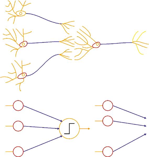
The brain consists of 86 billion neurons and each neuron has a cell body (or soma) to control the function of the neuron. Dendrites are the branch-like structures extending away from the cell body responsible for neuron communication. It receives the message from other neurons and allows the message to travel to the cell body. An axon carries an electric impulse from the cell body to the opposite end of the neuron, an axon terminal that passes the impulse to another neuron. The synapse is the chemical junction between the axon terminal of one neuron and dendrite where the chemical reaction occurs, excited and inhibited. It decides how to transmit the message between the neurons. The structure of a neuron allows the brain to transmit the message to the rest of the body and control all the actions (Figure 1.4).
The neural network model is derived from a human neuron. It consists of the node, weight, and interconnect. The node (cell body) controls the neural network operation and performs the computation. The weight (axon) connects to either a single node or multiple ones for signal transfer. The activation (synapse) decides the signal transfer from one node to others.
1.3 Neural Network Classification
The neural network models are divided into supervised, semi-supervised, and unsupervised learning.
1.3.1
Supervised Learning
Supervised learning sets the desired output and trains with a particular input dataset to minimize the error between the desired and predicted outputs. After the
successful training, the network predicts the outputs based on unknown inputs. The popular supervised models are CNN and Recurrent Neural Network (RNN) including Long Short-Term Memory Network (LSTM).
Regression is typically used for supervised learning; it predicts the value based on the input dataset and finds the relationship between the input and output. Linear regression is the popular regression approach (Figure 1.5).
1.3.2 Semi-supervised Learning
Semi-supervised learning is based on partial labeled output for training where Reinforcement Learning (RL) is the best example. Unlabeled data is mixed with a small amount of labeled data that can improve learning accuracy under a different environment.
Figure 1.4 Neural network model.
Figure 1.5 Regression.
1.3.3 Unsupervised Learning
Unsupervised learning is the network that learns the important features from the dataset which exploits the relationship among the inputs through clustering, dimensionality reduction, and generative techniques. The examples include Auto Encoder (AE), Restricted Boltzmann Machine (RBM), and Deep Belief Network (DBN).
Clustering is a useful technique for unsupervised learning. It divides the dataset into multiple groups where the data points are similar to each other in the same group. The popular clustering algorithm is k-means technique (Figure 1.6).
1.4 Neural Network Framework
The software frameworks are developed to support deep learning applications. The most popular academic framework is Caffe which is migrated into Pytorch. Pytorch is a deep learning research platform that provides maximum flexibility and speed. It replaces NumPy package to fully utilize GPU computational resource. TensorFlow is a dataflow symbolic library used for industrial