Download full Mechanics of materials 9th edition ebook all chapters

Page 1


Mechanics of Materials 9th Edition

Visit to download the full and correct content document: https://ebookmass.com/product/mechanics-of-materials-9th-edition/

More products digital (pdf, epub, mobi) instant download maybe you interests ...

Mechanics of Materials 9th Edition Barry J. Goodno

https://ebookmass.com/product/mechanics-of-materials-9th-editionbarry-j-goodno/

Mechanics Of Materials 7th Edition Beer

https://ebookmass.com/product/mechanics-of-materials-7th-editionbeer/

Mechanics of materials Ninth Edition, Si. Edition Gere

https://ebookmass.com/product/mechanics-of-materials-ninthedition-si-edition-gere/

eTextbook 978-0134319650 Mechanics of Materials (10th Edition)

https://ebookmass.com/product/etextbook-978-0134319650-mechanicsof-materials-10th-edition/

Statics and Mechanics of Materials (5th Edition ) 5th Edition

https://ebookmass.com/product/statics-and-mechanics-ofmaterials-5th-edition-5th-edition/

eTextbook 978-0134382593 Statics and Mechanics of Materials (5th Edition)

https://ebookmass.com/product/etextbook-978-0134382593-staticsand-mechanics-of-materials-5th-edition/

Statics and Mechanics of Materials 2nd Edition

Ferdinand P. Beer

https://ebookmass.com/product/statics-and-mechanics-ofmaterials-2nd-edition-ferdinand-p-beer/

Fluid Mechanics (9th Edition) Frank M. White

https://ebookmass.com/product/fluid-mechanics-9th-edition-frankm-white/

Munson, Young and Okiishi's Fundamentals of Fluid Mechanics 9th Edition Philip M. Gerhart

https://ebookmass.com/product/munson-young-and-okiishisfundamentals-of-fluid-mechanics-9th-edition-philip-m-gerhart/

5.4 Longitudinal Strains in Beams 449

5.5 Normal Stress in Beams (Linearly Elastic Materials) 453

5.6 Design of Beams for Bending Stresses 466

5.7 Nonprismatic Beams 476

5.8 Shear Stresses in Beams of Rectangular Cross Section 480

5.9 Shear Stresses in Beams of Circular Cross Section 488

5.10 Shear Stresses in the Webs of Beams with Flanges 491

*5.11 Built-Up Beams and Shear Flow 498

*5.12 Beams with Axial Loads 502

*5.13 Stress Concentrations in Bending 509

Chapter Summary and Review 514 Problems 518

6. Stresses in Beams (Advanced Topics) 553

6.1 Introduction 554

6.2 Composite Beams 554

6.3 Transformed-Section Method 563

6.4 Doubly Symmetric Beams with Inclined Loads 571

6.5 Bending of Unsymmetric Beams 578

6.6 The Shear-Center Concept 589

6.7 Shear Stresses in Beams of Thin-Walled Open Cross Sections 590

6.8 Shear Stresses in Wide-Flange Beams 593

6.9 Shear Centers of Thin-Walled Open Sections 597

*6.10 Elastoplastic Bending 605

Chapter Summary and Review 614 Problems 616

7. Analysis of Stress and Strain 639

7.1 Introduction 640

7.2 Plane Stress 640

7.3 Principal Stresses and Maximum Shear Stresses 648

7.4 Mohr’s Circle for Plane Stress 656

7.5 Hooke’s Law for Plane Stress 669

7.6 Triaxial Stress 675

7.7 Plane Strain 679

Chapter Summary and Review 694

Problems 697

8. Applications of Plane Stress

(Pressure Vessels, Beams, and Combined Loadings) 719

8.1 Introduction 720

8.2 Spherical Pressure Vessels 720

8.3 Cylindrical Pressure Vessels 726

8.4 Maximum Stresses in Beams 733

8.5 Combined Loadings 741

Chapter Summary and Review 766

Problems 768

9. Deflections of Beams 787

9.1 Introduction 788

9.2 Differential Equations of the Deflection Curve 788

9.3 Deflections by Integration of the Bending-Moment Equation 793

9.4 Deflections by Integration of the ShearForce and Load Equations 804

9.5 Method of Superposition 809

9.6 Moment-Area Method 818

9.7 Nonprismatic Beams 826

9.8 Strain Energy of Bending 831

*9.9 Castigliano’s Theorem 836

*9.10 Deflections Produced by Impact 848

*9.11 Temperature Effects 850

Chapter Summary and Review 854 Problems 856

10. Statically Indeterminate Beams

883

10.1 Introduction 884

10.2 Types of Statically Indeterminate Beams 884

10.3 Analysis by the Differential Equations of the Deflection Curve 887

10.4 Method of Superposition 893

*10.5 Temperature Effects 907

*10.6 Longitudinal Displacements at the Ends of a Beam 914 Chapter Summary and Review 917 Problems 919

11. Columns 933

11.1 Introduction 934

11.2 Buckling and Stability 934

11.3 Columns with Pinned Ends 942

11.4 Columns with Other Support Conditions 951

11.5 Columns with Eccentric Axial Loads 960

11.6 The Secant Formula for Columns 965

11.7 Elastic and Inelastic Column Behavior 970

11.8 Inelastic Buckling 972

11.9 Design Formulas for Columns 977 Chapter Summary and Review 993 Problems 996

References and Historical notes 1019

APPenDIX A: Systems of Units and Conversion Factors 1029

APPenDIX B: Problem Solving 1043

APPenDIX C: Mathematical Formulas 1051

APPenDIX D: Review of Centroids and Moments of Inertia 1057

APPenDIX e: Properties of Plane Areas 1083

APPenDIX F: Properties of Structural-Steel Shapes 1089

APPenDIX G: Properties of Structural Lumber 1101

APPenDIX H: Deflections and Slopes of Beams 1103

APPenDIX I: Properties of Materials 1109 Answers to Problems 1115 Index 1153

Barry J. Goodno

Barry John Goodno is Professor of Civil and Environmental Engineering at Georgia Institute of Technology. He joined the Georgia Tech faculty in 1974. He was an Evans Scholar and received a B.S. in Civil Engineering from the University of Wisconsin, Madison, Wisconsin, in 1970. He received M.S. and Ph.D. degrees in Structural Engineering from Stanford University, Stanford, California, in 1971 and 1975, respectively. He holds a professional engineering license (PE) in Georgia, is a Distinguished Member of ASCE and an Inaugural Fellow of SEI, and has held numerous leadership positions within ASCE. He is a past president of the ASCE Structural Engineering Institute (SEI) Board of Governors and is also a member of the Engineering Mechanics Institute (EMI) of ASCE. He is past-chair of the ASCE-SEI Technical Activities Division (TAD) Executive Committee, and past-chair of the ASCE-SEI Awards Committee. In 2002, Dr. Goodno received the SEI Dennis L. Tewksbury Award for outstanding service to ASCE-SEI. He received the departmental award for Leadership in Use of Technology in 2013 for his pioneering use of lecture capture technologies in undergraduate statics and mechanics of materials courses at Georgia Tech. He is a member of the Earthquake Engineering Research Institute (EERI) and has held several leadership positions within the NSF-funded Mid-America Earthquake Center (MAE), directing the MAE Memphis Test Bed Project. Dr. Goodno has carried out research, taught graduate courses and published extensively in the areas of earthquake engineering and structural dynamics during his tenure at Georgia Tech.

Dr. Goodno is an active cyclist, retired soccer coach and referee, and a retired marathon runner. Like co-author and mentor James Gere, he has completed numerous marathons including qualifying for and running the Boston Marathon in 1987.

James M. Gere

James M. Gere (1925-2008) earned his undergraduate and master’s degree in Civil Engineering from the Rensselaer Polytechnic Institute in 1949 and 1951, respectively. He worked as an instructor and later as a Research Associate for Rensselaer. He was awarded one of the first NSF Fellowships, and chose to study at Stanford. He received his Ph.D. in 1954 and was offered a faculty position in Civil Engineering, beginning a 34-year career of engaging his students in challenging topics in mechanics, and structural and earthquake engineering. He served as Department Chair and Associate Dean of Engineering and in 1974 co-founded the John A. Blume Earthquake Engineering Center at Stanford. In 1980, Jim Gere also became the founding head of the Stanford Committee on Earthquake Preparedness. That same year, he was invited as one of the first foreigners to study the earthquake-devastated city of Tangshan, China. Jim retired from Stanford in 1988 but continued to be an active and most valuable member of the Stanford community.

Courtesy of James and Janice Gere Family Trust

© Barry Goodno

Jim Gere was known for his outgoing manner, his cheerful personality and wonderful smile, his athleticism, and his skill as an educator in Civil Engineering. He authored nine textbooks on various engineering subjects starting in 1972 with Mechanics of Materials, a text that was inspired by his teacher and mentor Stephan P. Timoshenko. His other well-known textbooks, used in engineering courses around the world, include: Theory of Elastic Stability, co-authored with S. Timoshenko; Matrix Analysis of Framed Structures and Matrix Algebra for Engineers, both co-authored with W. Weaver; Moment Distribution; Earthquake Tables: Structural and Construction Design Manual, co-authored with H. Krawinkler; and Terra Non Firma: Understanding and Preparing for Earthquakes, co-authored with H. Shah.

In 1986 he hiked to the base camp of Mount Everest, saving the life of a companion on the trip. James was an active runner and completed the Boston Marathon at age 48, in a time of 3:13. James Gere will be long remembered by all who knew him as a considerate and loving man whose upbeat good humor made aspects of daily life or work easier to bear.

Mechanics of Materials is a basic engineering subject that, along with statics, must be understood by anyone concerned with the strength and physical performance of structures, whether those structures are man-made or natural. At the college level, statics is usually taught during the sophomore or junior year and is a prerequisite for the follow-on course in Mechanics of Materials. Both courses are required for most students majoring in mechanical, structural, civil, biomedical, petroleum, nuclear, aeronautical, and aerospace engineering. In addition, many students from such diverse fields as materials science, industrial engineering, architecture, and agricultural engineering also find it useful to study mechanics of materials.

Mechanics of Materials

In many university engineering programs today, both statics and mechanics of materials are taught in large sections of students from the many engineering disciplines. Instructors for the various parallel sections must cover the same material, and all of the major topics must be presented so that students are well prepared for the more advanced courses required by their specific degree programs. An essential prerequisite for success in a first course in mechanics of materials is a strong foundation in statics, which includes not only understanding fundamental concepts but also proficiency in applying the laws of static equilibrium to solutions of both two- and three-dimensional problems. This ninth edition begins with an updated section on statics in which the laws of equilibrium and an expanded list of boundary (or support) conditions are reviewed, as well as types of applied forces and internal stress resultants, all based upon and derived from a properly drawn free-body diagram. Numerous examples and endof-chapter problems are included to help students review the analysis of plane and space trusses, shafts in torsion, beams and plane and space frames, and to reinforce basic concepts learned in the prerequisite course.

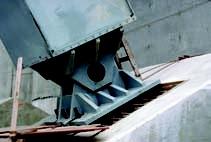
Many instructors like to present the basic theory of say, beam bending, and then use real world examples to motivate student interest in the subject of beam flexure, beam design, etc. In many cases, structures on campus offer easy access to beams, frames, and bolted connections that can be dissected in lecture or in homework problems, to find reactions at supports, forces and moments in members and stresses in connections. In addition, study of causes of failures in structures and components also offers the opportunity for students to begin the process of learning from actual designs and past engineering mistakes. A number of the new example problems and also the new and revised end-of-chapter problems in this ninth edition are based upon actual components or structures and are accompanied by photographs so that the student can see the real world problem alongside the simplified mechanics model and free-body diagrams used in its analysis.

An increasing number of universities are using rich media lecture (and/ or classroom) capture software (such as Panopto and Tegrity) in their large undergraduate courses in mathematics, physics, and engineering. The many new photos and enhanced graphics in the ninth edition are designed to support this enhanced lecture mode.

Key Features

The main topics covered in this book are the analysis and design of structural members subjected to tension, compression, torsion, and bending, including the fundamental concepts mentioned above. Other important topics are the transformations of stress and strain, combined loadings and combined stress, deflections of beams, and stability of columns. Some additional specialized topics include the following: stress concentrations, dynamic and impact loadings, non-prismatic members, shear centers, bending of beams of two materials (or composite beams), bending of unsymmetric beams, maximum stresses in beams, energy based approaches for computing deflections of beams, and statically indeterminate beams.

Each chapter begins with a Chapter Overview highlighting the major topics covered in that chapter and closes with a Chapter Summary and Review in which the key points as well as major mathematical formulas in the chapter are listed for quick review. Each chapter also opens with a photograph of a component or structure that illustrates the key concepts discussed in the chapter.

new Features

Some of the notable features of this ninth edition, which have been added as new or updated material to meet the needs of a modern course in mechanics of materials, are:

• Problem-Solving Approach—All examples in the text are presented in a new Four-Step Problem-Solving Approach which is patterned after that presented by R. Serway and J. Jewett in Principles of Physics, 5e, Cengage Learning, 2013. This new structured format helps students refine their problem-solving skills and improve their understanding of the main concepts illustrated in the example.

• Statics Review—The Statics Review section has been enhanced in Chapter 1. Section 1.2 includes four new example problems which illustrate calculation of support reactions and internal stress resultants for truss, beam, circular shaft and plane frame structures. Thirty-four end-of-chapter problems on statics provide students with two- and three-dimensional structures to be used as practice, review, and homework assignment problems of varying difficulty.

• Expanded Chapter Overview and Chapter Summary and Review sections The Chapter Overview and Chapter Summary sections have been expanded to include key equations and gures presented in each chapter. These summary sections serve as a convenient review for students of key topics and equations presented in each chapter.

• Continued emphasis on underlying fundamental concepts such as equilibrium, constitutive, and strain-displacement/ compatibility equations in problem solutions. Example problem and end-of-chapter problem solutions have been updated to emphasize an orderly process of explicitly writing out the equilibrium, constitutive and strain-displacement/ compatibility equations before attempting a solution.

• Expanded topic coverage—The following topics have been updated or have received expanded coverage: stress concentrations in axially loads bars (Sec. 2.10); torsion of noncircular shafts (Sec. 3.10); stress concentrations in bending (Sec. 5.13); transformed section analysis for composite beams (Sec. 6.3); generalized flexure formula for unsymmetric beams (Sec. 6.5); and updated code provisions for buckling of steel, aluminum and timber columns (Sec. 11.9).

• Many new example and end-of-chapter problems—More than forty new example problems have been added to the ninth edition. In addition, there are more than 400 new and revised end-of-chapter problems out of the 1440 problems presented in the ninth edition text. The end-of-chapter problems are now grouped as Introductory or Representative and are arranged in order of increasing difficulty.

• Centroids and Moments of Inertia review has moved to Appendix D to free up space for more examples and problems in earlier chapters.

Importance of e xample Problems

• Examples are presented throughout the book to illustrate the theoretical concepts and show how those concepts may be used in practical situations. All examples are presented in the Four-Step Problem-Solving Approach format so that the basic concepts as well as the key steps in setting up and solving each problem are clearly understood. New photographs have been added showing actual engineering structures or components to reinforce the tie between theory and application. Each example begins with a clear statement of the problem and then presents a simplified analytical model and the associated free-body diagrams to aid students in understanding and applying the relevant theory in engineering analysis of the system. In most cases, the examples are worked out in symbolic terms so as to better illustrate the ideas, and then numeric values of key parameters are substituted in the final part of the analysis step. In selected examples throughout the text, graphical display of results (e.g., stresses in beams) has been added to enhance the student’s understanding of the problem results.

Free-body diagram of truss model

In many cases, the problem involves the analysis of a real physical structure, such as this truss structure (Fig. 1-6) representing part of the fuselage of a model air plane. Begin by sketching the portion of the structure of interest showing members, supports, dimensions and loadings. This Conceptualization step in the analysis often leads to a free-body diagram (Fig. 1-7).

e xample 1-1
Figure 1-7
Figure 1-6

The next step is to simplify the problem, list known data and identify all unknowns, and make necessary assumptions to create a suitable model for analysis. This is the Categorize step.

Write the governing equations, then use appropriate mathematical and computational techniques to solve the equations and obtain results, either in the form of mathematical formulas or numerical values. The Analysis step leads to support reaction and member forces in the truss.

Solution:

The solution involves the following steps:

1. Conceptualize [hypothesize, sketch]: First sketch a free-body diagram of the entire truss model (Figure 1-7). Only known applied forces at C and unknown reaction forces at A and B are shown and then used in an equilibrium analysis to find the reactions.

2. Categorize [simplify, classify]: Overall equilibrium requires that the force components in x and y directions and the moment about the z axis must sum to zero; this leads to reaction force components A x , A y, and B y. The truss is statically determinate (unknowns: m 1 r 5 5 1 3 5 8, knowns: 2j 5 8) so all member forces can be obtained using the method of joints

3. Analyze [evaluate; select relevant equations, carry out mathematical solution]: First find the lengths of members AC and BC, which are needed to compute distances to lines of action of forces.

Law of sines to nd member lengths a and b: Use known angles Au , Bu , and Cu and 10 c 5 ft to find lengths a and b:

List the major steps in your analysis procedure so that it is easy to review or check at a later time.

Check that computed lengths a and b give length c by using the law of cosines: c (6.527 ft )( 8.794 ft )2 (6.527 ft)( 8.794 ft )cos(80) 10 ft 2251 28 5

4. Finalize [conclude; examine answer—does it make sense? Are units correct? How does it compare to similar problem solutions? ]: There are 2 j 5 8 equilibrium equations for the simple plane truss considered above and, using the method of joints, these are obtained by applying S F x 5 0 and S F y 5 0 at each joint in succession. A computer solution of these simultaneous equations leads to the three reaction forces and five member forces. The method of sections is an efficient way to find selected member forces.

List the major steps in the Finalize step, review the solution to make sure that it is presented in a clear fashion so that it can be easily reviewed and checked by others. Are the expressions and numerical values obtained reasonable? Do they agree with your initial expectations?

Problems

In all mechanics courses, solving problems is an important part of the learning process. This textbook offers more than 1440 problems, many with multiple parts, for homework assignments and classroom discussions. The problems are placed at the end of each chapter so that they are easy to find and don’t break up the presentation of the main subject matter. Also, problems are generally arranged in order of increasing difficulty, thus alerting students to the time necessary for solution. Answers to all problems are listed near the back of the book.

Considerable effort has been spent in checking and proofreading the text so as to eliminate errors. If you happen to find one, no matter how trivial, please notify me by e-mail (bgoodno@ce.gatech.edu). We will correct any errors in the next printing of the book.

Units

Both the International System of Units (SI) and the U.S. Customary System (USCS) are used in the examples and problems. Discussions of both systems and a table of conversion factors are given in Appendix A. For problems involving numerical solutions, odd-numbered problems are in USCS units and evennumbered problems are in SI units. This convention makes it easy to know in advance which system of units is being used in any particular problem. In addition, tables containing properties of structural-steel shapes in both USCS and SI units may be found in Appendix F so that solution of beam analysis and design examples and end-of-chapter problems can be carried out in either USCS or SI units.

Supplements

Instructor Resources

An Instructor’s Solutions Manual is available in both print and digital versions, and includes solutions to all problems from this edition with Mathcad solutions available for some problems. The Manual includes rotated stress elements for problems as well as an increased number of free body diagrams. The digital version is accessible to instructors on http://login.cengage.com. The Instructor Resource Center also contains a full set of Lecture Note PowerPoints .

Student Resources

FE Exam Review Problems has been updated and now appears online. This supplement contains 106 FE-type review problems and solutions, which cover all of the major topics presented in the text and are representative of those likely to appear on an FE exam. Each of the problems is presented in the FE Exam format and is intended to serve as a useful guide to the student in preparing for this important examination. Many students take the Fundamentals of Engineering Examination upon graduation, the first step on their path to registration as a Professional Engineer. Most of these problems are in SI units which is the system of units used

on the FE Exam itself, and require use of an engineering calculator to carry out the solution. The student must select from four available answers, only one of which is the correct answer. Go to http://www.cengagebrain.com to find the FE Exam Review Problems and the resources below, which are available on the student website for this book:

• Answers to the FE Exam Review Problems

• Detailed Solutions for Each Problem

S.P. Timoshenko (1878–1972) and J.M. Gere (1925–2008)

Many readers of this book will recognize the name of Stephen P. Timoshenko— probably the most famous name in the field of applied mechanics. A brief biography of Timoshenko appears in the first reference in the References and Historical Notes section. Timoshenko is generally recognized as the world’s most outstanding pioneer in applied mechanics. He contributed many new ideas and concepts and became famous for both his scholarship and his teaching. Through his numerous textbooks he made a profound change in the teaching of mechanics not only in this country but wherever mechanics is taught. Timoshenko was both teacher and mentor to James Gere and provided the motivation for the first edition of this text, authored by James M. Gere and published in 1972. The second and each subsequent edition of this book were written by James Gere over the course of his long and distinguished tenure as author, educator, and researcher at Stanford University. James Gere started as a doctoral student at Stanford in 1952 and retired from Stanford as a professor in 1988 having authored this and eight other well-known and respected text books on mechanics, and structural and earthquake engineering. He remained active at Stanford as Professor Emeritus until his death in January of 2008.

Acknowledgments

To acknowledge everyone who contributed to this book in some manner is clearly impossible, but I owe a major debt to my former Stanford teachers, especially my mentor and friend, and co-author James M. Gere.

I am grateful to my many colleagues teaching Mechanics of Materials at various institutions throughout the world who have provided feedback and constructive criticism about the text; for all those anonymous reviews, my thanks. With each new edition, their advice has resulted in significant improvements in both content and pedagogy.

My appreciation and thanks also go to the reviewers who provided specific comments for this ninth edition:

Erian Armanios, University of Texas at Arlington

Aaron S. Budge, Minnesota State University, Mankato

Virginia Ferguson, University of Colorado, Boulder

James Giancaspro, University of Miami

Paul Heyliger, Colorado State University

Eric Kasper, California Polytechnic State University, San Luis Obispo

Richard Kunz, Mercer University

David Lattanzi, George Mason University

Gustavo Molina, Georgia Southern University

Suzannah Sandrik, University of Wisconsin—Madison

Morteza A.M. Torkamani, University of Pittsburgh

I wish to also acknowledge my Structural Engineering and Mechanics colleagues at the Georgia Institute of Technology, many of whom provided valuable advice on various aspects of the revisions and additions leading to the current edition. It is a privilege to work with all of these educators and to learn from them in almost daily interactions and discussions about structural engineering and mechanics in the context of research and higher education. I wish to extend my thanks to my many current and former students who have helped to shape this text in its various editions. Finally, I would like to acknowledge the excellent work of Edwin Lim who suggested new problems and also carefully checked the solutions of many of the new examples and end of chapter problems.

I wish to acknowledge and thank the Global Engineering team at Cengage Learning for their dedication to this new book:

Timothy Anderson, Product Director; Mona Zeftel, Senior Content Developer; D. Jean Buttrom, Content Project Manager; Kristin Stine, Marketing Manager; Elizabeth Brown and Brittany Burden, Learning Solutions Specialists; Ashley Kaupert, Associate Media Content Developer; Teresa Versaggi and Alexander Sham, Product Assistants; and Rose Kernan of RPK Editorial Services, Inc.

They have skillfully guided every aspect of this text’s development and production to successful completion.

I am deeply appreciative of the patience and encouragement provided by my family, especially my wife, Lana, throughout this project. Finally, I am very pleased to continue this endeavor begun so many years ago by my mentor and friend, Jim Gere. This ninth edition text has now reached its 45th year of publication. I am committed to its continued excellence and welcome all comments and suggestions. Please feel free to provide me with your critical input at bgoodno@ce.gatech.edu.

MInDT AP on LI ne Co URS e

Mechanics of Materials is also available through MindTap, Cengage Learning’s digital course platform. The carefully-crafted pedagogy and exercises in this trusted textbook are made even more effective by an interactive, customizable eBook, automatically graded assessments, and a full suite of learning tools.

As an instructor using MindTap, you have at your fingertips the full text and a unique set of tools, all in an interface designed to save you time. MindTap makes it easy for instructors to build and customize their course, so you can focus on the most relevant material while also lowering costs for your students. Stay connected and informed through real-time student tracking that provides the opportunity to adjust your course as needed based on analytics of interactivity and performance. End-of-chapter quizzes and problem sets test students’ knowledge of concepts and numerics. Wrong answers in the algorithmically generated problem sets pop up custom step-by-step solutions to guide students how to solve the problems.

Step-through-tutorials help students master concepts and solve problems explained in examples.

Videos provide views of real world structures discussed in each chapter.

How does MindTap benefit instructors?

• You can build and personalize your course by integrating your own content into the MindTap Reader (like lecture notes or problem sets to download) or pull from sources such as RSS feeds, YouTube videos, websites, and more. Control what content students see with a built-in learning path that can be customized to your syllabus.

• MindTap saves you time by providing you and your students with automatically graded assignments and quizzes. These problems include immediate, specific feedback, so students know exactly where they need more practice.

• The Message Center helps you to quickly and easily contact students directly from MindTap. Messages are communicated directly to each student via the communication medium (email, social media, or even text message) designated by the student.

• StudyHub is a valuable studying tool that allows you to deliver important information and empowers your students to personalize their experience. Instructors can choose to annotate the text with notes and highlights, share content from the MindTap Reader, and create Flashcards to help their students focus and succeed.

• The Progress App lets you know exactly how your students are doing (and where they might be struggling) with live analytics. You can see overall class engagement and drill down into individual student performance, enabling you to adjust your course to maximize student success.

How does MindTap benefit your students?

• The MindTap Reader adds the abilities to have the content read aloud, to print from the reader, and to take notes and highlights while also capturing them within the linked StudyHub App.

• The MindTap Mobile App keeps students connected with alerts and notifications while also providing them with on-the-go study tools like Flashcards and quizzing, helping them manage their time efficiently.

• Flashcards are pre-populated to provide a jump start on studying, and students and instructors can also create customized cards as they move through the course.

• The Progress App allows students to monitor their individual grades, as well as their level compared to the class average. Doing so not only helps them stay on track in the course but also motivates them to do more, and ultimately to do better.

• The unique StudyHub is a powerful single-destination studying tool that empowers students to personalize their experience. They can quickly and easily access all notes and highlights marked in the MindTap Reader, locate bookmarked pages, review notes and Flashcards shared by their instructor, and create custom study guides.

A area

fA , wA area of ange; area of web

a, b, c dimensions, distances

C centroid, compressive force, constant of integration

c distance from neutral axis to outer surface of a beam

D diameter

d diameter, dimension, distance

E modulus of elasticity

E r , Et reduced modulus of elasticity; tangent modulus of elasticity

e eccentricity, dimension, distance, unit volume change (dilatation)

F force

f shear ow, shape factor for plastic bending, exibility, frequency (Hz)

fT torsional exibility of a bar

G modulus of elasticity in shear

g acceleration of gravity

H height, distance, horizontal force or reaction, horsepower

h height, dimensions

I moment of inertia (or second moment) of a plane area

I x , I y , I z moments of inertia with respect to x, y, and z axes

1 I x , 1 I y moments of inertia with respect to 1x and 1y axes (rotated axes)

I xy product of inertia with respect to xy axes

11 I xy product of inertia with respect to 11xy axes (rotated axes)

I P polar moment of inertia

1 I , 2 I principal moments of inertia

J torsion constant

K stress-concentration factor, bulk modulus of elasticity, effective length factor for a column

k spring constant, stiffness, symbol for / PEI

kT torsional stiffness of a bar

L length, distance

LE effective length of a column

ln, lognatural logarithm (base e); common logarithm (base 10)

M bending moment, couple, mass

M P , MY plastic moment for a beam; yield moment for a beam

m moment per unit length, mass per unit length

N axial force

n factor of safety, integer, revolutions per minute (rpm)

O origin of coordinates

9O center of curvature

P force, concentrated load, power

allowP allowable load (or working load)

crP critical load for a column

PP plastic load for a structure

Pr , Pt reduced-modulus load for a column; tangent-modulus load for a column

PY yield load for a structure

p pressure (force per unit area)

Q force, concentrated load, rst moment of a plane area

q intensity of distributed load (force per unit distance)

R reaction, radius

r radius, radius of gyration (/ ) rI A 5

S section modulus of the cross section of a beam, shear center

s distance, distance along a curve

T tensile force, twisting couple or torque, temperature

TP, TY plastic torque; yield torque

t thickness, time, intensity of torque (torque per unit distance)

ft , w t thickness of ange; thickness of web

U strain energy

u strain-energy density (strain energy per unit volume)

ur , ut modulus of resistance; modulus of toughness

V shear force, volume, vertical force or reaction

v de ection of a beam, velocity

9v , 0 v , etc. dv/dx, / 22dv dx , etc.

W force, weight, work

w load per unit of area (force per unit area)

x, y, z rectangular axes (origin at point O)

xc , yc , zc rectangular axes (origin at centroid C)

x , y , z coordinates of centroid

Z plastic modulus of the cross section of a beam

a angle, coef cient of thermal expansion, nondimensional ratio

b angle, nondimensional ratio, spring constant, stiffness

Rb rotational stiffness of a spring

g shear strain, weight density (weight per unit volume)

xyg , yz g , zxg shear strains in xy, yz, and zx planes

11xyg shear strain with respect to 11xy axes (rotated axes)

gu shear strain for inclined axes

d de ection of a beam, displacement, elongation of a bar or spring

∆T temperature differential

Pd , Yd plastic displacement; yield displacement

« normal strain

x« , y « , z« normal strains in x, y, and z directions

1x« , 1y « normal strains in 1x and 1y directions (rotated axes)

«u normal strain for inclined axes

1« , 2« , 3« principal normal strains

« 9 lateral strain in uniaxial stress

T« thermal strain

Y« yield strain

u angle, angle of rotation of beam axis, rate of twist of a bar in torsion (angle of twist per unit length)

pu angle to a principal plane or to a principal axis

su angle to a plane of maximum shear stress

k curvature (1/) kr 5

l distance, curvature shortening

n Poisson’s ratio

r radius, radius of curvature (1/) rk 5 , radial distance in polar coordinates, mass density (mass per unit volume)

s normal stress

x s , y s , z s normal stresses on planes perpendicular to x, y, and z axes

1x s , 1y s normal stresses on planes perpendicular to 11xy axes (rotated axes)

su normal stress on an inclined plane

1s , 2s , 3s principal normal stresses

allows allowable stress (or working stress)

cr s critical stress for a column (/ ) crcrPA s 5

pl s proportional-limit stress

r s residual stress

Ts thermal stress

Us , Ys ultimate stress; yield stress

t shear stress

xy t , yz t , zx t shear stresses on planes perpendicular to the x, y, and z axes and acting parallel to the y, z, and x axes

11xy t shear stress on a plane perpendicular to the 1x axis and acting parallel to the 1y axis (rotated axes)

tu shear stress on an inclined plane

allow t allowable stress (or working stress) in shear

Ut , Yt ultimate stress in shear; yield stress in shear

f angle, angle of twist of a bar in torsion

c angle, angle of rotation

v angular velocity, angular frequency (2 ) f vp 5

GReeK ALPHABeT

A a AlphaN n Nu

B b Beta J j Xi

Γ g GammaO o Omicron

D d Delta Π p Pi

E « EpsilonP r Rho

Z z Zeta S s Sigma

H h EtaT t Tau

Θ u Theta Y y Upsilon

I ι Iota F f Phi

K k KappaX x Chi

Λ l Lambda Ψ c Psi

M m Mu Ω v Omega

Tension, Compression, and Shear

This telecommunications tower is an assemblage of many members that act primarily in tension or compression.

Chapter Objectives

• Define mechanics of materials, which examines the stresses, strains, and displacements in structures made of various materials acted on by a variety of different loads.

• Study normal stress () s and normal strain () « in materials used for structural applications.

• Identify key properties of various materials, such as the modulus of elasticity (E) and yield y () s and ultimate u () s stresses, from plots of stress () s versus strain () «

• Plot shear stress () t versus shear strain () g and identify the shearing modulus of elasticity (G).

• Study Hooke’s Law for normal stress and strain E () s 5« and also for shear stress and strain tg 5 G ().

Chapter Outline

1.1 Introduction to Mechanics of Materials 2

1.2 Problem-Solving Approach 2

1.3 Statics Review 3

1.4 Normal Stress and Strain 22

1.5 Mechanical Properties of Materials 31

1.6 Elasticity, Plasticity, and Creep 38

• Investigate changes in lateral dimensions and volume of a bar, which depend upon Poisson’s ratio () n for the material of the bar.

• Study normal, shear, and bearing stresses in simple bolted connections between members.

• Use factors of safety to establish allowable values of stresses.

• Introduce basic concepts of design: the iterative process by which the appropriate size of structural members is determined to meet a variety of both strength and stiffness requirements.

1.7 Linear Elasticity, Hooke’s Law, and Poisson’s Ratio 44

1.8 Shear Stress and Strain 50

1.9 Allowable Stresses and Allowable Loads 63

1.10 Design For Axial Loads and Direct Shear 70 Chapter Summary and Review 74 Problems 77

Jan Jirous/Shutterstock.com

1.1 Introduction to

Mechanics of Materials

Mechanics of materials is a branch of applied mechanics that deals with the behavior of solid bodies subjected to various types of loading. Other names for this field of study are strength of materials and mechanics of deformable bodies. The solid bodies considered in this book include bars with axial loads, shafts in torsion, beams in bending, and columns in compression.

The principal objective of mechanics of materials is to determine the stresses, strains, and displacements in structures and their components due to the loads acting on them. An understanding of mechanical behavior is essential for the safe design of all types of structures, whether airplanes and antennas, buildings and bridges, machines and motors, or ships and spacecraft. That is why mechanics of materials is a basic subject in so many engineering fields. Most problems in mechanics of materials begin with an examination of the external and internal forces acting on a stable deformable body. First the loads acting on the body are defined, along with its support conditions, then reaction forces at supports and internal forces in its members or elements are determined using the basic laws of static equilibrium (provided that the body is statically determinate).

In mechanics of materials you study the stresses and strains inside real bodies, that is, bodies of finite dimensions that deform under loads. To determine the stresses and strains, use the physical properties of the materials as well as numerous theoretical laws and concepts. Mechanics of materials provides additional essential information, based on the deformations of the body, to solve statically indeterminate problems (not possible using the laws of static equilibrium alone).

Theoretical analyses and experimental results have equally important roles in mechanics of materials. Theories are used to derive formulas and equations for predicting mechanical behavior but these expressions cannot be used in practical design unless the physical properties of the materials are known. Such properties are available only after careful experiments have been carried out in the laboratory. Furthermore, not all practical problems are amenable to theoretical analysis alone, and in such cases physical testing is a necessity.

The historical development of mechanics of materials is a fascinating blend of both theory and experiment—theory has pointed the way to useful results in some instances, and experiment has done so in others. Such famous persons as Leonardo da Vinci (1452–1519) and Galileo Galilei (1564–1642) performed experiments to determine the strength of wires, bars, and beams, although they did not develop adequate theories (by today’s standards) to explain their test results. By contrast, the famous mathematician Leonhard Euler (1707–1783) developed the mathematical theory of columns and calculated the critical load of a column in 1744, long before any experimental evidence existed to show the significance of his results. Without appropriate tests to back up his theories, Euler’s results remained unused for over a hundred years, although today they are the basis for the design and analysis of most columns (see Refs. 1-1, 1-2, and 1-3).

1.2 Problem-Solving Approach*

The study of mechanics divides naturally into two parts: first, understanding the general concepts and principles, and second, applying those concepts and principles to physical situations. You can gain an understanding of the general

*The four step problem-solving approach presented here is patterned after that presented by R. Serway and J. Jewett in Principles of Physics, 5e, Cengage Learning, 2013.

concepts by studying the discussions and derivations presented in this book. You can gain skill only by solving problems on your own. Of course, these two aspects of mechanics are closely related, and many experts in mechanics will argue that you do not really understand the concepts if you cannot apply them. It is easy to recite the principles, but applying them to real situations requires an in-depth understanding. Problem solving gives meaning to the concepts and also provides an opportunity to gain experience and develop judgment.

A major objective of this text is to assist you in developing a structured solution process for problems in statics and mechanics of materials. This process is referred to as a problem-solving approach (PSA) and is used in all example problems in the text. The PSA involves the following four steps:

1. Conceptualize [hypothesize, sketch]: List all relevant data and draw a sketch showing all applied forces, support/boundary conditions, and interactions between adjacent bodies. Development and refinement of the free-body diagram is an essential part of this step.

2. Categorize [simplify, classify]: Identify the unknowns in the problem and make any necessary assumptions to simplify the problem and streamline the solution process.

3. Analyze [evaluate; select relevant equations, carry out mathematical solution]: Apply appropriate theories, set up the necessary equations for the chosen mathematical model, and then solve for the unknowns.

4. Finalize [conclude; examine answer—Does it make sense? Are units correct? How does it compare to similar problem solutions?]: Study the answers, compare them to those for similar problems you have solved in the past, and test the robustness of the solution by varying key parameters to see how the results change (perhaps even plot the main result as a function of that parameter to investigate the sensitivity of the answer).

You are encouraged to study the problem-solving approach presented in the example problems and then apply it to homework and in-class laboratory problems. This structured systematic approach also will be useful during examinations. See Appendix B.2 for further discussion of the Problem Solving Approach summarized above.

All problems appear at the ends of the chapters, with the problem numbers and subheadings identifying the sections to which they belong. In the case of problems requiring numerical solutions, odd-numbered problems are in U.S. Customary System (USCS) units and even-numbered problems are in International System of Units (SI).

In this book, final numerical results are usually presented with three significant digits when a number begins with the digits 2 through 9, and with four significant digits when a number begins with the digit 1. Intermediate values are often recorded with additional digits to avoid losing numerical accuracy due to rounding of numbers.

1.3 Statics Review

In your prerequisite course on statics, you studied the equilibrium of rigid bodies acted upon by a variety of different forces and supported or restrained in such a way that the body was stable and at rest. As a result, a properly restrained body could not undergo rigid-body motion due to the application of static forces. You drew free-body diagrams of the entire body, or of key parts of the body, and then

applied the equations of equilibrium to find external reaction forces and moments or internal forces and moments at critical points. In this section, the basic static equilibrium equations are reviewed and then applied to the solution of example structures (both two and three-dimensional) using both scalar and vector operations (both acceleration and velocity of the body are assumed to be zero). Most problems in mechanics of materials require a static analysis as the first step, so all forces acting on the system and causing its deformation are known. Once all external and internal forces of interest have been found, you can proceed with the evaluation of stresses, strains, and deformations of bars, shafts, beams, and columns as described in subsequent chapters.

Equilibrium Equations

The resultant force R and resultant moment M of all forces and moments acting on either a rigid or deformable body in equilibrium are both zero. The sum of the moments may be taken about any arbitrary point. The resulting equilibrium equations can be expressed in vector form as:

where F is one of a number of vectors of forces acting on the body and r is a position vector from the point at which moments are taken to a point along the line of application of any force F. It is often convenient to write the equilibrium equations in scalar form using a rectangular Cartesian coordinate system, either in two dimensions (x, y) or three dimensions (x, y, z) as

Equation (1-3) can be used for two-dimensional or planar problems, but in three dimensions, three force and three moment equations are required:

If the number of unknown forces is equal to the number of independent equilibrium equations, these equations are sufficient to solve for all unknown reaction or internal forces in the body, and the problem is referred to as statically determinate (provided that the body is stable). If the body or structure is constrained by additional (or redundant) supports, it is statically indeterminate, and a solution is not possible using the laws of static equilibrium alone.

Applied Forces

External loads applied to a body or structure may be either concentrated or distributed forces or moments. For example, force FB (with units of pounds, lb, or newtons, N) in Fig. 1-1 is a point or concentrated load and is assumed to act at point B on the body, while moment MA is a concentrated moment or couple (with units of lb-ft or N · m) acting at point A

Distributed forces may act along or normal to a member and may have constant intensity, such as line load 1q normal to member BC (Fig. 1-1) or line load 2 q acting in the y direction on inclined member DF ; both 1q and 2 q have units of force intensity (lb/ft or N/m). Distributed loads also

may have a linear (or other) variation with some peak intensity 0 q (as on member ED in Fig. 1-1). Surface pressures p (with units of lb/ft 2 or Pa), such as wind acting on a sign (Fig. 1-2), act over a designated region of a body. Finally, a body force w (with units of force per unit volume, lb/ft 3 or N/m 3 ), such as the distributed self-weight of the sign or post in Fig. 1-2, acts throughout the volume of the body and can be replaced by the component weight W acting at the center of gravity (c.g.) of the sign () Ws or post () W p . In fact, any distributed loading (line, surface, or body force) can be replaced by a statically equivalent force at the center of gravity (or center of pressure for wind) of the distributed loading when overall static equilibrium of the structure is evaluated using Eqs. (1-1) to (1-5).

Free-Body Diagrams

A free-body diagram (FBD) is an essential part of a static analysis of a rigid or deformable body. All forces acting on the body, or component part of the body, must be displayed on the FBD if a correct equilibrium solution is to be obtained. This includes applied forces and moments, reaction forces and moments, and any connection forces between individual components. For example, an overall FBD of the plane frame in Fig. 1-1 is shown in Fig. 1-3a; all applied and reaction forces are shown on this FBD and statically equivalent concentrated loads are displayed for all distributed loads. Statically equivalent forces 0 F q , 1 F q , and 2 F q , each acting at the c.g. of the corresponding distributed loading, are used in the equilibrium equation solution to represent distributed loads 0 q , 1q , and 2 q , respectively.

Next, the plane frame has been disassembled in Fig. 1-3b, so that separate FBDs can be drawn for each part of the frame, thereby exposing pinconnection forces at (, ) D DD xy . Both FBDs must show all applied forces as well as reaction forces Ax and A y at pin-support joint A and Fx and F y at

Figu RE 1-1

Plane frame structure

Figu RE 1-2

Wind on sign

Figu RE 1-3

(a) Overall FBD of plane frame structure from Fig. 1-1, and (b) Separate free-body diagrams of part ABCDE and part DF of the plane frame structure in Fig. 1-1

pin-support joint F. The forces transmitted between frame elements EDC and DF at pin connection D must be determined if the proper interaction of these two elements is to be accounted for in the static analysis.

The FBDs presented in Figs. 1-3a and 1-3b are essential parts of this solution process. A statics sign convention is usually employed in the solution for support reactions; forces acting in the positive directions of the coordinate axes are assumed positive, and the right-hand rule is used for moment vectors.

Reactive Forces and Support Conditions

Proper restraint of the body or structure is essential if the equilibrium equations are to be satisfied. A sufficient number and arrangement of supports must be present to prevent rigid-body motion under the action of static forces. A reaction force at a support is represented by a single arrow with a slash drawn through it (see Fig. 1-3) while a moment restraint at a support is shown as a double-headed or curved arrow with a slash. Reaction forces and moments usually result from the action of applied forces of the types described above (i.e., concentrated, distributed, surface, and body forces).

A variety of different support conditions may be assumed depending on whether the problem is 2D or 3D. Supports A and F in the 2D plane frame structure shown in Fig. 1-1 and Fig. 1-3 are pin supports, while the base of the 3D sign structure in Fig. 1-2 may be considered to be a fixed or clamped support. Some of the most commonly used idealizations for 2D and 3D supports, as well as interconnections between members or elements of a structure, are illustrated in Table 1-1. The restraining or transmitted forces and moments associated with each type of support or connection are displayed in the third column of the table (these are not FBDs, however). The reactions forces and moments for the 3D sign structure in Fig. 1-2 are shown on the FBD in Fig. 1-4a; only reactions R y , Rz , and M x are nonzero because the sign structure and wind loading are symmetric with respect to the y -z plane. If the sign is eccentric to the post (Fig. 1-4b), only reaction Rx is zero for the case of wind loading in the z direction. (See Problems 1.8-19 and 1.9-17 at the end of Chapter 1 for a more detailed examination of the reaction forces due to wind pressure acting on several sign structures similar to that shown in Fig. 1-2; forces and stresses in the base plate bolts are also computed).

Figu RE 1-4

(a) FBD of symmetric sign structure, and (b) FBD of eccentric sign structure

Table 1-1

Modeling reaction forces and support conditions in 2D or 3D static analysis

Type of support or connection

Simplified sketch of support or connection

Display of restraint forces and moments, or connection forces

1. Roller Support: A single reaction force R is developed and is normal to the rolling surface; force R opposes motion into or away from the rolling surface. The rolling surface may be horizontal, vertical, or inclined at some angle u. If friction is present, then include a force F opposing the movement of the support and tangential to the rolling surface. In 3D, the roller moves in the x-z plane and reaction R y is normal to that plane.

Bridge with roller support (see 1.1, 1.2)

(1.1) (1.2) (1.3)

Horizontal roller support [(1.1), (1.2)]; or alternate representation as rocker support [(1.3)]

Both downward and uplift motions are restrained.

(a) Two-dimensional roller support (friction force F 5 0 for smooth rolling surface)

Vertical roller restraints

Bridge with rocker support (see 1.3)

Rotated or inclined roller support

(b) Three-dimensional roller support (friction force F 5 0 for smooth rolling surface; reaction R y acts normal to plane x-z on which roller translates)

3D roller support

2. Pin Support: A single resultant force, usually shown using two rectangular components Rx and R y in 2D but three components in 3D, resists motion in any direction normal to the pin. The pin support cannot resist moment, and the pin is free to rotate about the z axis. In 3D, the pin becomes a balland-socket joint or support.

Two-dimensional pin

(a) Two-dimensional pin support x

Ball-and-socket joint model (camera mount, 3D)

(b) Three-dimensional pin support

Ball-and-socket joint model

Hip prosthesis for hip replacement

3. Sliding Support: A support that translates without rotation is a sliding support. Examples are a collar sliding along a sleeve or a flange moving within a slot. Reactions in 2D are a force Rx normal to the sleeve and a moment Mz representing resistance to rotation relative to the sleeve. In 3D, the sliding support translates on frictionless plane y-z and reaction moment components M y and Mz prevent rotation relative to that plane.

(a) Two-dimensional sliding support (support translates on frictionless path along 1y or y direction)

Frictionless sleeve on vertical shaft

Sliding support for column light stand

Two-dimensional sliding support

Friction F opposes motion in 1y direction in 2D along sliding surface; F is zero if smooth surface is assumed.

In 3D, add restraint moment M x to prevent rotation about x axis.

(b) Three-dimensional sliding support (support translates on frictionless y-z plane)

© David Chapman/Alamy Stock

Turn static files into dynamic content formats.

Create a flipbook
Issuu converts static files into: digital portfolios, online yearbooks, online catalogs, digital photo albums and more. Sign up and create your flipbook.