Process Control Modeling Design And Simulation 1st Edition Bequette Solutions Manual

Table of Contents

Solutions for Chapters 1-14

Solutions for Module 5.4 and Module 5.5

Solution for Module 16, Discrete PI Example

Chapter1Solutions

1.1

i Drivingacar

Pleaseseeeitherjogging,cycling,stirredtank heater,orhouseholdthermostatforarepresentativeanswer.

ii Twosamplefavoriteactivities: Jogging

(a) Objectives:

• Jogintensely(heartrateat180bpm) for30min.

• Smoothchangesinjoggingintensity andspeed.

(b) InputVariables:

• JoggingRate–Manipulatedinput

• Shockingsurprises(dogs,cars,etc.)–Disturbance

(c) OutputVariables:

• BloodOxygenlevel–unmeasured

• Heartbeat–measured

• Breathingrate–unmeasured

(d) Constraints:

• Hard:MaxHeartRate(toavoidheart attack → death)

• Hard:Bloodoxygenminimumand maximum

• Soft:Timespentjogging

(e) Operatingcharacteristics:Continuousduringperiod,SemiBatchwhenviewedover largertimeperiods.

(f) Safety,environmental,economicfactors: Potentialforinjury,overexertion

(g) Control:Feedback/Feedforwardsystem. Oxygenlevel,heartbeat,fatigueallpartof determiningactionafterthefact.Path, weatherarepartoffeedforwardsystem

Cycling

(a) Objectives:

• Ensurestability(don’tcrash)

• Enjoyride

• Preventmechanicalfailure

(b) InputVariables–Manipulated:

• BodyPosition

• Steering

• BrakingForce

• GearSelection

InputVariables–Disturbances:

• Weather

• PathConditions

• Otherpeople,animals

(c) OutputVariables–Measured:

• Speed

• Direction

• CaloricOutput(viaelectronicmonitor)

OutputVariables–Unmeasured:

• Levelofenjoyment

• Mechanicalintegrityofpersonandbicycle

• Aesthetics(smoothnessofride)

(d) Constraints–Hard:

• Turningradius

• Mechanicallimitsofbikeandperson

• Maximumfatiguelimitofperson

Constraints–Soft:

• Steeringdynamicsthatleadtoinstabilitybeforemechanicalfailure(i.e.you crash,thebikedoesn’tbreak)

• Terrainandweathercanlimitenjoymentlevel.

(e) Operation:Continuous:Steering,weight distribution,terrainselectionwithinapath, pedalforceSemibatch:Gearselection, brakingforceBatch:Tirepressure,bikeselection,pathselection

(f) Safety,environment,economics:Safety: StabilityandmechanicallimitspreventinjurytoriderandothersEnvironment:Trail erosion,noiseEconomics:Healthcosts, maintenancecosts

(g) ControlStructure:Feedback:Levelsofexertion,bikeperformancearemonitoredand rideisadjustedafterthefactFeedForward: Pathisseenaheadandrideisadjustedaccordingly.

iii Astirredtankheater

(a) Objectives

• MaintainOperatingTemperature

• Maintainflowrateatdesiredlevel

(b) InputVariables: 1-1

• Manipulated:Addedheattosystem

• Disturbance:Upstreamflowrateand conditions

(c) OutputVariables–Measured:Tankfluid temperature,Outflow

(d) Constraints:

• Hard:Maxinflowandoutflowasper pipesizeandvalvelimitations

• Soft:Fluidtemperatureforoperating objective

(e) Operatingconditions:Continuousfluid flowadjustment,continuousheatingadjustment

(f) Safety,Environmental,Economicconsiderations:Safety:Tankoverflow,failurecould causeinjuryEconomics:Heatingcosts,spill costs,processqualitycostsEnvironmental: Energyconsumption,contaminationdueto spillsofhotwater

(g) ControlSystem:Feedback:Temperatureis monitored,heatingrateisadjustedFeedforward:Upstreamflowvelocityisusedto predictfuturetankstateandinputisadjustedaccordingly.

iv. Beerfermentation

Pleaseseeeitherjogging,cycling,stirredtank heater,orhouseholdthermostatforarepresentativeanswer.

v. Anactivatedsludgeprocess

Pleaseseeeitherjogging,cycling,stirredtank heater,orhouseholdthermostatforarepresentativeanswer.

vi. Ahouseholdthermostat

(a) Objectives:

• Maintaincomfortabletemperature

• Minimizeenergyconsumption

(b) InputVariables:

• Manipulated:Temperaturesetting

• Disturbance:Outsidetemperature,energytransmissionbetweenhouseand environment

(c) OutputVariables:

• Measured:Thermostatreading

• Unmeasured:Comfortlevel

(d) Constraints:

• Hard:Maxheatingorcoolingdutyof system

• Soft:Maxorminimumtemperaturefor comfort

(e) Operatingconditions:Continuousheating adjustment,continuoustemperaturereading.

(f) Safety,Environmental,Economicconsiderations:Safety:heatermaybeanelectricalorburninghazardEconomics:Heating costsEnvironmental:Energyconsumption.

(g) ControlSystem:Feedback;temperatureis monitored,heatingrateisadjustedafter thefact.

vii Airtrafficcontrol

Pleaseseeeitherjogging,cycling,stirredtank heater,orhouseholdthermostatforarepresentativeanswer.

1.2

a. FluidizedCatalyticCrackingUnit

i. Summaryofpaper:

Afluidizedcatalyticcrackingunit(FCCU)is oneofthetypicalandcomplexprocessesin petroleumrefining.Itsprincipalcomponentsare areactorandagenerator.Thereactorexecutes catalyticcrackingtoproducelighterpetro-oil products.Theregeneratorrechargesthecatalystandfeedsitbacktothereactor.Inthis paper,theauthorstesttheircontrolschemeson aFCCUmodel.Themodelisanonlinearmultiinput/multi-output(MIMO)whichcouplestime varyingandstochasticprocesses.Considerable computationisneededtousemodelpredictiveprocesscontrolalgorithms(MPC).StandardPIDcontrolgivesinferiorperformance.A simplifiedMPCalgorithmisabletoreducethe numberofparametersandcomputationalload whilestillperformingbetterthanaPIDcontrol method.

ii FamiliarTerms:Constraint,nonlinearity,controlperformance,MPC,unmeasureddisturbancerejection,modeling,simulation.

b. ReactiveIonEtching PleaseseeFCCUforarepresentativeanswer.

c. RotaryLimeKiln PleaseseeFCCUforarepresentativeanswer.

d. ContinuousDrugInfusion PleaseseeFCCUforarepresentativeanswer.

1-2

e. AnaerobicDigester PleaseseeFCCUforarepresentativeanswer.

f. Distillation PleaseseeFCCUforarepresentativeanswer.

g. PolymerizationReactor PleaseseeFCCUforarepresentativeanswer.

h. pH PleaseseeFCCUforarepresentativeanswer.

i. BeerProduction PleaseseeFCCUforarepresentativeanswer.

j. PaperMachineHeadbox PleaseseeFCCUforarepresentativeanswer.

k. BatchChemicalReactor PleaseseeFCCUforarepresentativeanswer.

1.3

a. Vortex–sheddingflowmeters

Theprincipalofvortexsheddingcanbeseeninthe curlingmotionofaflagwavinginthebreeze,orthe eddiescreatedbyafastmovingstream.Theflag outlinestheshapeofairvorticesastheflowpastthe pole.VanKarmanproducedaformuladescribingthe phenomenain1911.Inthelate1960’sthefirstvortex sheddingmetersappearedonthemarket.Turbulent flowcausesvortexformationinafluid.Thefrequency ofvortexdetachmentisdirectlyproportionaltofluid velocityinmoderatetohighflowregions.Atlow velocity,algorithmsexisttoaccountfornonlinearity. Vortexfrequencyisaninput,fluidvelocityisanoutput.

b. Orifice–plateflowmeters

Pleaseseevortex–sheddingflowmetersforarepresentativeanswer.

c. Massflowmeters

Pleaseseevortex–sheddingflowmetersforarepresentativeanswer.

d. Thermocouplebasedtemperaturemeasurements

Pleaseseevortex–sheddingflowmetersforarepresentativeanswer.

e. Differentialpressuremeasurements

Pleaseseevortex–sheddingflowmetersforarepresentativeanswer.

f. Controlvalves

Pleaseseevortex–sheddingflowmetersforarepre-

sentativeanswer.

g. pH Pleaseseevortex–sheddingflowmetersforarepresentativeanswer.

1.4

NosolutionsarerequiredtoworkthroughModule1

1.5

a.

Themainobjectiveistomaintaintheprocessfluid outlettemperatureatadesiredsetpointof300C.

b.

Themeasuredoutputistheprocessfluidoutlettemperature.

c. Themanipulatedinputisthefuelgasflowrate,specificallythevalvepositionofthefuelgascontrolvalve.

d.

Possibledisturbancesinclude:processfluidflowrate, processfluidinlettemperature,fuelgasquality,and fuelgasupstreampressure.

e. Thisisacontinuousprocess.

f. Thisisafeedbackcontroller.

g.

Thecontrolvalveshouldbe fail-closed.Increasing airpressuretothevalvewillthenincreasethevalve positionandleadtoanincreaseinflowrate.Lossof airtothevalvewillcauseittoclose.Thegainofthe valveispositive,becauseanincreaseinthesignalto thevalveresultsinanincreaseinflow.

h.

Itisimportantfromasafetyperspectivetohavea fail-closedvalve.ifthevalvefailedopen,theremight notbeenoughcombustionair,causingalossofthe flame-thiscouldcausethefurnacefireboxtofillwith fuelgas,whichcouldthenre-igniteundercertainconditions.Althoughthecombustionairisnotshown,it shouldbesuppliedwithasmallstoichiometricexcess. Ifthereistoomuchexcesscombustionair,energyis wastedinheatingupairthatisnotcombusted.If thereistoolittleexcessair,combustionwillnotbe complete,causingfuelgastobewastedandpollutiontotheatmosphere.Theprocessfluidisflowing 1-3

toanotherunit.Iftheprocessfluidisnotatthe desiredsetpointtemperature,theperformanceofthe unit(reactor,etc)maynotbeasgoodasdesired,and thereforenotasprofitable.

i.

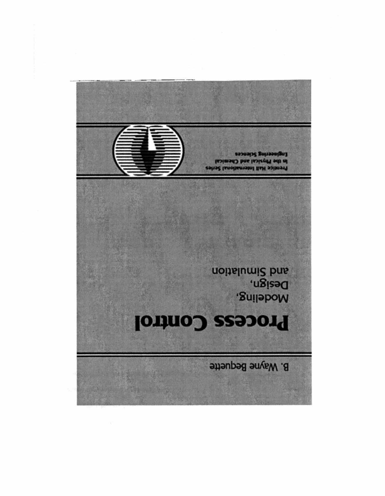
Thecontrolblockdiagramfortheprocessfurnaceis shownbelowinFigure1.Wherethethesignalsas

1.8

Weknowfromtheproblemstatementthattheinlet (Fin)andoutlet(Fout)flowratescanberepresented withthefollowingequations:

Fin =50+10sin(0.1t)

Fout =50

Thechangeinvolumeasafunctionoftimeis dV dt = Fin Fout

substitutingwhatweknow:

dV

dt =50+10sin(0.1t) 50

Figure1-1:Controlblockdiagramofprocessfurnace

follows:

• Tsp:Temperaturesetpoint

• pv :Valvetoppressure

• Fg :Fuelgasflowrate

• Fp:Processfluidflowrate

• Tp:Processfluidinlettemperature

• T:Temperatureofprocessfluidoutlet

• Tm:Measuredtemperature

1.6

Theproblemstatementtellsusthatthegasolineis worth$500,000aday.A2%increaseinvalueis:

$500, 000 day x 0.02= $10, 000 day

Wearealsogiventhattherevampwillcost $2,000,000.Wecannowcalculatethetimerequired topaybackthecontrolsysteminvestment.

$2, 000, 000 $10,000 days =200days

Therefore,weknowitwilltake200daystopayoff theinvestment.

1.7 2yrs · 4 4million$/yr · 0 2%=$176, 000

Simplifying dV dt =10sin(0 1t)

Rearrangingtheequation

dV =10sin(0 1t)dt

Takingtheintegralofbothsides

dV = 10sin(0 1t)dt

Usingbasiccalculustosolve

V V0 = 10 0 1 cos(0 1t)|t t=0

Weknowtheinitialtankvolumeis500liters

V 500= 100cos(0 1t) 100cos(0)

V 500= 100cos(0 1t)+100

V (t)=600 100cos(0 1t)

Theequationabovetellsushowthevolumeofthe tankwillvarywithtime.ThiscanalsobeseenvisuallyinFigure2below.

1.9 a.

Theobjectiveistomaintainadesiredbloodglucose concentrationbyinsulininjection.Insulinisthemanipulatedinputandbloodglucoseisthemeasured output.Asperformedbyinjection,theinputisreallydiscreteandnotcontinuous.Also,glucoseis notcontinuouslymeasured,sothemeasuredoutput isdiscrete.Disturbancesincludemealconsumption andexercise.Feedforwardactionisusedwhenadiabeticadministersaninjectiontocompensatefora

1-4

Figure1-2:Liquidvolumeasafunctionoftime

meal.Feedbackactionoccurswhenadiabeticadministersmoreorlessinsulinbasedonabloodglucose measurement.Itisimportantnottoadministertoo muchinsulin,becausethiscouldleadtotoolowofa bloodglucoselevel,resultinginhypoglycemia.

b.

Aprocessandinstrumentationdiagramofanautomatedclosed-loopsystemisshowninFigure3below. Forsimplicity,thisisshownasapumpandvalve

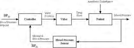
Figure1-4:controlblockdiagramofclosed-loopinsulininfusion

gainispositive.A fail-closed valveshouldbespecified.Ifthevalvefailed-open,thecoldstreamoutlet temperaturecouldbecometoohigh.

b.

Anincreaseinthehotby-passflowleadstoadecrease inthecoldstreamoutlettemperature,sothegainis negative.A fail-open valveshouldbespecified.

c.

Anincreaseinthecoldby-passflowrateleadstoa decreaseintheoutlettemperature,sothegainisnegative.A fail-open valveshouldbespecified,sothat theoutlettemperatureisnottoohighortheairpressureislost.

d. Strategy(c),coldby-pass,willhavethefastestdynamicbehaviorbecausetheeffectofchangingthebypassflowwillbealmostinstantaneous.Theother strategieshaveadynamiclagthroughtheheatexchanger.

1.11

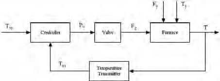
Theanesthesiologistattemptstomaintainadesired setpointforbloodpressure.Thisisdonebymanipulatingthedrugflowrate.Amajordisturbanceisthe effectofananestheticonbloodpressure.

Thecontrolblockdiagramfortheautomatedsystem isshowbelowinFigure5,where,forsimplicity,the drugisshownbeingchangedbyavalve.

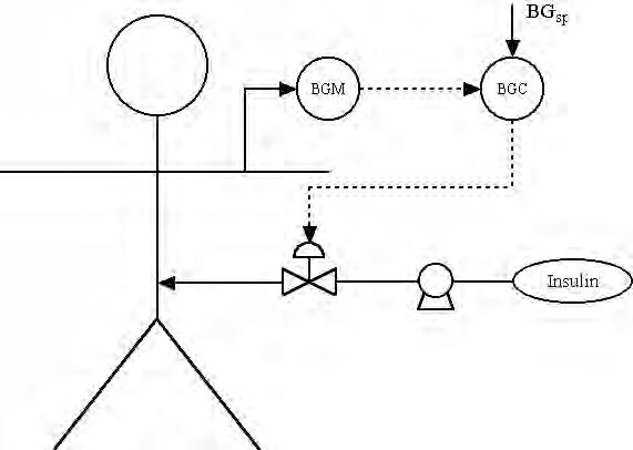
Figure1-3:P&IDofclosed-loopinsulininfusion

arrangement.Inpractice,thepumpspeedwould bevaried.Theassociatedcontrolblockdiagramis showninFigure4below.

1.10

a.

Anincreaseinthehotstreamflowrateleadstoanincreaseinthecoldstreamoutlettemperature,sothe

Figure1-5:Controlblockdiagramofdrugdelivery

Chapter2Solutions

2.1

Themodelingequationis dP dt = RT V qi RT V β P Ph

Atsteadystate

dt = RT V qi RT V β P Ph =0

V β Ps Phs = RT V qis

s = Phs + q 2 is β 2

Thuswecanconcludethatitisaself–regulatingsystem,asforachangeininputitwillattainanew steady–state.

Thesketchofthesteady–stateinput–outputcurve shouldlooklikefigure2-1.

theinletandoutletflowratesarethesame.Thus Fi V (Ti T )+ Q =0 100 500 (20 40)+ Q =0 Q =4◦ C/min

b.Forthispartweneedtointegrate dT dt = 100 500 (22 T )+4

fromaninitialstateof T =40◦ C.TheEuler formulais

xk +1 = xk +∆txk

xk = f (xk )

where f ( )istherighthandsideofthedifferentialequation,and x isthestate,inthiscase T Using∆t =0 5,andforatotalof2minutes,we have

2.2

a.Atsteady–state,thevolumewillnotchange,as

Figure2-2showsthecurveofthesolutionfound using matlab’s ode45,withthecirclesmarking thepointsoftheEulersolution.

Figure2-1:Plotfor2.1

Figure2-2:Plotfor2.2

2.3

Sincethemodelequationshaveonlytwostates, Vl and P ,wehavetoassumethefollowingareconstant: densityoftheliquid(ρ),temperature(T ),theideal gasconstant(R)andthemolecularweightofthegas (MW ).

Startingwiththebalanceoftheliquidmassinthe system,wehave

dMl dt = dVl ρ dt = Ff ρ Fρ

dVl dt = Ff F

Forthebalanceofthemassofgas

dnMW dt = qi MWi qMW

dn

dt = qi q

Fromtheidealgaslaw PVg = nRT ,wherethevolumeofgasis Vg = V Vl Then,

d(PVg )

dt = nRT dt

P d(V Vl ) dt +(V Vl ) dP dt = RT dn dt

andusingthepreviouslyderivedexpressionsfor dn dt and Vl dt

P d(V Vl ) dt +(V Vl ) dP dt = RT dn dt

P dVl dt +(V Vl ) dP dt = RT (qi q ) dP dt = P V Vl (Ff F )+ RT V Vl (qi q )

Thusourmodelequationsare

dVl dt = Ff F

2.4

solvingatsteady–state,weget

CP 1s = CAis Fs kV +1

Weneedtomeetayearlyproduction,soourfinal constraintis

Fs CP 1s S =100x106 lb/yr

Where S =62lb/lbmol 504000min/yrisourconversionfactor,assuming350daysofoperationinayear. Then,

Fs CAis Fs kV +1 S =100x106 lb/yr

solvingfortheflowrate,weget Fs =7.9256ft3 /min.

Nowweneedtoconsiderthesecondreactorinseries,whichwillalsochangetheflowrateneededto meetproductionlevels.Theequationsforthesecond reactorare dC

Solvingatsteady–state,weget

Again,weneedtomeetproductionlevels,so

Solvingfortheflowrate,weget Fs =6 5799ft3 /min. Thuswehaveasavingsof16 98%usingthetworeactorsinseriesoverasingleone.

dP

dt = P V Vl (Ff F )+ RT V Vl (qi q )

Sincewehavealargervolumethantheexample,we havetocalculatetheflowrateforasinglereactoras well.Ourvolumeis V =106.9444ft3 .Theequations forthefirsttankare

2.5

Theresultinggraphshouldbethesameasfigure2-5, exceptthatthetimerangefrom-1to0willnotappear.

Weneedequationswhosestatesare V and CA ,then

d(VCa ) dt = Fin CAin kVCA

V dCa dt + CA d(V ) dt = Fin CAin kVCA

V dCa dt = CA d(V ) dt + Fin CAin kVCA

V dCa dt = CA Fin + Fin CAin kVCA

dCa dt = Fin V (CAin CA ) kCA

ourtwoequationsare dV dt = Fin dCa dt = Fin V (CAin CA ) kCA

2.7

a.Themodelingequationsare dCw 1 dt = F V1 (Cwi Cw 1 ) kC 2 w 1 dCw 2 dt = F V2 (Cw 1 Cw 2 ) kC 2 w 2

b.Atsteady–statewecansolvethefollowingequations

Rearrangingthefirstequation,wehavethe quadratic

=0

thepositiverootgivesus Cw 1s =0 33333mol/liter

Rearrangingthesecondequation,wehavethe quadratic kC 2 w 2s + Fs V2 Cw 2s Fs V2 Cw 1s =0

thepositiverootgivesus Cw 2s =0 0900521mol/liter

c.Tolinearize,wehavethefunctions

f1 = dCw 1 dt = F V1 (Cwi Cw 1 ) kC 2 w 1

f2 = dCw 2 dt = F V2 (Cw 1 Cw 2 ) kC 2 w 2

d.Evaluatingthesecoefficientsatoursteady–state, wehave

e.Since y = x,itisstraightforwardtoshowthat

= 10 01 D = 00 00

f.Using matlab,theeigenvaluesare 0.320156 and 1.25.

andusingthestateandinputvariablesasdefined,wehave

analytically,wehave

g.Figure2-3showstheplotforthelinearandnonlinearresponses;asitcanbeseen,theextraction

UA =183 9Btu/(◦ F min)

Fjs =1 5ft3 /min

b.Applyingtheequationsfortheelementsofthe linearizationmatrices

a11 a12 a21 a22 = 0 40 3 1.2 1.8

B = 0 7.50.10 20000.6

C = 10 01

D = 0000 0000

c heater.m fileshouldbeliketheexampleinthe book(p.73)

d.Using delJ=0,run ode45 tosolvetheequationsdefinedin heater.m,thenplotthetwo statesvs.time.Theresultshouldbeconstant valuesthatmatchthesteadystatesforalltime.

h.Iftheorderofthereactionvesselsisreversed, thesteady–stateequationswehavetosolveare

e.Togetthedesiredplotsforthetwostepresponses,them–fileshowninpages74-75can beused,startingwiththedefinitionofthestate spacelinearmodel.Sincethemodelislinear, theoutputofthestepresponsecommandcanbe scaledaccordinglyforstepsofdifferentsizesby justmultiplyingby delFj.Figures4(a)and4(b) showtheresponsesforasmall(0.2%changein Fj )andalarge(10%changein Fj )steps,respectively.

f.Sinceweknow UA forthesmallvessel,andwe areassumingthat U remainsconstant,wecan findthevalueof UA foralargervolumeas

UAsmall · Alarge Asmall = UAlarge

2.8

a.Solvethefollowingtwosimultaneousequations usingtheparametersandsteady–statevalues provided:

Modelingthevesselasacylinder,thevolumeis V = π 2 D 3 ,andtheareais A =2.25πD 2 .Wecan thencalculatetheareaofthesmallvesselasa functionofitsvolume,forwhichweget

2 3

Asmall =2.25π 20 π

Similarly,wehavetheareaofthelargervesselin termsofitsvolume

Alarge =2 25π

Figure2-3:Plotfor2.7g

Applyingthis,wefindthat

Wecanalreadyseethatthesteady–statejacket temperaturehasgoneup,sowewanttoknow howlargewecanmakethevesselbeforethe jackettemperatureapproachestheinletjacket temperature.Wecansolvethefollowingequation,using Fs V =0 1min 1 ,aswewanttomaintaintheresidencetime.Wealsousetheexpressionintermsofthevolumethatwefoundin part f

then V =270ft3

h.Applyingtheequationsfortheelementsofthe linearizationmatricesusingthesteadystatefor thelargervessel,wehave

Theeigenvaluesforthesystemwiththelarge vesselareat λ1 = 0.1957and λ2 = 2.0197. Whileforthesystemwiththesmallervessel, theyare λ1 = 0.1780and λ2 = 2.0220.They areveryclosetoeachother,thusthespeedof theresponsewillbesimilarforbothvessels.

i.Figure2-5showstheresponsetoastepof 0 1ft3 /min.Comparingthistofigure4(a),we canseethatbothlinearmodelresponsesare practicallythesameasthenonlinearmodelresponse.Thechangeintemperaturesisalsominor,asthechangeinjacketflowrateissmall (0.2%ofthesteadystatevalueinbothcases).

j.Figure2-6showstheresponsetoastepof10%of thesteadystatejacketflowrate.Comparingthis tofigure4(b),wecanseethatbothlinearmodel

Figure2-4:Plotfor2.8e(a)smallstepof0.2%(b) largestepof10%

responsesareclosetothenonlinearmodelresponse,butthereisanoffsetinthesteadystate. Thechangeintemperaturesisalsomoremarked, andlargerinthecaseofthesmallerreactor,as wouldbeexpectedduetothesmallervolume.

Figure2-5:Plotfor2.8i

Figure2-6:Plotfor2.8j

Chapter4Solutions

4.1

Themaximumrate-of-changemeanstakingaderivative.Theoutputis:

y (t)= kp ∆u{1 exp( t θ τp )}

Thederivativewithrespecttotimeis:

dy dt = kp ∆u τp exp( t θ τp )

Duetothenegativesign,thelargestthatexp {− t θ τp } canbeis1.Anexponentialwillgiveavalueof1when theargumentis0.Thatmeansthefollowingistrue:

t θ τp =0

Solvingfor θ gives t = θ

Tofindthemaximumslope,plug t = θ intotheslope equation:

dy dt = kp ∆u τp exp( θ θ τp )

Whichsimplifiesdowntoamaximumslopeof:

dy dt = kp ∆u τp

4.2

Theoutputresponse y (t)forafirstorderplusdead time(FOPDT)modeltoastepchangeis:

y (t)= kp ∆u{1 exp( t θ τp )}

Recognizingthat∆y = kp ∆u gives:

y (t)=∆y {1 exp( t θ τp )}

Substituting t1 = τp 3 + θ intotheoutputequation:

y (t)=∆y {1 exp(

Cancellingouttermsgives:

Whichsimplifiesdownto:

y (t1 )=0.238∆y

Substituting t2 = τp + θ intotheoutputequation:

y (t)=∆y {1 exp( τp + θ θ τp )}

Cancellingouttermsgives:

y (t)=∆y {1 exp( 1)}

Whichsimplifiesdownto:

y (t1 )=0 632∆y

Usetheequationsfor t1 and t2 tosolvefor θ and τp

Solvingfor θ inthe

Pluggingthatintothe t1 equation:

Solvingfor τp yields:

4.3

Thefirsttechniquetoestimatetheparametersina firstorderplusdeadtime(FOPDT)modelisthe 63.2%method.Findthegainusingtheformula:

τp 3 + θ θ τp )}

y (t)=∆y {1 exp( 1 3 )}

Thetimedelaycanbe“eyeballed”bylookingat whentheoutputbeginstochangesignificantly,and whentheinputchangewasapplied.Forthisprocess:

θ =5min 1min=4min

Thetimeconstantisestimatedusingthe63.2% method.First,calculatewhat63.2%oftheoutput changeis:

Process Control Modeling

Design And Simulation 1st Edition Bequette Solutions Manual Full Download: http://testbanktip.com/download/process-control-modeling-design-and-simulation-1st-edition-bequette-solutions-manual/

Lookingattheoutputresponse,thetimefortheresponsetoreach11.376 ◦ Cis15minutes.Thetime constantcanthenbecalculatedusingtheformula giveninthechapter.

t63 2% = τ + θ

τ = t63 2% θ =15 4=11min

TheFOPDTcanthenbeexpressedas:

gp (s)= 6e 4s 10s +1

Thesecondtechniquetoestimatetheparametersin afirstorderplusdeadtime(FOPDT)modelisthe MaximumSlopemethod.Findthegainusingthe

Thetimedelaycanbe“eyeballed”bylookingat whentheoutputbeginstochangesignificantly,and whentheinputchangewasapplied.Forthisprocess:

θ =5min 1min=4min

Thetimeconstantcanbeestimatedbyfirstdeterminingwhat63.2%and28.3%oftheoutputis.

0.632∆y =(0.632)(18)=11.376

0.283∆y =(0.283)(18)=5.094

Lookingattheresponse,therespectivetimestoreach thoseoutputvaluesare t63 2 =15and t28 3 =8. Thetimeconstantcanthenbecalculatedusingthe formula:

τp =1.5(t63 2 t28 3 )

τp =1.5(15 8)=10.5min

TheFOPDTcanthenbeexpressedas:

kp = 68 50 ◦ C 28 25psig =6 ◦ C psig

Thetimedelaycanbe“eyeballed”bylookingat whentheoutputbeginstochangesignificantly,and whentheinputchangewasapplied.Forthisprocess:

θ =5min 1min=4min

Thetimeconstantcanbeestimatedusingthemaximumslopeoftheoutputresponse.Lookingatthe response,wecanseethatthemaximumslopecanbe

gp (s)= 6e 4s 10 5s +1

Notethatallthreemethodsgivesimilar,butnotidenticalFOPDTmodels.

4.4

Anintegratorplusdeadtimemodelhastheform:

gp (s)= kp e θs s

Thetimeconstantcannowbecalculatedusing:

Wethereforeneedtoestimateagainandatimedelay. Thetimedelayisestimatedbylookingatwhenthe outputbeginstochangesignificantly,andsubtracting thetimewhentheinputchangewasmade.Forthis process:

θ =3min 1min=2min

Togetthegain,weneedtofindboththeslopeof theoutputandthechangeininput.Lookingatthe figure,weseethat:

∆u =9 5 10 0lps= 0 5lps

TheFOPDTcanthenbeexpressedas:

slope = 0 3 1m 10 3min = 0 1 m min

Wecanthencalculatethegainusingtheformula:

Thesecondtechniquetoestimatetheparametersin afirstorderplusdeadtime(FOPDT)modelisthe TwoPointmethod.Findthegainusingtheformula:

kp = slope ∆u

kp = 0.1 m min 0.5lps =0 2 m min lps

Theintegratorplusdeadtimemodelisthus: