Politecnico di Torino Design for Climate Resilience Water Engineering & Architectural Technology
Submitted by:
S337635 - Hamed Kalantari
S344137 - Tamanna Kewlani
S274818 - Zheng Zhou
S350946 - Eugenia Chapellin
S358807 - Federica Lo Cascio
S344898 - Rumeysa Arslankurt
January 19, 2026
CLIMATE RESILIENCE ANALYSIS FOR CAPE
TOWN - ACADEMIC REPORT #1
Executive Summary
This report provides a comprehensive, academically oriented analysis of climate resilience factors for the city of Cape Town. It expands five diagnostic exercises into detailed, step by step methodologies, complete with formulas, assumptions, calculations, and interpretation.
Introduction and Objectives
Coastal cities such as Cape Town face interlinked climate challenges: elevated solar radiation and surface heat loads, increasing frequency of extreme rainfall events, and the requirement to align local measures with national greenhouse gas reduction commitments. Over the past decade, Cape Town’s climate has become increasingly unpredictable, revealing the extent to which the city is vulnerable to the accelerating impacts of global climate change. On a national scale, South Africa has recognized the urgency of these environmental changes and developed a framework for addressing them. The country’s Nationally Determined Contribution (NDC) outlines commitments to improve overall resilience and cities like Cape Town play a crucial role, as urban areas are major contributors to energy consumption and emissions.
This report aims to translate diagnostic outputs into operational metrics and design targets. The exercises address:
1. Net Radiation Estimation (Rn),
2. Emissions and NDC Alignment,
3. Surface Urban Heat Island (SUHI) and Tree Cover,
4. Integrated Flood and Heatwave Risk,
5 Urban Greening Factor (UGF)
Data Sources and Common Assumptions
Primary inputs were provided by the project dataset (EX1–EX3) Supplementary reference sources include Global Solar Atlas (DNI), national NDC documentation, Our World in Data, and remote sensing products (Landsat, Sentinel-2, Yale UHI Explorer).
Common unit conversions and assumptions are documented in each exercise but include: converting kWh/m²/year to average W/m² using a 365-day year; using empirically derived conversion factors where needed; and reporting uncertainties when assumptions require approximations.
1. NET RADIATION ESTIMATION (Rn)
Net radiation (Rn) is a key component of the surface energy balance and is closely linked to surface temperature and urban heat loads. Rn is commonly derived from measured or modeled shortwave radiation and longwave components. In this exercise our objective is to build a picture of our assigned country's expected future climate by determining the current Rn for three representative cities and collecting their historical and projected temperature time series for various scenarios (RCPs/SSPs).
1.1. Theory and Formula
The empirical relationship used in the supplied materials (Jiang et al., 2015, as referenced) is: Rn = 0.654 × Snet − 20.3
Where Rn is net radiation in W/m² and Snet is the net shortwave irradiation W/m². This relation provides a first-order estimate of Rn from Snet and is suitable for comparative diagnostic analyses.
1.2. Step-by-Step Calculation Method
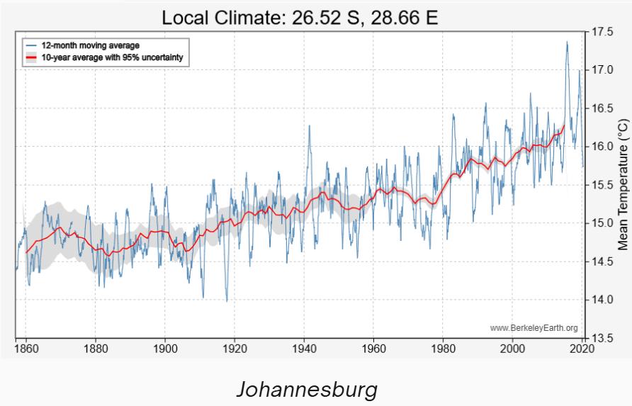
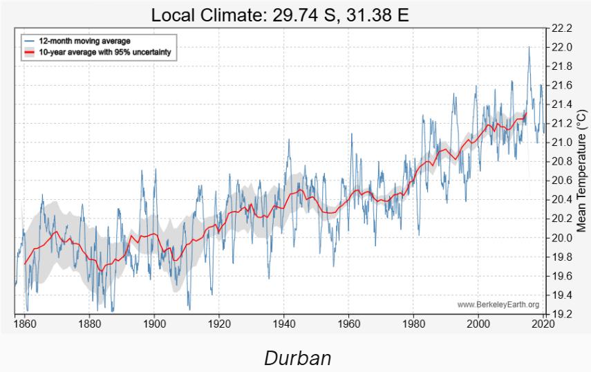
For this exercise we have chosen the cities of Cape Town, Johannesburg and Durban.
Step 1 | Incoming Shortwave Irradiation Snet
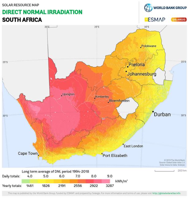
To determine the energy potential, we use the Direct Normal Irradiance (DNI) from the Global Solar Atlas. These three cities represent the high-potential interior, the moderate coastal-west, and the lower-potential coastal-east.
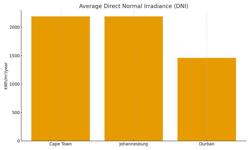
- Johannesburg (Max): DNI = 2191 kWh/m²/year
- Cape Town (Average): DNI = 2144 kWh/m²/year
- Durban (Min): DNI = 1461 kWh/m²/year
Step 2 |We convert the annual kWh values into a constant power density using the exercise's specific conversion factor: 1 kWh/m²/year = 0.11 W/m²
Power (W/m²) = (Energy (kWh/m²/year) × 1000 Wh/kWh) / (365 days × 24 h/day)
This reduces to multiplying by approximately 0.114155 (exact) but the dataset uses 0.11 as an operational conversion factor. Using 0.11 simplifies rounding and is consistent with the project dataset
Note: small differences in the final digit may arise from the use of 0 11 vs the exact conversion
Fig 1, Map of Direct Normal Irradiance (DNI) in South Africa | Figure 2: Average Direct Normal Irradiance values for South African cities
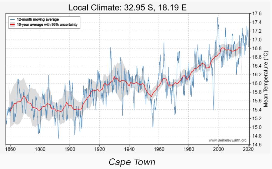
Step 4 | Research of the historical time series and projections of mean annual temperatures for the three selected cities.
The data in Fig. 3, 4, 5 highlight a significant divide in South Africa's solar resources, with inland/western cities (Johannesburg/Cape Town) possessing a much higher net radiation potential compared to the eastern coastal city of Durban.
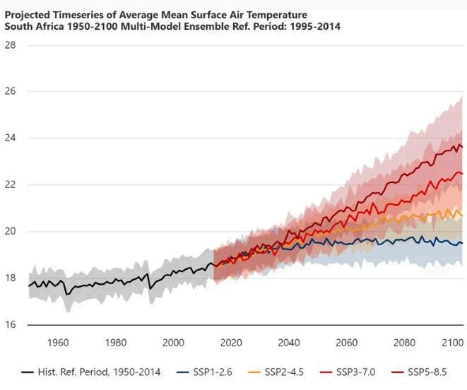
All three cities have experienced clear historical warming Looking forward, the country faces a high risk of severe mean temperature increase under high-emissions scenarios (SSP5-8.5), which could result in an increase of up to 8°C by 2100
1.3. Interpretation and Implications
Higher Rn corresponds to greater available energy at the surface, which generally increases land surface temperature (LST) and can result in higher urban heat loads. The difference between Cape Town/Johannesburg and Durban highlights the influence of local climatology (marine influence, cloud cover) on net radiation.
1.4. Recommendations and Uncertainty Analysis
Recommendations:
- Use Land Surface Temperature (LST) mapping to identify "Heat Islands" in Johannesburg. For Durban, focus on ventilation and humidity control, as lower Rn is often due to cloud cover and moisture.
- Uncertainty Note: The empirical formula used has an uncertainty of ±10%. Actual Rn can be lower in cities with high air pollution/smog which blocks incoming light. Uncertainty considerations:
- Conversion factor approximations: using 0.11 introduces a small systematic difference (±5% order).
- Empirical formula is regionally calibrated and may carry systematic bias; report an uncertainty band of approximately ±5–10% for diagnostic purposes.
2. EMISSIONS INVENTORY AND NDC LINKAGE
This section provides a detailed analysis of the key climate change metrics for South Africa and the city of Cape Town. The core objective is to collect and disaggregate data on CO2 emissions and interpret the NDC targets to construct an integrated understanding of the climate vulnerabilities and commitments of both the nation and its representative urban area.
Fig 3, 4, 5 Historical time series mean annual temperatures in Cape Town Johannesburg and Durban
Fig. 6. Projected mean annual temperature trends under different RCP scenarios
2.1. Data summary and Context
Key data points provided:
- The CO2 emissions by Country
- The CO2 emissions by City
- The Nationally Determined Contributions (NDCs) with a focus on the cities
- The Adaptation and Mitigation Strategies already set up
- The Adaptation and Mitigation Strategies you can add
2.2. Methodology for Disaggregation
A practical methodology to disaggregate municipal emissions:
a. Identify available local data: electricity consumption by sector (residential, commercial), transport activity (vehicle-km), industrial energy use, and waste processing quantities.
b Where local data exist, allocate emissions directly using activity data and emission factors.
c. Where local data are missing, apply sectoral proportions from national inventories adjusted by local indicators (e.g., population share, GDP share, industrial presence).
2.3. South Africa’s Emissions Profile
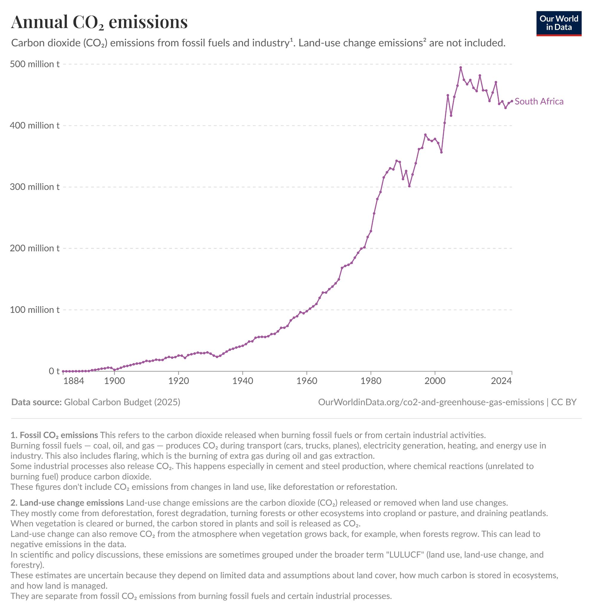
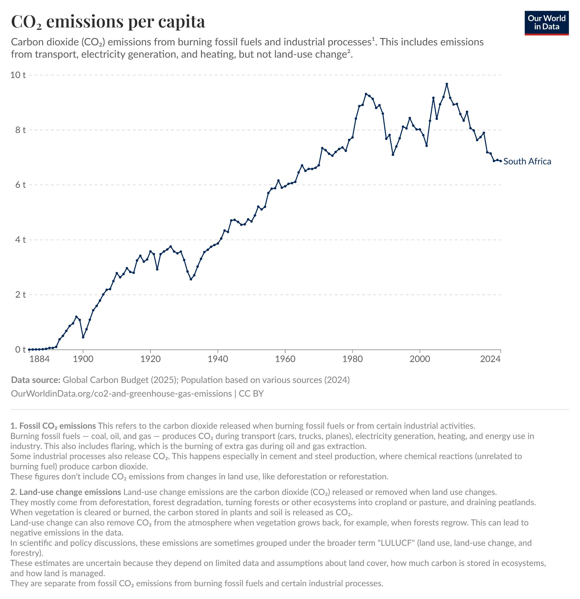
South Africa's Annual CO2 emissions from fossil fuels and industry have followed a dominant long term upward trajectory since 1884. Emissions began near zero and experienced initial gradual growth until the 1940s, after which they entered a period of exponential increase corresponding to intense industrialization. This sharp rise pushed emissions to a peak near 500 Mt around 2008/2009. In the most recent decade, the trend has shifted toward stabilization with a slight net decrease, with current emissions fluctuating around 430–440 Mt.
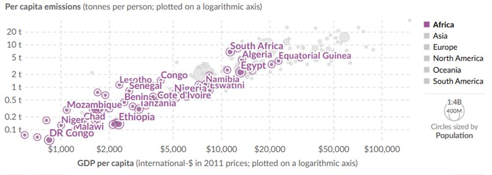
Globally, South Africa is typically ranked among the top 15–20 total CO2 emitters. However, due to its heavy reliance on coal for electricity generation, it ranks significantly higher per capita, often placing within the global top 10. Under the UNFCCC, South Africa is designated as a non-Annex I country.
Fig 7 Annual CO2 Emissions
Fig 8 CO2 Emissions per Capita
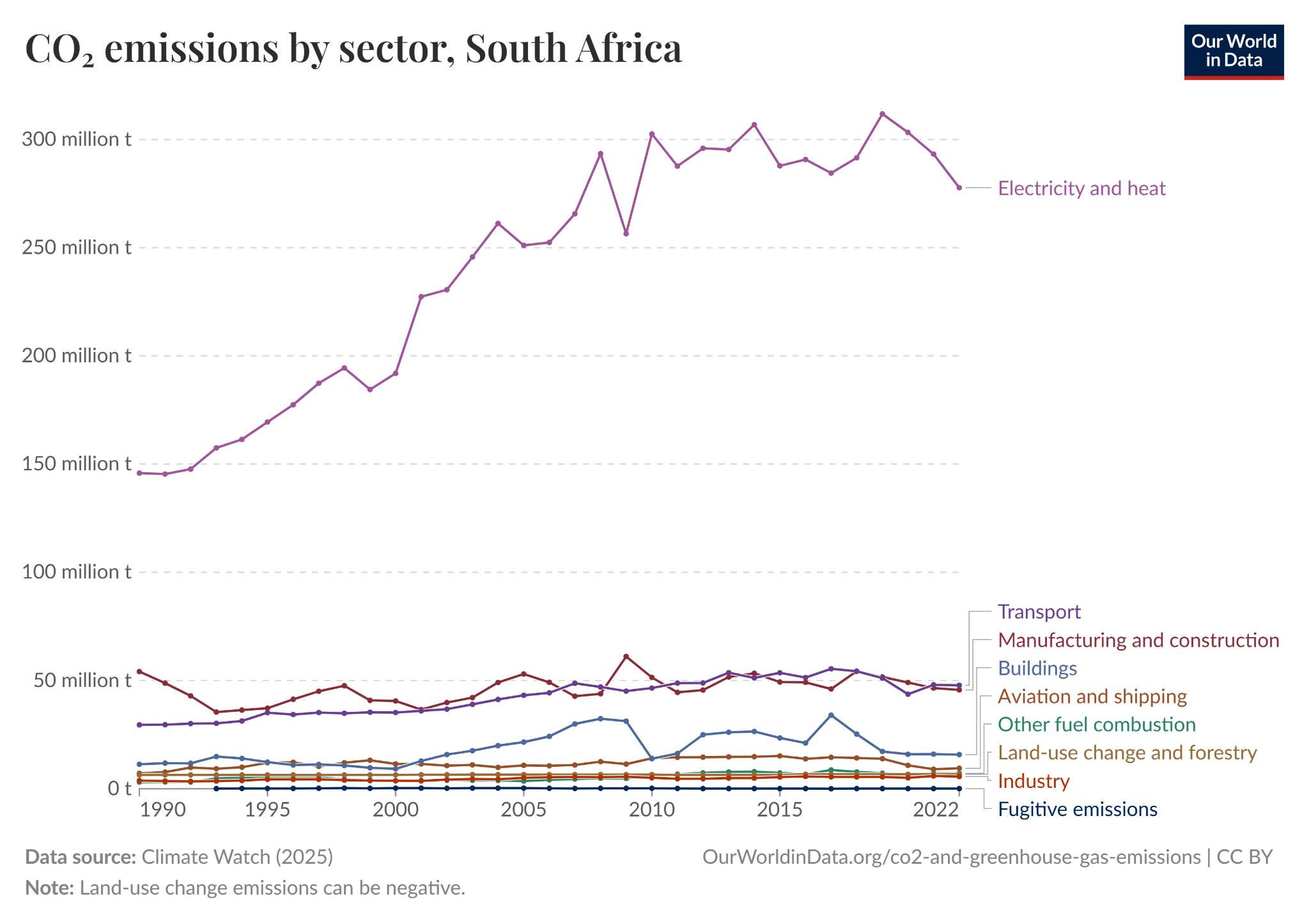
This severe emissions profile is driven by South Africa's energy sector, contributing approximately 70% = 280 MtCO₂ of the nation's total CO2 in 2022
Data from the International Energy Agency (IEA) shows that the residential sector accounts for 24.3% of total electricity final consumption in the country, around 68.04 MtCO2. When combined with the direct CO2 emissions from the buildings sector (10MtCO2), the total CO2 emissions for the Residential Sector reach approximately 78.04 MtCO2.
The Transport Sector is also a major source, contributing an estimated 50MtCO2, or approximately 12.5% of total national emissions.
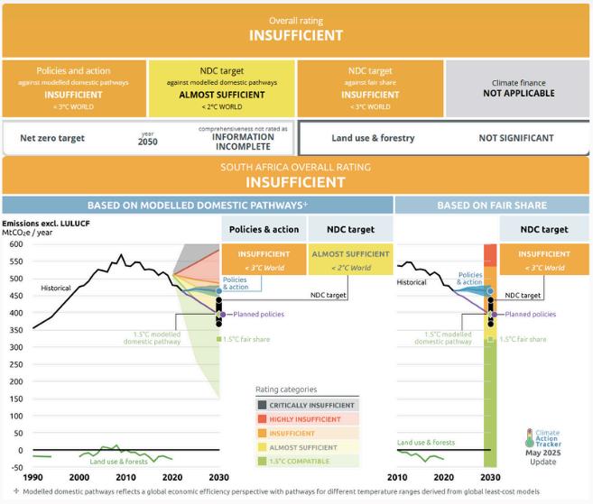
This "Insufficient" overall rating means South Africa's commitments and policies are not consistent with holding warming below 2℃, let alone the 1.5℃ limit of the Paris Agreement
The current Policies and action are rated "Insufficient", meaning South Africa is currently not on track to meet its own NDC target. While the NDC target is rated "Almost Sufficient" when judged against the domestic pathway, it drops to "Insufficient" when assessed against South Africa's fair share of global effort, indicating a significant ambition gap based on equity.
Based on the national emissions profile, the sector with the greatest impact on South Africa's CO2 emissions and climate action pathway is overwhelmingly the Electricity and Heat sector This sector is the primary source of the high emissions, driven by the country's heavy reliance on coal. Decarbonizing this sector is the main challenge and the biggest opportunity for South Africa to move its domestic modelled pathway closer to the 1.5℃ compatible range.
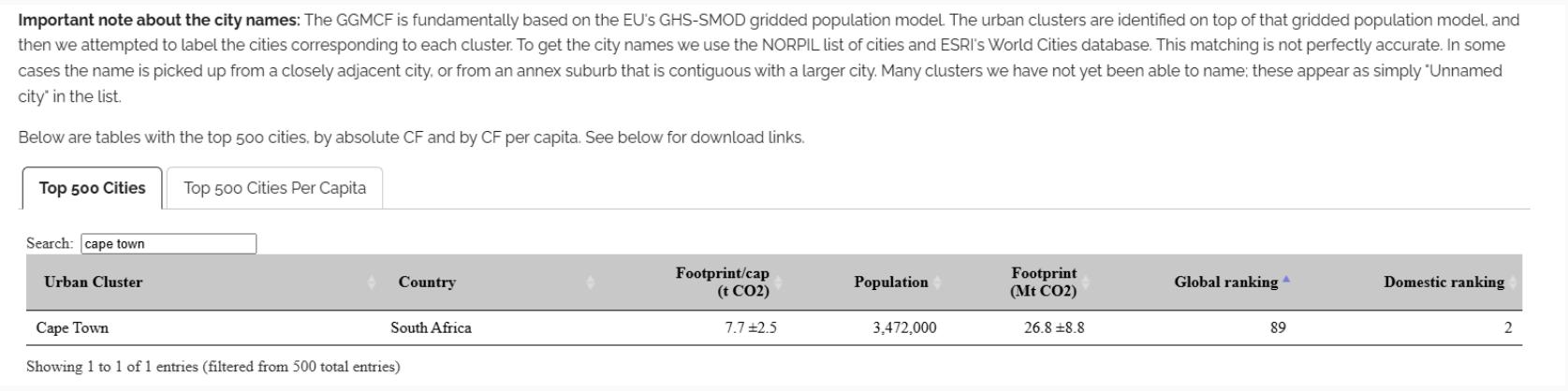
Cape Town's carbon footprint, when adopting the precautionary approach and selecting the higher available estimate, is approximately 26.8 MtCO2. This figure places the city as the 89th largest emitter globally and the second largest domestically within South Africa. This positioning underscores Cape Town's status as a significant urban contributor to national and global emissions, making it a critical focus area for the subsequent sectoral distribution and development of local mitigation and adaptation strategies.
Fig 9 CO2 Nation’s Emissions by Sector
Fig 10 Climate Action Tracker
2.4. Cape Town’s Emissions Profile
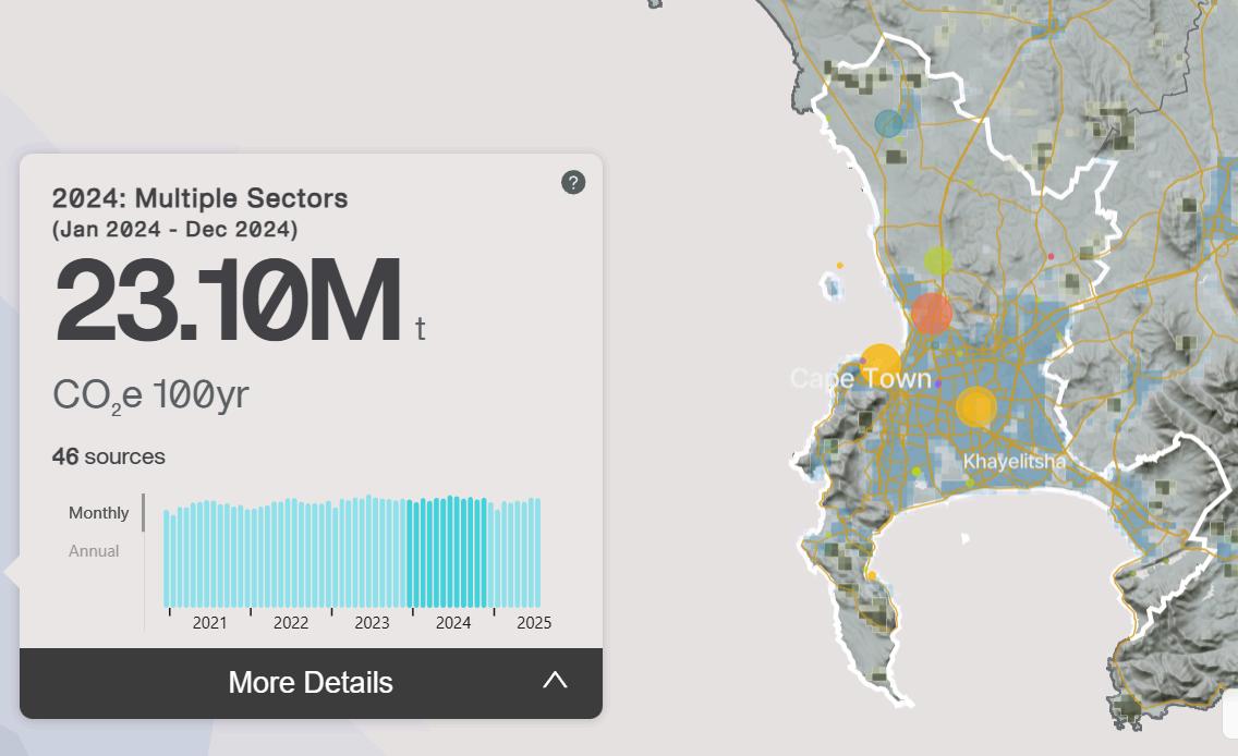
Fig. 11. Cape Town’s GGMCF Model
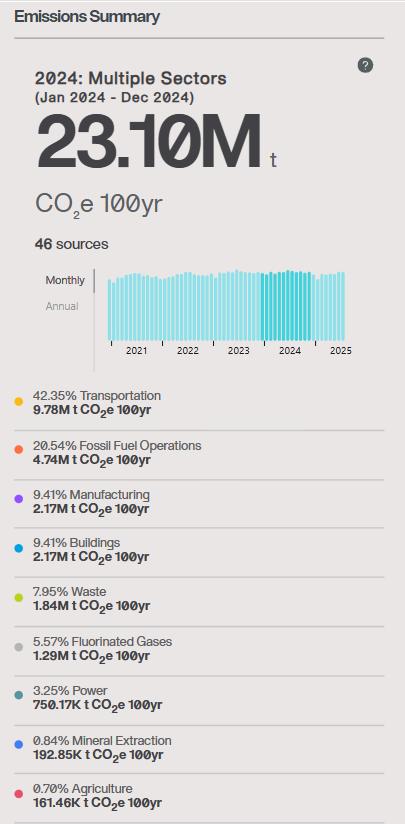
Cape Town's total CO2 equivalent emissions are 23.10 Mt, featuring an urban emissions profile that contrasts sharply with South Africa's national power-dominated average.
- The city's primary challenge is the Transportation sector, which is the largest source, responsible for 42.35% of the city’s footprint.
- The next significant contributor is Fossil Fuel Operations with 20.54%.
- The Buildings sector and Manufacturing are tied as the third-largest sources, each contributing 9 41%
- Critically, direct emissions from the Power sector within the city limits are extremely low, accounting for only 3.25%, indicating that city-level mitigation efforts must focus strategically on mobility and fuel use, rather than local power generation.
2.5. Nationally Determined Contributions
South Africa’s NDC highlights energy efficiency in buildings as a key mitigation measure. It plans to strengthen building codes, retrofit existing structures, and promote low-carbon design. Urban areas are explicitly identified as priority zones for adaptation and resilience, focusing on water, energy, waste, and disaster management. The NDC promotes urban greening, reforestation, and ecosystem restoration as part of climate adaptation.
South Africa’s Second NDC (2025) commits the country to:
I. Mitigation Strategies
A. PPD Trajectory: Committing to a Peak, Plateau, and Decline (PPD) trajectory for national greenhouse gas emissions, establishing fixed-level target ranges for 2025 and 2030.
B. Energy Transformation: Implementing a complete transformation of the future energy mix to transition away from inefficient, aging coal-fired power plants.
C. Decarbonization Focus: Driving substantial investment in renewable energy ( wind and solar) and rolling out programs to increase efficiency and reduce emissions intensity across various economic sectors.
II. Adaptation Strategies
A. NAP Development: Developing and implementing a National Adaptation Plan (NAP), which is integrated into all relevant sectoral plans and serves as the official adaptation communication.
B. Vulnerability Assessment: The NAP is informed by a comprehensive assessment of sectoral, cross-sectoral, and geographical vulnerabilities to climate change impacts.
C Integrated Planning: Integrating specific adaptation planning at sub-national and local levels into development frameworks and land-use schemes.
D. System Development: Building institutional capacity, and developing an effective early warning vulnerability and adaptation monitoring system to track progress and impacts.
Fig. 12. Cape Town’s CO2 Annual Emissions
2.6. Translating NDCs to Local Targets
The national climate framework requires a specific localization of effort to effectively address Cape Town's unique challenges.
For mitigation, the national priority of transforming the coal-dominated energy system translates locally into:
● Targeted Transport Decarbonization. Aggressively investing in public transit, Non-Motorized Transport (NMT), and EV infrastructure to tackle the city’s single largest emission source (42.45%)
● Local Clean Energy Procurement. Seeking clean energy from Independent Power Producers (IPPs) and promoting rooftop solar PV to address the CO2 emissions embedded in the national grid used by buildings and industry.
● Green Building Standards. Enforcing stricter building codes and implementing retrofitting programs to manage the Buildings sector emissions (9.41%).
For adaptation, the NAP's focus on institutionalizing resilience and water security translates into:
● Water Resilience Implementing integrated resource management, desalination, and water recycling/reuse to safeguard against extreme drought, aligning with the NAP's priority on the vulnerable water sector.
● Urban Heat Management. Expanding Nature Based Solutions (NBS) like urban green spaces to mitigate the Urban Heat Island effect and improve air quality in human settlements.
● Infrastructure Protection. Enacting strict land-use planning and restoring natural coastal buffers to protect against sea-level rise and storm surges, as mandated by the national disaster management and settlements priorities.
2.7. Proposed Local Action Plan
➔ Main Goal (by 2030): Reduce the city’s CO₂ emissions by 30% compared to current levels, while increasing resilience to heatwaves, droughts, and floods.
➔ Mitigation Strategies
- Urban Solar Expansion: Install solar panels on public and private buildings to supply 25% of the city’s electricity from renewables by 2030.
- Clean Transport: Electrify public buses, promote cycling, and restrict petrol vehicles in the city center.
- Energy-Efficient Buildings: Enforce Green Building Codes and retrofit old structures to improve efficiency.
- Smart Waste Management: Boost recycling to 60% and develop waste-to-energy plants.
- Urban Greening: Expand green areas and urban forests for carbon capture.
➔ Adaptation Strategies
- Climate Resilient Infrastructure: Upgrade drainage, water, and sanitation systems to handle floods and droughts.
- Water Sustainability: Promote greywater use, rainwater harvesting, and water-saving behavior.
- Cool City Initiative: Use reflective materials and green roofs to lower urban heat islands.
- Climate Education: Run awareness campaigns for citizens on sustainable living.
- Social Resilience: Create green jobs and develop affordable, climate-friendly housing.
2.8. PV Potential Estimation (link to Exercise 1)
Use Snet (DNI-derived W/m²) to estimate rooftop PV potential.
Steps:
a. Estimate usable rooftop area (m²) from cadastral or land-use data.
b Multiply by specific yield (kWp/m²) to get installed capacity potential
c. Multiply capacity by specific annual production (kWh/kWp) estimated from DNI to get annual energy.
d. Convert energy to emissions avoided using a grid emission factor (kgCO₂/kWh).
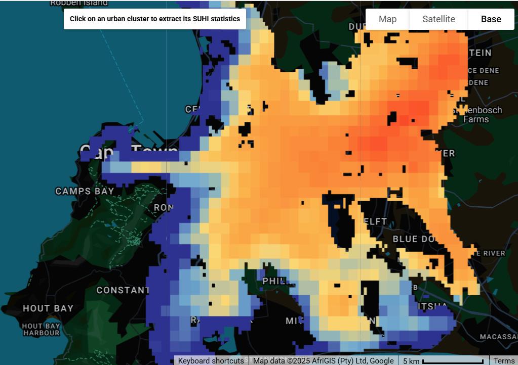
3. SUHI AND TREE COVER ANALYSIS
This exercise examines the Urban Heat Island (UHI) phenomenon in Cape Town with a focus on Surface Urban Heat Island (SUHI) intensity, tree cover availability per capita, and projected temperature changes toward 2050 The objective of the analysis is to evaluate current thermal conditions and identify spatially informed climate adaptation opportunities.
3.1. SUHI Definitions, Data Sources and Interpretations
The Urban Heat Island (UHI) effect describes the temperature difference between urbanized areas and their surrounding rural context In this study, the Surface Urban Heat Island (SUHI) Intensity is used and defined as:
SUHI =
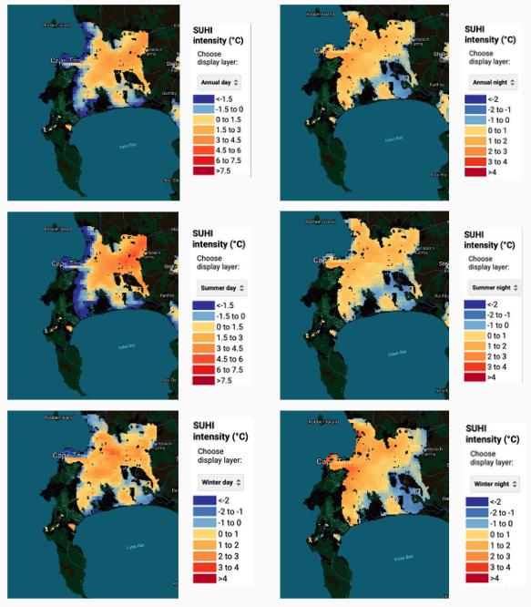
SUHI values were obtained from the global surface UHI explorer developed by the Yale Center for Earth Observation. For this exercise, the Cape Town urban cluster was selected, and the summer daytime SUHI value for 2020 was extracted.
● Observed Summer Daytime SUHI: 0.83 °C
● Reference threshold: 1.5 °C (values above this level indicate a likely UHI effect)
Based on this dataset, Cape Town’s average summer daytime SUHI remains below the commonly used threshold. This suggests that, at a city wide scale, a pronounced urban heat island effect is not evident.
However, this average value does not fully capture local thermal conditions. Several local and regional studies report daytime surface temperature differences of up to 3–5 °C in inland and densely built districts such as Bellville and Maitland. These localized hotspots indicate that while the overall SUHI signal is weak to moderate, spatial variability across neighborhoods is significant.
Cape Town’s coastal location, prevailing sea breezes, and relatively high levels of urban vegetation contribute to moderating surface temperatures, particularly in areas closer to the coastline. At the same time, inland urbanized zones with limited vegetation experience higher thermal
stress, highlighting the importance of localized analysis rather than reliance on city-wide averages alone.
3.2. Tree Cover per Capita
This section evaluates the existing green infrastructure in Cape Town by measuring the available tree cover area against the population, using the World Health Organization (WHO) benchmark of 15 m2 per person as a minimum target. The City of Cape Town currently possesses 32.2 kha of tree cover with greater than 30% canopy density.
According to available municipal data, the City of Cape Town contains approximately 32 2 kha of tree cover with canopy density exceeding 30%. Using a metropolitan population of 3,472,000 inhabitants, tree cover per capita was calculated as follows:
Tree cover per capita = Tree cover area (m²) / Population
● Tree cover area: 32.2 kha = 322,000,000 m²
● Population: 3,472,000
Tree cover per capita ≈ 92.7 m²/person
This value significantly exceeds the WHO (World Health Organization) minimum recommendation, indicating that Cape Town possesses a strong overall green asset that supports passive cooling and urban resilience.
Nevertheless, this result requires careful interpretation A large share of the total tree cover is concentrated in natural reserves, mountainous terrain, and peripheral green areas, rather than within densely populated urban neighborhoods. As a result, many residential areas particularly within The Cape Town experience low local canopy coverage, despite the high city average. These areas are more exposed to heat stress and benefit less from the cooling potential of urban vegetation.
3.3. Temperature Projections
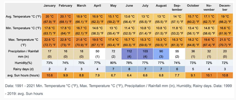
Cape Town’s Mediterranean climate, characterized by warm dry summers and mild wet winters, makes the city particularly sensitive to gradual warming and increased drought risk.
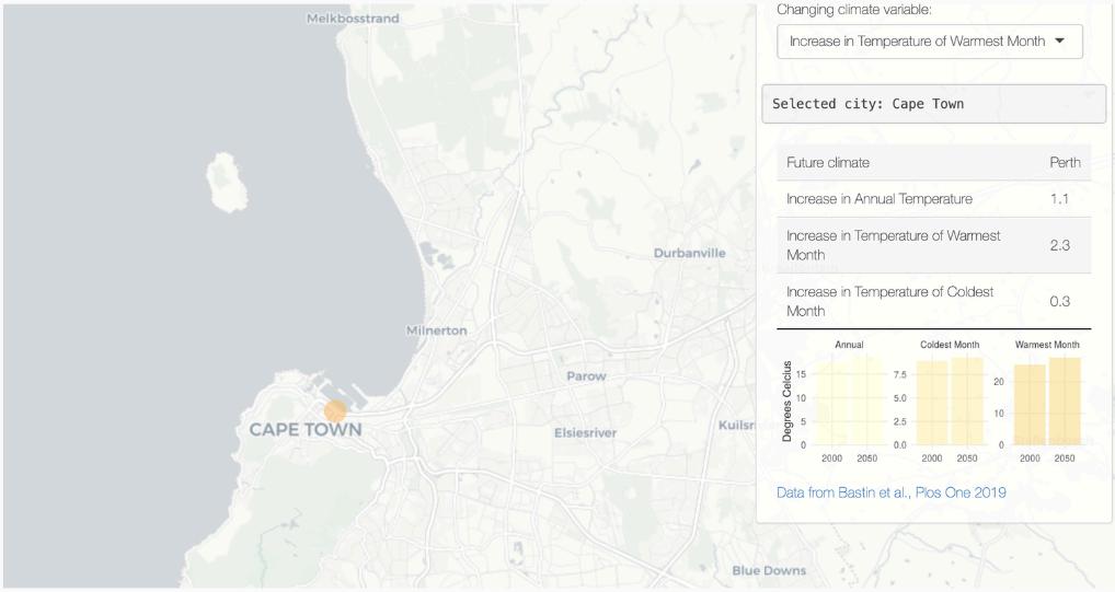
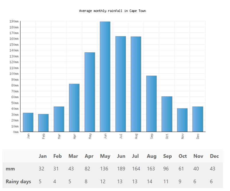
At present, february is the warmest month with an average temperature of 20.1 °C, while July is the coldest at 13.0 °C, resulting in an annual mean temperature of 16.4 °C (Fig. 13).
Climate projections indicate a consistent warming trend aligned with global models for coastal Mediterranean type regions.
Fig 13 Climate data for Cape Town
By 2050, the annual mean temperature is projected to increase by approximately 1.1 °C. The warmest month is expected to warm by up to 2.3 °C, while winter temperatures show a smaller increase of around 0.3 °C. Under these conditions, Cape Town’s future climate is anticipated to resemble that of present day Perth, Australia.
In parallel, summer daytime SUHI intensity is projected to rise from approximately 0.85 °C to 1.3 °C by 2050 (Fig 14) Although still below the 1 5 °C threshold, this increase reflects enhanced surface heating associated with continued urban expansion, land use change and reduced vegetative cover in some areas.
3.4. Spatial Analyses and Recommendations
To support targeted climate adaptation strategies, a spatially explicit workflow is recommended:
● Derive canopy cover maps using Sentinel 2 imagery (10–20 m resolution) or higher resolution data where available
● Compute land surface temperature (LST) from Landsat or ECOSTRESS datasets for comparable clear sky dates to generate SUHI maps.
● Overlay SUHI intensity, canopy cover, population density, and socio economic vulnerability indicators to create a composite priority index.
● Identify intervention locations such as streetscapes, parks, and rooftops, and estimate potential cooling benefits.
Previous studies indicate that concentrated urban greening interventions, including street trees and parks, can produce local air temperature reductions of approximately 0.5–1.5 °C, depending on design and density Green roofs and walls can further complement street level measures by reducing surface temperatures and lowering building energy demand.
This analysis is constrained by the spatial resolution of global SUHI datasets and the aggregation of tree cover statistics at the metropolitan scale. As a result, neighborhood-level heat exposure particularly in socially and economically vulnerable districts may be underestimated. More detailed local measurements would be required to fully capture micro-scale thermal variations.
4. INTEGRATED FLOOD AND HEATWAVE RISK (DUAL HAZARD)
This section describes the integrated methodology adopted to quantify the simultaneous exposure to pluvial flooding and heatwave events within the study area. The approach consists of a sequential evaluation of hazard, exposure and vulnerability for each hazard type, followed by the construction of a composite multi-hazard risk index
Fig. 14. Data from Future Cities showing Cape Town’s future projections
4.1. Flood Peak Estimation (Rational
Method)
Methodological
Framework
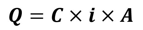
Flood peak discharge was estimated using the Rational Method: where:
● is the peak discharge (m³/s),
● is the runoff coefficient,
● is the rainfall intensity (mm/h)
● is the drainage area (km²).
The study area covers 30 ha = 0.30 km².
A runoff coefficient of C=0.6 was adopted, consistent with mixed urban fabrics.
The selected critical rainfall duration is t=30min, which is consistent with the time of concentration of catchments of comparable extent.
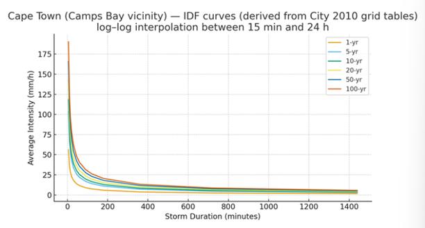
IDF Curves: Data Collection and Application
Rainfall intensities for several return periods were derived from the local IDF curves provided in the course materials. These values were directly used to compute the design discharges using the Rational Method.
Design Discharge Calculation
The table below reports the adopted rainfall intensities and the resulting discharges:
The mm/h → m³/s conversion used the standard factor 1000/3600.
Drainage System Capacity
Project documentation specifies that drainage capacity should be defined as the 10-year peak discharge increased by 20%, to account for potential rainfall intensification and long-term efficiency losses:
Identification of the Critical Return Period T*
Comparing design discharges with the drainage capacity:
Q (20) = 2.33 < 2.40 m³/s
Q (50) = 2 76 ≥ 2 40 m³/s
Thus, the first return period for which discharge exceeds system capacity is:
The associated annual exceedance probability is:
Earlier drafts reported T*=5years; this discrepancy originates from the use of an undocumented drainage capacity (~1.6 m³/s). In the absence of supporting evidence, the value following the stated specification (Q 10×1.20) has been retained.
Flood Hazard Classification
A five-class hazard scale based on annual exceedance probability was adopted:
P ≤ 0.01 → Hazard = 1
0.01< P ≤0.05 → Hazard = 2
0.05 < P ≤ 0.10 → Hazard = 3
0.10 < P≤ 0.20 → Hazard = 4
P > 0.20 → Hazard = 5
With P = 0.02, the flood hazard is:
4.2. Exposure and Vulnerability to Flooding
Exposure
Exposure was quantified based on population density (GHSL or equivalent), economic activities, and the presence of critical infrastructure within the AOI.
The coastal portion of the area shows high density and elevated economic value; therefore:
Vulnerability
Vulnerability was assessed considering general building characteristics, accessibility, ground-floor exposure, and functional aspects. In the absence of clear fragility indicators, aggregated vulnerability was classified as:
4.3. Flood Risk Assessment
Risk was computed as:
Normalizing over the theoretical maximum (125):
Therefore, Flood risk is low to moderate, although local hotspots persist due to the high exposure.
4.4. Heatwave Hazard, Exposure and Vulnerability
Operational Definition
Heatwaves were defined as periods with at least one day (or multiple consecutive days) where maximum temperature exceeds either:
- the 95th percentile of historical maxima, or
- a fixed threshold of 35°C, adopted here due to the limited temporal extent of the dataset
Because the available dataset covers only June–July 2010 (winter season) and does not include long-term climatological records, the 35°C threshold was used.
Dataset Description
The dataset extracted from Google Earth Engine (GEE) contains:
- daily Land Surface Temperature (LST) values (day and night)
- geolocation and date attributes
- for the period 1 January – 1 February 2023
- approximately 30 days of data
LST Day C ranges between 24.43°C and 36.27°C .
Heat Hazard Identification
Each day was evaluated to check whether LST Day C exceeded the 35°C threshold
● Total days analysed: ~30
● Days above 35°C: 5
2023-01-01:36.25 °C
2023-01-02:36.27 °C
2023-01-07:35.59 °C
2023-01-08:35.17 °C
2023-01-17:35.13 °C
● Hot-day percentage: 5/30×100% ~ 16.7%
Heat Hazard Classification
A five-class scale was applied:
Since no hot days were recorded:
Heat Exposure (E heat)
Exposure to heatwaves was evaluated considering:
- population density
- concentration of economic and service functions
- critical infrastructure distribution
Despite the low seasonal hazard, the structural exposure of the urban area remains high:
4.5. Urban Green Factor (UGF) Assessment for Heatwave Mitigation
To complement the dual-hazard analysis, the Urban Green Factor (UGF) was computed to quantify the spatial distribution, quality, and contribution of urban green surfaces to local cooling capacity.
This indicator supports the identification of areas where low vegetation cover exacerbates heatwave vulnerability and where nature-based solutions would be most effective.
Definition of Input Data
In the context of Google Earth Engine (GEE), input data refers to the datasets used as the basis for spatial analysis.
For the UGF computation, three categories of input data were employed:
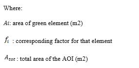
Area of Interest (AOI)
The administrative boundary of the Cape Town urban area was imported as a Feature Collection. This polygon defines the spatial limits of the analysis and is used to clip all subsequent datasets.
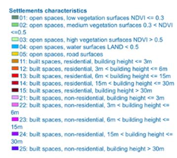
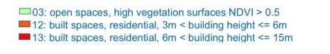
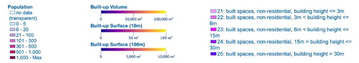
Satellite-Based Surface Information
High-resolution Earth observation data were used to identify vegetation, permeable surfaces, and impervious urban fabrics. Specifically:
- Sentinel-2 MSI imagery (COPERNICUS/S2) was filtered by date, cloud coverage, and spatial bounds to derive vegetation indices (e.g., NDVI) and discriminate green areas.
- Copernicus Global Land Cover (100 m) was used to classify surface types (grass, trees, bare soil, impervious cover) and to assign weighted factors within the UGF formula.
Surface Classification Layers
Building on the selected imagery, surfaces were categorized into green, permeable, and impermeable classes through spectral thresholds and existing land-cover labels. These classes serve as the quantitative base for the UGF calculation. Thus, the input data consists of the combination of AOI + selected satellite imagery + land-cover datasets, which collectively provide the raw information from which green area proportions were extracted
Methodology in Google Earth Engine
The UGF was calculated following a fully automated workflow in GEE:
● AOI Delimitation
The boundary of the Cape Town metropolitan area was uploaded and used to clip all datasets.
● Data Import
Sentinel-2 level-2A imagery and Copernicus Land Cover products were retrieved as input datasets.
Filters were applied for:
- date range (year of analysis),
- cloud cover (e.g., < 20%),
- intersection with the AOI.
● Surface Classification
Using spectral indices (NDVI) and land-cover classes, surfaces were grouped into:
- vegetated/green areas (trees, grass, urban parks),
- permeable surfaces (bare soil, green roofs, permeable pavements),
- impervious areas (roads, buildings, asphalt).
Weight Assignment
Each surface type was associated with a weight (fi), reflecting its cooling potential (e.g., trees > grass > permeable soil > impermeable cover).
UGF Calculation
The Urban Green Factor was computed as:
GEE automated the pixel-based computation and produced both the mean UGF value and its spatial distribution.
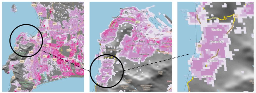
Results and Interpretation
The analysis yielded:
- Mean UGF = 0.43
- UGF percentage = 42.9% (weighted green surfaces)
These values indicate a moderate level of urban greening. Coastal districts such as Camps Bay show a relatively balanced mix of vegetation and built-up areas, contributing to local cooling. However, the overall UGF is below the commonly suggested threshold of 0 6–0 7, typically recommended for heat-resilient urban environments.
Areas with lower UGF coincide with densely built districts, which are more susceptible to surface urban heat island (SUHI) amplification, reinforcing their classification as heatwave “hotspots”
Heat Vulnerability (Vheat)
Vulnerability to heat was derived from the Urban Green Factor (UGF).
The GEE-based analysis yielded:
Using the vulnerability scale:
UGF ≥ 0.6 → Vulnerability = 1
0 4 ≤ UGF < 0 6 → Vulnerability = 3
UGF < 0.4 → Vulnerability = 5
Thus:
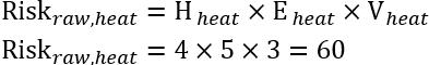
4.6. Heat Risk Assessment
Heat risk is computed using the multiplicative approach:
Normalizing over the maximum value (125):
Heatwave risk during the analysed period is therefore Moderate–high.
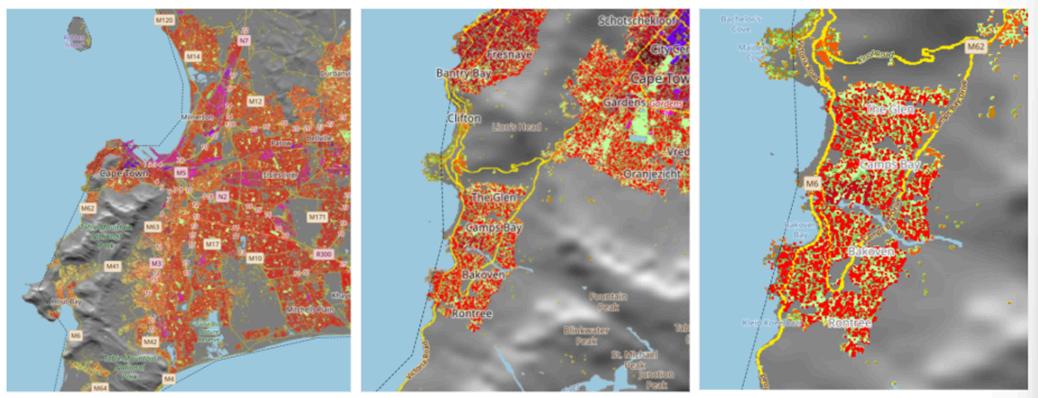
4.7. Integrated Risk Mapping (Dual Hazard)
A composite multi-hazard index was computed as:
This equal-weight formulation enables balanced consideration of the two hazard types
Risk maps highlight:
- areas with high combined hazard,
- zones where low UGF, high exposure and local drainage limitations coincide, - districts where nature-based solutions (green corridors, increased tree canopy, permeable surfaces, bioswales) can deliver co-benefits against both heat and pluvial flooding.
The integrated analysis shows that:
- Flood risk is moderate, primarily driven by high exposure rather than hazard levels.
- Heat risk is low for the analysed winter period, but structural exposure and limited green coverage suggest potential vulnerability during summer
- The UGF value (0.43) highlights the need for targeted green-infrastructure interventions to reduce thermal vulnerability.
- The dual-hazard framework effectively reveals areas where interventions provide simultaneous resilience benefits, supporting robust and adaptive urban planning strategies.
5. URBAN GREENING FACTOR ANALYSIS
The Urban Greening Factor (UGF) is an index that quantifies the contribution of different surface types to urban green infrastructure, weighted by their effectiveness for cooling, infiltration, or biodiversity. The core purpose in this exercise was to diagnose the district’s current environmental performance, quantifying its capacity to mitigate the Urban Heat Island (UHI) effect and manage stormwater runoff.
5.1. Site Selection and Definition
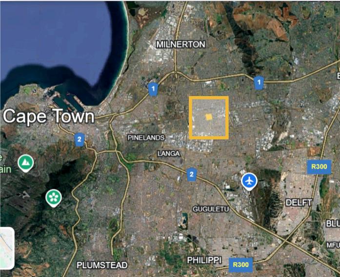
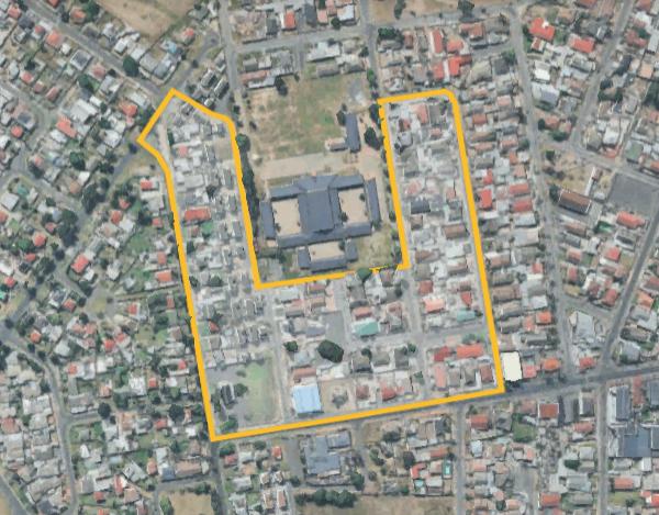
The site selection was consistent with the findings from previous exercises, which identified the city's areas exhibiting the highest Surface Urban Heat Island (SUHI) intensity.
The chosen area was the suburbs of Ruyterwacht and Riverton. This residential/mixed use area, characterized by dense housing, highly impervious surfaces, and limited vegetation, was identified as a critical zone for climate vulnerability analysis due to its elevated SUHI values. The selected area has 60,174.02 m² and it was chosen by using Google Earth Engine tool to confirm the area's thermal characteristics.
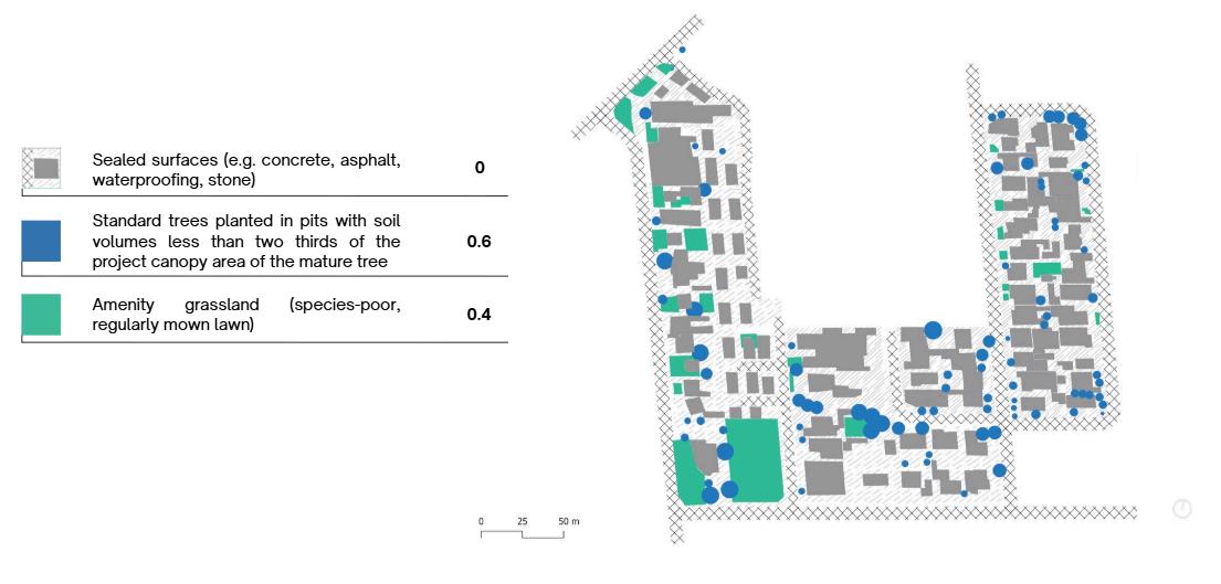
5.2. Surface Quality Mapping and UGF Score Assignment
Using satellite imagery and a standardized UGF scoring table adapted from the London Green Factor Guide, every square meter of the site was mapped and categorized. Surface cover types, such as sealed concrete, amenity grassland, and areas with planted trees, were assigned a UGF Factor based on their ecological function
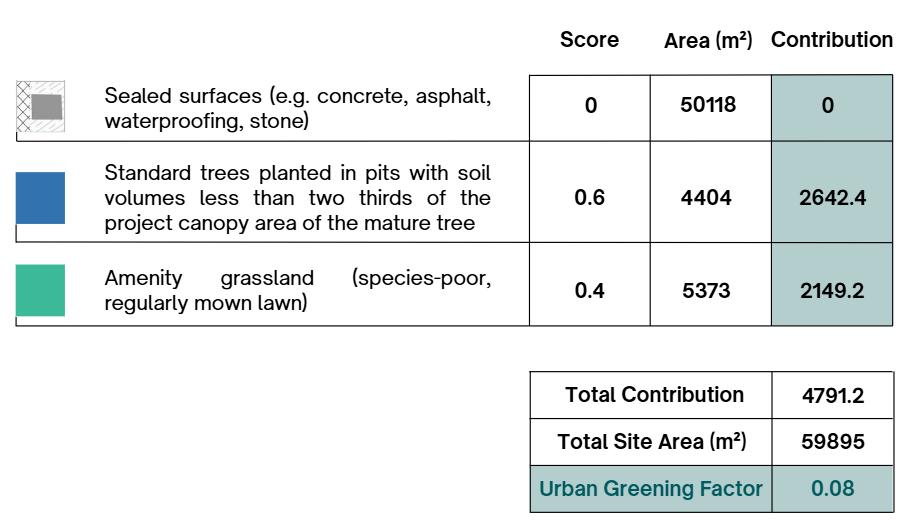
5.3. UGF Calculation
The Urban Greening Factor was calculated using the formula:
UGF = ∑ (Surface Type Area x Assigned Score) / Total Site Area
The area of each categorized surface was measured in square meters, multiplied by its assigned factor, and summed to determine the Total Contribution. This total contribution was then divided by the Total Site Area of 59,895 m²
The final calculated UGF score for the Ruyterwacht and Riverton area is 0.08.
5.4. Performance Assessment
The calculated score of 0.08 is significantly below the minimum required benchmark of 0.4 This confirms that the current land cover offers a negligible contribution to mitigating UHI and managing stormwater runoff, consistent with the initial selection of the area due to its high Surface UHI (SUHI) intensity.
5.5. New Target and Proposed Strategies
● Future UGF Target: 0.45
This target requires converting nearly half the surface area into medium to high factor green infrastructure, a contribution increase from 4,791.2 to ≈ 26,953. Achieving this confirms a robust strategy for UHI and stormwater management in the Ruyterwacht and Riverton district
The proposed Urban Adaptation Strategies are:
➔ Intensive Green Roofs. Target all suitable flat roof spaces for intensive green roofs (factor = 0.8) to provide deep-rooting native vegetation for maximum evaporative cooling and shading.
➔ Linear Parks and Street Trees. Convert sealed road verges and non essential parking areas into linear green spaces with standard trees planted in connected pits (factor = 0.8) to create shaded street canyons, enhancing pedestrian comfort
➔ Rain Gardens and Swales. Introduce rain gardens and vegetated sustainable drainage systems (factor = 0.7) in strategic locations to capture and infiltrate stormwater runoff.
➔ Permeable Paving. Replace existing sealed parking lots and pedestrian walkways with permeable paving (factor = 0.1) to allow rainwater infiltration.
➔ Cool Pavement Apply cool pavement coatings to necessary roads to increase their albedo and reduce heat absorption.
CLIMATE RESILIENCE ANALYSIS FOR CAPE TOWN - ACADEMIC REPORT #2
INTRODUCTION AND OBJECTIVES
This study addresses South Africa's dual climate challenge by integrating national level emission forecasting with local urban adaptation strategies centered on ecological justice. By analyzing demographic trends and projected economic growth, our study establishes a climatic profile for the country, correlating CO2 emissions with GDP through near future projections. Simultaneously, the research shifts to the neighborhood scale in Cape Town to address hydraulic vulnerability. This comprehensive approach ensures that climate resilience is not only technically sound but also environmentally fair. The primary objective is to link national climate forecasting with local resilience planning by assessing the data gathered alongside identifying spatial and thermal injustices. To achieve this, the study aims to map specific social vulnerabilities to ensure that proposed Nature Based Solutions are equitable and inclusive. Furthermore, the research focuses on the technical design and sizing of Sustainable Drainage Systems (SUDS), such as bioretention areas and rain gardens, to manage excess stormwater volume and mitigate flood risk. Finally, the study seeks to evaluate these interventions by recalculating the Urban Greening Factor and providing a comprehensive design strategy to demonstrate improved local ecological quality.
6. POPULATION GROWTH AND CO2 EMISSIONS
This section examines the demographic and economic evolution of South Africa and evaluates how these dynamics will influence national CO2 emissions over the coming decades. The goal is to integrate population trends, GDP projections, and emission estimates into a coherent assessment of the country’s expected climate profile, expanding the analytical framework developed.
6.1. Demographic Projections
Methods and Data Assumptions
This analysis utilizes reliable international datasets and standard engineering assumptions. Demographic data (population, birth, and death rates) are sourced from the UN World Population Prospects (WPP 2024). Economic data (GDP and GDPpc in PPP) are drawn from the IMF Data Mapper and the World Economic League Table 2024. CO2 emissions are correlated with GDP using a validated empirical model. The central assumption in the CO2 projection is that no radical decarbonization policies are implemented, allowing economic growth to continue driving emissions
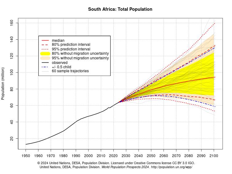
● Current Population
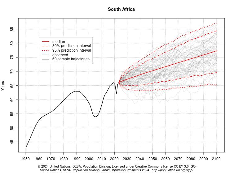
South Africa's population is estimated at approximately 64 million. The median projection displayed in the graphic shows the population will grow to approximately 74 million by the year 2038, representing a total increase of about 10 million people. The population is projected to continue growing rapidly toward the end of the century, nearing 90 million by 2070, but the prediction interval shows a wide range, indicating significant uncertainty, particularly regarding migration impacts. [1]
Fig. 1. South Africa’s Total Population and Projections
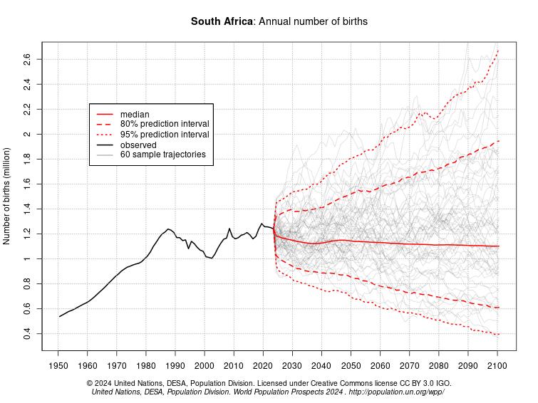
● Birth Rates
Despite the falling rate, the total number of births is currently around 1.2 million and is projected to slightly decrease to approximately 1.15 million by 2038 . This shows that the population increase is driven more by the current population structure than by a significant rise in the number of annual births [1]
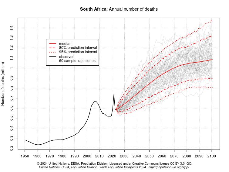
● Death Rates
The mortality data shows a notable spike in recent history and a clear rising trend for the future, likely reflecting population aging and health factors. The total number of annual deaths is currently around 0.6 million. The median projection shows a clear rise, with annual deaths expected to reach approximately 0.8 million by 2038. The current life expectancy encapsulating both genders is around 66 years old. [1]
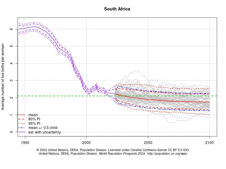
South Africa’s demographic data aligns with the transition from the Intermediate to Late Stage of the Demographic Transition Model (DTM), a phase characterized by a persistent and significant gap between the Crude Birth Rate (CBR) and the Crude Death Rate (CDR). The Crude Death Rate has stabilized at a low level due to public health advancements, however, the Crude Birth Rate, while declining from pre-transitional highs, remains sufficiently elevated to generate substantial population inertia.
Fig. 2. South Africa’s Annual Number of Births
Fig. 3. South Africa’s Fertility Rate
Fig. 4. South Africa’s Annual Number of Deaths
Fig. 5. South Africa’s Life Expectancy
6.2. Gross Domestic Product
Methods and Data Assumption
We're using the Purchasing Power Parity (PPP) methodology, measured by international dollars, to ensure results are compatible over time and across global economies.
The current economic baseline for this exercise is based on the International Monetary Fund (IMF) Data Mapper. The projection for total GDP growth is derived from the growth factor provided by the World Economic League Table of 2023.
● Current GDP (PPP)
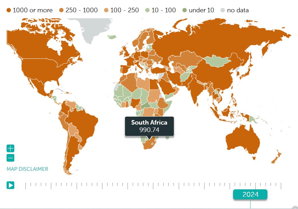
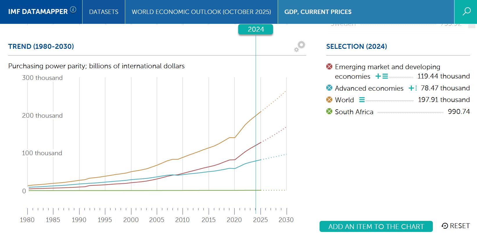
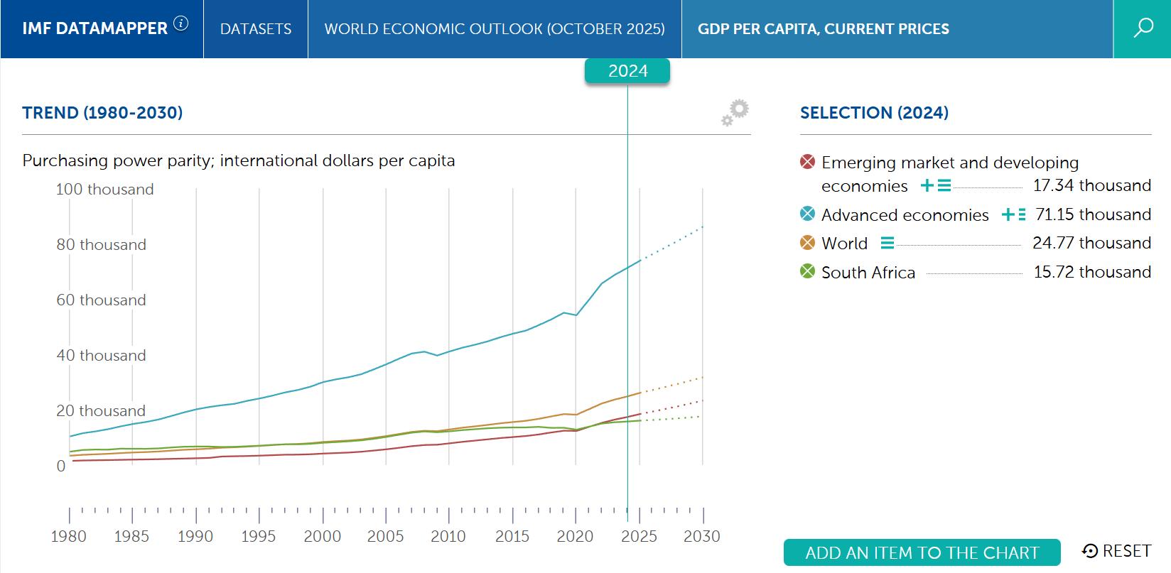
The International Monetary Fund's (IMF) Data Mapper as the economic baseline establishes that South Africa's Total Gross Domestic Product (GDP) in PPP terms for 2024 was around 990.74 billion USD. [2]
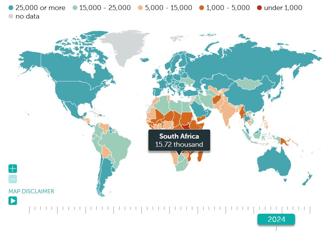
While the GDP per capita (PPP) for the same year was around 15.72 thousand USD. [2]
● Future GDP growth
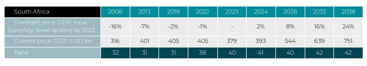
Future total GDP growth is based on the World Economic League Table projection, which anticipates a 22% increase in Constant Price GDP (local currency) between 2024 and 2038.
Fig. 6. South Africa’s GDP, Current prices. Purchasing power parity; international dollars per capita.
Fig. 7. South Africa’s GDP per capita, current prices Purchasing power parity; international dollars per capita.
Fig. 8. World Economic League Table 2024
Applying this growth factor of 1.22 to the 2024 Total GDP (PPP) grants a projected total GDP of 1,208.70 billion USD for 2038. [3]
● Future GDP per capita
This represents the expected output of the economy, adjusted for price changes For this calculation we know that the projected population for the target year 2038, based on the median estimate from the UN World Population Prospects, is around 74 million.
The projected GDPpc,2038 is calculated by dividing the projected Total GDP (1,1208.70 billion USD) by the projected population (74 million). This results in a GDPpc,2038 of 16,333 USD.
6.3. CO₂ Emission Estimates
To estimate future emissions, an empirical relationship linking GDP per capita and CO2 emissions per capita is applied. This correlation is widely used to describe how economic growth typically drives higher emission intensity in developing or fossil-fuel-reliant economies.
➔ Current Emissions (2024)
With a GDP per capita of 15,720 USD:
➔ Total National Emissions:
This aligns with the most recent national inventories, reflecting South Africa’s dependence on coal-based electricity generation.
➔ Projected Emissions for 2037
With an estimated GDP per capita of ~16,300 USD:
➔ Total Emissions:
South Africa could experience a 25–30% increase in CO₂ emissions by 2038, driven primarily by economic growth.
6.4. Interpretation of Results
● Demographic Influence: Population growth results in greater overall energy demand and consumption. Although demographic expansion alone has a smaller impact compared to economics, it still contributes significantly to the increase in total emissions
● Economic Influence: Economic growth is the dominant driver of the projected emission rise. In the absence of major decarbonization measures, a higher GDP per capita leads to higher energy consumption in a system still largely dependent on coal.
7. SUSTAINABLE DRAINAGE SYSTEMS (SUDS)
The analysis developed focuses on assessing the hydraulic vulnerability of a selected urban area and designing a sustainable drainage system capable of mitigating recurrent flooding caused by intense rainfall events. The primary objective is to estimate the amount of stormwater exceeding the capacity of the existing drainage network and to define a set of SUDS interventions capable of reducing or eliminating this excess volume
Methods and Data Assumptions
7.1. Study Area Definition and Coordinates
The study area comprises the suburban districts of Ruyterwacht and Riverton, located in the northern periphery of Cape Town. These neighbourhoods are characterised by a dense urban fabric, high levels of impervious surfaces, and a scarcity of green technologies, making them susceptible to stormwater runoff and localised flooding during intense rainfall events
This specific area was selected in preference to the broader Camps Bay region because it represents the zone with the highest level of Surface Urban Heat Island (SUHI) intensity in Cape Town as specified in detail in the previous report. Consequently, it experiences greater thermal stress, reduced infiltration capacity, and an increased propensity for stormwater accumulation during intense rainfall events.
The central coordinates of the two suburbs, based on online geographic datasets and satellite imagery, are approximately:
● Ruyterwacht: 33.9188°, 18.5575° [4]
● Riverton: 33.9139°, 18.5638° [5]
For hydrological analysis, a representative 30-hectare (300,000 m²) catchment was delineated. This sub-area was identified using Google Earth and OpenStreetMap visual inspection, selecting a zone predominantly characterised by roads, rooftops and paved areas. The approximate centroid of the selected 30-ha catchment is:
● Latitude: 33.9180°
● Longitude: 18 5600°
These coordinates correspond to a point of the section where stormwater accumulation is likely, due to the uninterrupted presence of impervious surfaces and the absence of natural drainage corridors.
7.2. Identification of Potential SUDS Areas
A detailed spatial assessment was conducted using high resolution imagery from Google Earth and publicly available land use maps Surfaces suitable for SUDS implementation were identified exclusively within publicly accessible urban spaces, excluding private courtyards, garden plots or rooftops. Surface estimations were obtained through manual polygon digitisation on satellite images and cross checked with land use datasets.
The identified locations and estimated areas are:
Wide sidewalks, pedestrian corridors
Marginal public green areas (near schools/parks)
Roadside verges and median strips 1,500
Small public square / commercial paved area
Rain gardens
Bioretention strips
Permeable pavements + bioretention overflow
➔ Total area available for SUDS: approximately 8,500 m². This value represents about 2.83% of the catchment, a proportion consistent with realistic urban retrofitting conditions
7.3. SUDS Design Parameters and Theoretical Framework
Runoff Coefficient (C)
A runoff coefficient of C = 0.75 was adopted, consistent with literature values for densely urbanised areas dominated by impervious surfaces such as asphalt, concrete and rooftops [6]. This coefficient is commonly applied in the Rational Method for urban catchments where infiltration is severely restricted
Rainfall Design Event
The storm event used for the analysis corresponds to:
- Duration: 30 minutes
- Return period: 5 years
These values are typical for medium size urban catchments and align with widely adopted engineering practices for assessing local flood risk. Due to the absence of openly accessible IDF curves specific to Cape Town, an intensity of 55 mm/h was selected based on comparable Mediterranean and subtropical urban climates documented in hydrological studies [7].
SUDS Performance Parameters
Parameters were selected based on internationally recognised design guidelines and empirical studies:
- Permeable Pavements: Infiltration rate assumed at 250 mm/h, a conservative but realistic value based on performance assessments of permeable surfaces under clean and partially clogged conditions [8].
- Rain Gardens and Bioretention Systems:
Fig.10. Runoff vs Drainage Capacity (case study)
A. Storage depth: 300 mm, consistent with typical design recommendations for temporary ponding zones [9]
B. Infiltration rate: 50 mm/h, aligned with experimental observations from field scale rain garden monitoring [9]
These parameters are widely used during preliminary feasibility assessments of SUDS retrofits
7.4. Runoff Estimation and Hydrological Balance
Total Runoff Volume
Runoff was calculated using the Rational Method:
Drainage Network Capacity
Where: , , , , .
The existing drainage system was assumed to accommodate approximately 75% of the generated runoff, a common threshold for ageing urban drainage infrastructures reported in literature [10]. Thus:
This excess volume represents the quantity that must be managed through SUDS.
Storage Capacity (Rain Gardens + Bioretention)
Only systems incorporating above-ground temporary storage contribute to this component:
Infiltration Capacity During the Event
● Permeable pavements:
● Rain gardens:
● Bioretention strips:
Total SUDS Capacity
This capacity exceeds the required 1,546.90 m³, providing a safety margin of approximately 90 m³.
8. JUSTPlanT – STRATEGIC PLANNING FOR ECOLOGICAL JUSTICE
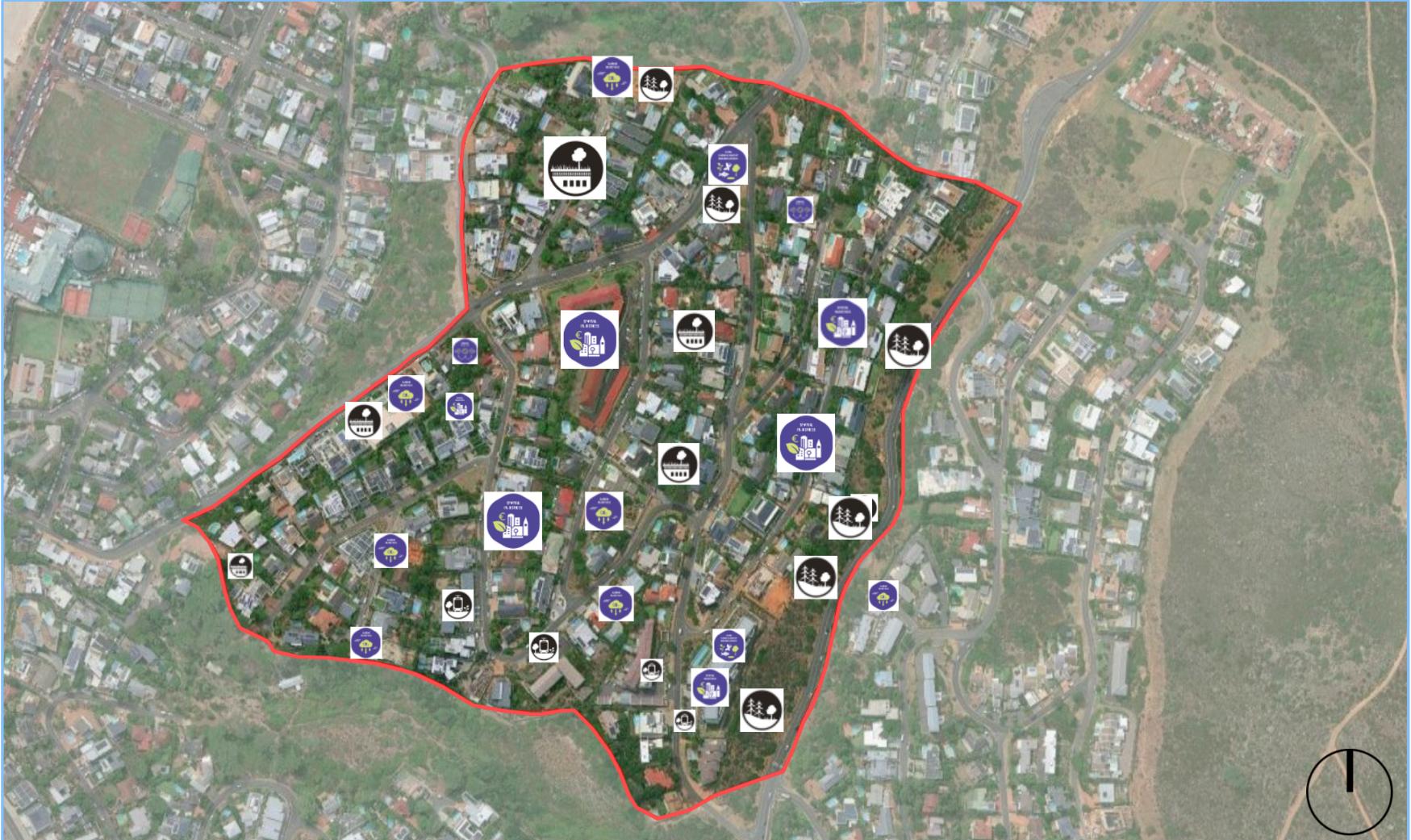
This exercise utilized the JUSTPlanT methodology to map socio-environmental challenges and situate them within a broader territorial context. The process involved identifying existing injustices and activating Nature Based Solutions, analyzing social vulnerability in our selected area from the exercise #4, Camps Bay (Cape Town), and evaluating best practice examples to propose inclusive, climate/resilient interventions. [figure a]
Methods and Data Assumptions
The detailed application of the JUSTPlanT modules resulted in the following spatial and social observations:
● MODULE #1 - Identifying Injustices: We mapped existing injustices at a regional scale, focusing on structural drivers of inequality in Camps Bay
○ Spatial Injustice: Characterized by affluence and exclusivity. The legacy of Apartheid [11] restricts coastal access for low-income groups due to distance and economic barriers.
○ Ecological Injustice: The Marine Protected Area (MPA) suffers from long-term sewage discharge, creating an imbalance where ecosystems degrade while humans benefit from tourism revenues.
● MODULE #2 - Activating NBS: We identified existing and potential Nature Based Solutions, mapping them to respond to the environmental conditions found in Module 1 Many mapped NBS icons [figure a] reflect "ongoing reactive processes" rather than fully implemented solutions. This highlights areas where nature based strategies are already under pressure or only partially functional due to the intense urbanization and environmental stress in the area
● MODULE #3 - Social Inclusiveness: We analyzed social groups most affected by climate pressures (heat, air quality) to ensure NBS prioritizes the most vulnerable.
○ Vulnerable Groups: include the elderly (mobility issues on steep topography), children, pregnant women, and service workers who commute daily and work outdoors.
○ Climate Exposure: High pedestrian activity and unshaded streets increase heat stress.
○ Proposed NBS: Interventions focus on shaded pedestrian routes and accessible resting areas
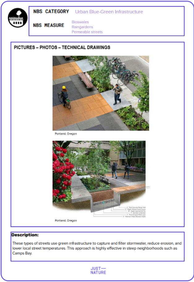
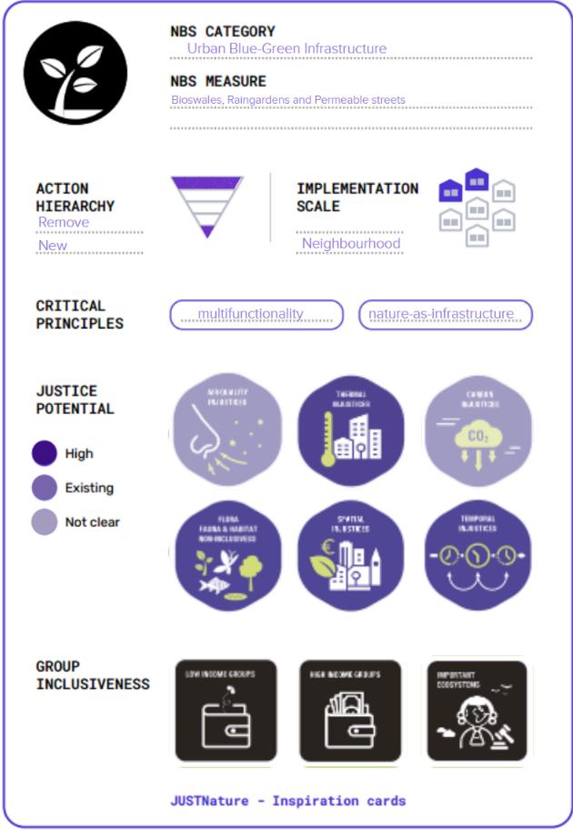
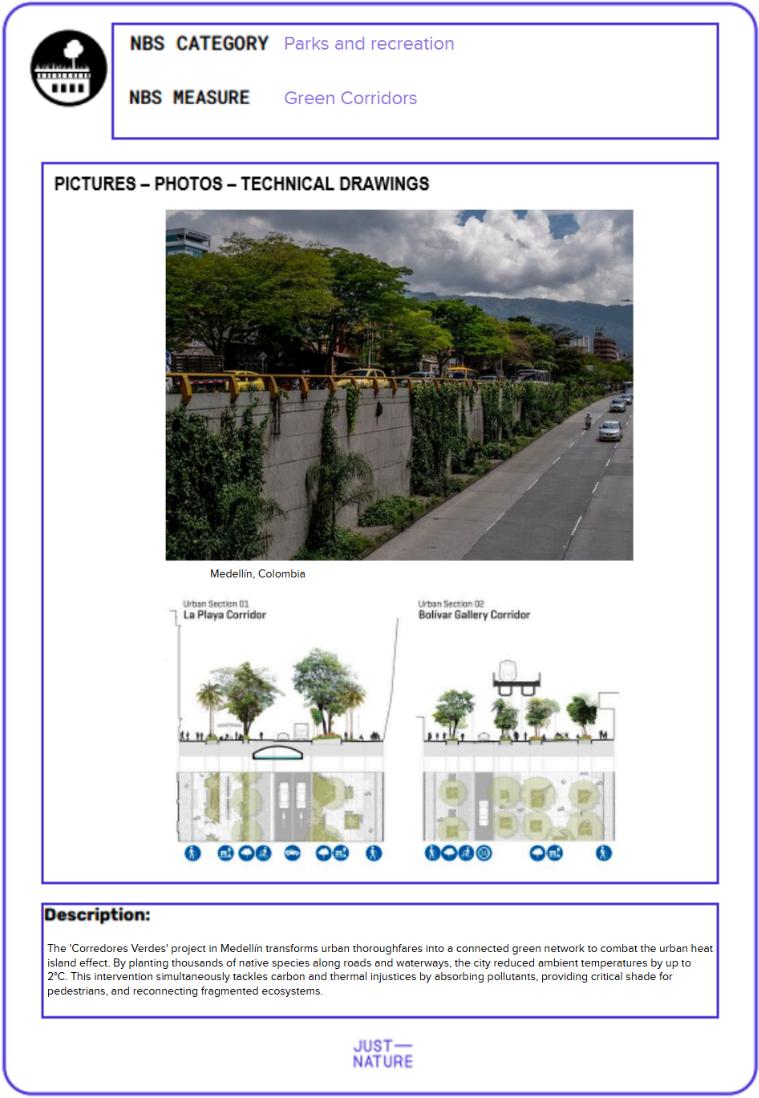
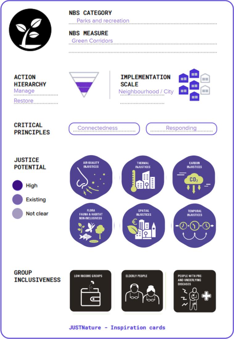
● MODULE #4 - Best Practice Methodology: We followed a structured framework to evaluate an "Inspiration Card" and adapt its principles to the local context [figure b, c, d ,e] . The intervention was defined by action hierarchy (Protect/Restore) and Implementation Scale. We identified critical principles and assessed the "Justice Potential" across six dimensions: Air, Thermal, Carbon, Flora/Fauna, Spatial, Temporal, to address root causes of injustice.
8.1. Critical Analysis and Strategic Implications
The exercise revealed a strong link between spatial injustice, wealth distribution, and Ecological Injustice. In Camps Bay, the degradation of the MPA correlates with prioritizing tourism over ecosystem health. Specific groups face distinct barriers, requiring Nature Based Solutions designed specifically for their needs. Using the JUSTPlanT framework highlighted that true resilience requires shifting from purely technical solutions to socio-ecological interventions that reduce historical inequalities while restoring biodiversity.
9. SIZING A CITY RAIN GARDEN
Methods and Data Assumptions
The local intervention methodology utilizes a simplified calculation model to size city rain gardens by first defining a specific catchment area within the district; analyzed on Exercise #5 of our previous report, Ruyterwacht and Riverton.
The calculation assumes a Composite Runoff Coefficient (C) based on the proportion of covered and uncovered areas. Rainfall depth is determined using an assumed duration of 15 minutes and intensity from local graphs. Final area requirements are calculated using a ponding depth of 150mm, recommended by the teaching materials, and a soil porosity of 0.3.
Calculations and Results
The catchment area; contributing to the runoff, was identified and categorised into permeable and impermeable surfaces to establish the hydrological baseline
Note: The total impermeable area (Roofs + Paved) covers approximately 78.36% of the catchment.
A composite runoff coefficient (C) was calculated using a weighted average based on the surface types. The following coefficients were assumed based on standard.
SUDS References:
➔ C roof = 0 90
➔ C paved = 0.85
➔ C lawn = 0.30
Formula: C = Sum(Ai x Ci) / Total Area
Result: C = [ (20,552 51 x 0 90) + (24,814 72 x 0 85) + (12,556 36 x 0 30) ] / 57,923 59 C ≈ 0 75
This step converts the rainfall depth into a required storage volume and calculates the necessary surface area based on the soil properties and geometry of the garden.
➔ Rain Garden Volume (V) The total volume of water to be managed is the rainfall depth multiplied by the catchment area.
V = Q (converted to m) x Total Area V = 0.01031 m x 57,923.59 m² V ≈ 597.34 m³
➔ Rain Garden Area (Area RG) The area is determined by the vertical capacity of the garden, which includes the ponding depth (surface storage) and the void space in the soil (infiltration storage)
- Soil Porosity (n): 0.30
- Planting Bed Depth (d bed): 0.50 m (Selected to optimize space efficiency)
- Ponding Depth (d pond): 0.15 m
Formula: Area RG = V / [ (n x d bed) + d pond ]
Vertical Capacity: (0.30 x 0.50) + 0.15 = 0.15 + 0.15 = 0.30 m
Result: Area RG = 597.34 / 0.30 Area RG ≈ 1,991.12 m²
To integrate this into the urban design, the total area is divided into 3 separate modules: - Area per module ≈ 664 m² each
DISCIPLINARY REFLECTIONS
Reflecting on the strategic mapping and environmental analysis of our study area, we internalized that environmental resilience is inseparable from ecological justice, as technical performance only succeeds when it addresses the underlying spatial and thermal imbalances within a community. The transition from interpreting national data to carry out viable solutions, taught us that while global data sets the stage, the local priority of actions determine the actual success of an intervention by weighting the protection and restoration of existing natural assets beyond a simple accumulation. We recognized that the most effective nature based solutions are those that move beyond hydraulic efficiency to become living networks that mitigate air pollution and heat stress while providing inclusive space for the most vulnerable urban residents.
As future architects, this study establishes a paradigm shift in our practice where data driven metrics and intellectual capacity become primary tools for advocating high performance landscapes. We now understand that our professional role is not merely to build, but to strategically manage urban challenges through precise technical knowledge to create environments that are both safe and restorative. Our commitment in future projects will be to design with a connected mindset, ensuring that every architectural intervention functions as an equitable asset for human nature across all scales of the city.
ANNEXES
➔ Figure [a] - Potential implementation of NbS
➔ Figures [b, c, d, e] - Inspiration Cards
Card #1 Front
Card #1 Back
Card #2 Front
Card #2 Back
REFERENCES
- [1] UN World Population Prospects 2024 - “South Africa”
- [2] IMF World Economic Outlook Data Mapper - “South Africa”
- [3] World Economic League Table 2024 - “South Africa”
- [4] Mapcarta. “Ruyterwacht.”
- [5] Wikimapia. “Riverton.”
- [6] Texas Department of Transportation. Runoff Coefficients for Urban Watersheds.
- [7] MDPI – Water and Land Journals. Studies on IDF and rainfall–runoff modelling in Mediterranean/subtropical climates.
- [8] Scholz, M., & Grabowiecki, P. “Review of Permeable Pavement Systems.” Water Science and Technology, 2007.
- [9] MDPI – Land. “Infiltration Capacity of Rain Gardens Using Full-Scale Test Method.”
- [10] Urban Drainage and Flood Control District (UDFCD) Urban Storm Drainage Criteria Manual.
- [11] - Refers to the implementation and maintenance of a system of legalized racial segregation in which one racial group is deprived of political and civil rights.
BIBLIOGRAPHY
➢ Yale Center for Earth Observation. (2020). Global Surface Urban Heat Island (UHI) Explorer [Data visualization tool]. Yale University. Retrieved from https://yceo users earthengine app/view/uhimap
➢ World Resources Institute. (2020). Global Forest Watch: Monitoring forests in near real-time [Online platform]. Retrieved from https://www.globalforestwatch.org/
➢ World Health Organization. (2017). Urban green spaces and health: A review of evidence. Geneva: WHO Press. Retrieved from https://www who int/publications/i/item/9789241511345
➢ World Health Organization. (2017). Urban green spaces and health: A review of evidence. Geneva: WHO Press. Retrieved from https://www.who.int/publications/i/item/9789241511345
➢ Bastin, J F , Clark, E , Elliott, T , Hart, S , van den Hoogen, J , Hordijk, I , & Crowther, T. W. (2019). Understanding climate analogs to project future urban climates. PLOS ONE, 14(10), e0214794. https://doi.org/10.1371/journal.pone.0214794
➢ Climate-Data.org. (2021). Climate data for Cape Town (Western Cape, South Africa) [1991–2021 averages]. Retrieved from https://en climate-data org/africa/south-africa/western-cape/cape-town-788/
➢ UN - World Population Prospects 2024. Available at:: https://population.un.org/wpp/
➢ IMF - World Economic Outlook Data Mapper. Available at: https://www.imf.org/external/datamapper/datasets/WEO
➢ CEBR - World Economic League Table 2024. Available at: https://cebr.com/wp-content/uploads/2023/12/WELT-2024.pdf
➢ Our World in Data - CO₂ vs GDP. Available at: https://ourworldindata.org/grapher/co2-emissions-vs-gdp?yScale=log
➢ Bastin, J.F., Clark, E., Elliott, T., Hart, S., van den Hoogen, J., Hordijk, I. & Crowther, T W (2019) Understanding climate analogs to project future urban climates PLOS ONE, 14(10), e0214794. Available at: https://doi.org/10.1371/journal.pone.0214794
➢ CHIRPS Climate Hazards Center (n.d.). Climate Hazards Group InfraRed Precipitation with Station Data. Available at: https://www.chc.ucsb.edu/data/chirps
➢ CIRIA (2015). The SuDS Manual (C753). Construction Industry Research and Information Association, London. Available at: https://www.ciria.org/suds
➢ City of Cape Town (n.d.). Open Data Portal. Available at: https://odp-cctegis.opendata.arcgis.com
➢ Climate Action Tracker (2024). South Africa Country Assessment. Available at: https://climateactiontracker.org/countries/south-africa/
➢ Climate-Data.org (2021). Climate Data for Cape Town, Western Cape, South Africa. Available at: https://en climate-data org/africa/south-africa/western-cape/cape-town-788/
➢ Copernicus Climate Data Store (2024). ERA5 Global Reanalysis Dataset. Available at: https://cds.climate.copernicus.eu
➢ Copernicus Land Monitoring Service (2024). Global Land Cover Viewer. Available at: https://lcviewer.vito.be
➢ ESA DataSpace (2024). Sentinel-2 MSI Satellite Data. Available at: https://dataspace.copernicus.eu
➢ Google Earth Engine (2024). Earth Observation Data Platform. Available at: https://earthengine.google.com
➢ Google Earth Pro (2024) High-resolution Satellite Imagery Available at: https://www.google.com/earth/
➢ Global Forest Watch (2024). Tree Cover, Land Use and Forest Change Data. Available at: https://www.globalforestwatch.org/
➢ NOAA National Centers for Environmental Information (2024). Global Historical Climatology Network Daily (GHCN-D). Available at: https://www.ncei.noaa.gov/products/land-based-station/global-historical-climatologynetwork-daily
➢ OpenStreetMap (2024) Global Collaborative Map Available at: https://www.openstreetmap.org
➢ South African Department of Forestry, Fisheries and the Environment (2023). National Climate Change Adaptation Strategy. Available at: https://www.dffe.gov.za
➢ South African Weather Service (2024) National Rainfall and Climate Records Available at: https://www.weathersa.co.za
➢ Susdrain (2024). Sustainable Drainage Systems Guidance and Case Studies. Available at: https://www.susdrain.org
➢ UNFCCC (2024). South Africa – Nationally Determined Contribution Registry. Available at: https://unfccc int/NDCREG
➢ US Environmental Protection Agency (2024). Green Infrastructure and Low Impact Development. Available at: https://www.epa.gov/green-infrastructure
➢ USGS Earth Explorer (2024). Landsat and Global Surface Data. Available at: https://earthexplorer.usgs.gov
➢ Yale Center for Earth Observation (2020). Global Surface Urban Heat Island Explorer. Available at: https://yceo.users.earthengine.app/view/uhimap