Principles of electronic materials and devices 4th edition kasap solutions manual

Solutions Manual to Principles of Electronic Materials and Devices

Fourth Edition

© 2018 McGraw-Hill CHAPTER 2

Safa Kasap

University of Saskatchewan

Canada

Check author's website for updates

http://electronicmaterials.usask.ca

NOTE TO INSTRUCTORS

If you are posting solutions on the internet, you must password the access and download so that only your students can download the solutions, no one else. Word format may be available from the author. Please check the above website. Report errors and corrections directly to the author at safa.kasap@yahoo.com

A commercial strain gauge by Micro- Measurements (Vishay Precision Group). This gauge has a maximum strain range of ±5%. The overall resistance of the gauge is 350 Ω. The gauge wire is a constantan alloy with a small thermal coefficient of resistance. The gauge wires are embedded in a polyimide polymer flexible substrate. The whole gauge is fully encapsulated in the polyimide polymer. The external solder pads are copper coated. Its useful temperature range is –75 °C to +175 °C.

Copyright © McGraw-Hill Education. All rights reserved. No reproduction or distribution without the prior written consent of McGraw-Hill Education.

(Photo by SK)

Chapter 2

Answers to "Why?" in the text

Page 187, footnote 21

Figure below shows specular reflection, that is, a totally elastic collision of an electron with the surface of a film. If this were a rubber ball bouncing off a wall, then there would only be a change in the ycomponent vy of the velocity, which would be reversed. The x-component is unchanged. The collision has no effect on the vx component of the velocity. If there is an electric field in the x direction then the electron can continue to gain velocity from the field as if it never collided with the wall. Specular reflection does not increase the resistivity.

Page 196, footnote 21

"Pure Al suffers badly from electromigration problems and is usually alloyed with small amounts of Cu, called Al(Cu), to reduce electromigration to a tolerable level. But the resistivity increases. (Why?)" The increase is due to Matthiessen's rule. The added impurities (Cu) in Al provide an additional scattering mechanism.

2.1 Electrical conduction Na is a monovalent metal (BCC) with a density of 0.9712 g cm 3. Its atomic mass is 22.99 g mol 1. The drift mobility of electrons in Na is 53 cm2 V 1 s 1 .

a. Consider the collection of conduction electrons in the solid. If each Na atom donates one electron to the electron sea, estimate the mean separation between the electrons. (Note: if n is the concentration of particles, then the particles’ mean separation d = 1/n1/3.)

b. Estimate the mean separation between an electron (e ) and a metal ion (Na+), assuming that most of the time the electron prefers to be between two neighboring Na+ ions. What is the approximate Coulombic interaction energy (in eV) between an electron and an Na+ ion?

c. How does this electron/metal-ion interaction energy compare with the average thermal energy per particle, according to the kinetic molecular theory of matter? Do you expect the kinetic molecular theory to be applicable to the conduction electrons in Na? If the mean electron/metal-ion interaction energy is of the same order of magnitude as the mean KE of the electrons, what is the mean speed of electrons in Na? Why should the mean kinetic energy be comparable to the mean electron/metal-ion interaction energy?

Copyright © McGraw-Hill Education. All rights reserved. No reproduction or distribution without the prior written consent of McGraw-Hill Education.

d. Calculate the electrical conductivity of Na and compare this with the experimental value of 2.1 × 107 Ω 1 m 1 and comment on the difference.

Solution

a. If D is the density, Mat is the atomic mass and NA is Avogadro's number, then the atomic concentration

is

which is also the electron concentration, given that each Na atom contributes 1 conduction electron. If d is the mean separation between the electrons then d and nat are related by (see Chapter 1 Solutions, Q1.11; this is only an estimate)

b. Na is BCC with 2 atoms in the unit cell. So if a is the lattice constant (side of the cubic unit cell), the density is given by

cell)(mass

cell unit of volume

nm

For the BCC structure, the radius of the metal ion R and the lattice parameter a are related by (4R)2 = 3a2, so that,

If the electron is somewhere roughly between two metal ions, then the mean electron to metal ion separation delectron-ion is roughly R. If delectron-ion ≈ R, the electrostatic potential energy PE between a conduction electron and one metal ion is then

c. This electron-ion PE is much larger than the average thermal energy expected from the kinetic theory for a collection of “free” particles, that is Eaverage = KEaverage = 3(kT/2) ≈ 0.039 eV at 300 K. In the case of Na, the electron-ion interaction is very strong so we cannot assume that the electrons are moving around freely as if in the case of free gas particles in a cylinder. If we assume that the mean KE is roughly the same order of magnitude as the mean PE,

Copyright © McGraw-Hill Education. All rights reserved. No reproduction or distribution without the prior written consent of McGraw-Hill Education.

There is a theorem in classical physics called the Virial theorem which states that if the interactions between particles in a system obey the inverse square law (as in Coulombic interactions) then the magnitude of the mean KE is equal to the magnitude of the mean PE. The Virial Theorem states that:

Indeed, using this expression in Eqn. (2), we would find that u = 1.05 × 106 m/s. If the conduction electrons were moving around freely and obeying the kinetic theory, then we would expect (1/2)meu2 = (3/2)kT and u = 1.1 × 105 m/s, a much lower mean speed. Further, kinetic theory predicts that u increases as T1/2 whereas according to Eqns. (1) and (2), u is insensitive to the temperature. The experimental linear dependence between the resistivity ρ and the absolute temperature T for most metals (non-magnetic) can only be explained by taking u = constant as implied by Eqns. (1) and (2).

d. If µ is the drift mobility of the conduction electrons and n is their concentration, then the electrical conductivity of Na is σ = enµ Assuming that each Na atom donates one conduction electron (n = nat), we have

which is quite close to the experimental value.

Nota Bene: If one takes the Na+-Na+ separation 2R to be roughly the mean electron-electron separation then this is 0.37 nm and close to d = 1/(n1/3) = 0.34 nm. In any event, all calculations are only approximate to highlight the main point. The interaction PE is substantial compared with the mean thermal energy and we cannot use (3/2)kT for the mean KE!

2.2 Electrical conduction The resistivity of aluminum at 25 °C has been measured to be 2.72 × 10 8 Ω m. The thermal coefficient of resistivity of aluminum at 0 °C is 4.29 × 10 3 K 1. Aluminum has a valency of 3, a density of 2.70 g cm 3, and an atomic mass of 27.

a Calculate the resistivity of aluminum at 40ºC

b. What is the thermal coefficient of resistivity at ─40ºC?

c. Estimate the mean free time between collisions for the conduction electrons in aluminum at 25 °C, and hence estimate their drift mobility.

d. If the mean speed of the conduction electrons is about 2 × 106 m s 1, calculate the mean free path and compare this with the interatomic separation in Al (Al is FCC). What should be the thickness of an Al film that is deposited on an IC chip such that its resistivity is the same as that of bulk Al?

e. What is the percentage change in the power loss due to Joule heating of the aluminum wire when the temperature drops from 25 °C to 40 ºC?

Solution

a. Apply the equation for temperature dependence of resistivity, ρ(T) = ρo[1 + αo(T To)]. We have the temperature coefficient of resistivity, αo, at To where To is the reference temperature. We can either work in K or °C inasmuch as only temperature changes are involved. The two given reference temperatures are 0 °C or 25 °C, depending on choice. Taking To = 0 °C,

ρ( 40°C) = ρo[1 + αo( 40°C 0°C)]

ρ(25°C) = ρo[1 + αo(25°C 0°C)]

Divide the above two equations to eliminate ρo,

ρ( 40°C)/ρ(25°C) = [1 + αo( 40°C)] / [1 + αo(25°C)]

Next, substitute the given values ρ(25°C) = 2.72 × 10 8 Ω m and αo = 4.29 × 10 3 K 1 to obtain

b. In ρ(T) = ρo[1 + αo(T To)] we have αo at To where To is the reference temperature, for example, 0° C or 25 °C depending on choice. We will choose To to be first at 0 °C and then at 40 °C (= T2) so that the resistivity at T2 and then at To are:

At T2, ρ2 = ρo[1 + αo(Τ2 Το)]; the reference being To and ρo which defines αo and at To ρo = ρ2[1 + α2(Το Τ2)]; the reference being T2 and ρ2 which defines α2

Rearranging the above two equations we find

α2 = αο / [1 + (Τ2 Τo)αο]

i.e. α 40 = (4 29 × 10 3) / [1 + ( 40 0)(4 29 × 10 3)] = 5 18 × 10 3 °C 1

Alternatively, consider the definition of α2 that is α 40

From oT o o dT d       = ρ ρ α 1

we have α 40 ={1/[ρ( 40 °C)]} × {[ρ(25°C) ρ( 40°C)] / [(25°C) ρ( 40°C)]}

∴ α-40 = 1 / [(2.035 × 10 8)] × {(2 72 × 10 8) (2 035 × 10 8)] / [(25) ( 40)]}

∴ α-40 = 5.18 × 10 3 K 1

c. We know that 1/ρ = σ = enµ where σ is the electrical conductivity, e is the electron charge, and µ is the electron drift mobility. We also know that µ = eτ / me, where τ is the mean free time between electron collisions and me is the electron mass. Therefore,

Copyright © McGraw-Hill Education. All rights reserved. No reproduction or distribution without the prior written consent of McGraw-Hill Education.

Here n is the number of conduction electrons per unit volume. But, from the density d and atomic mass Mat, atomic concentration of Al is

so that n = 3nAl = 1.807 × 10

assuming that each Al atom contributes 3 "free" conduction electrons to the metal and substituting into (1),

(Note: If you do not convert to meters and instead use centimeters you will not get the correct answer because seconds is an SI unit.)

The relation between the drift mobility

mean free time is given by Equation 2.5, so that

d. The mean free path is

where

is the mean speed. With

we find the mean free path:

A thin film of Al must have a much greater thickness than l to show bulk behavior. Otherwise, scattering from the surfaces will increase the resistivity by virtue of Matthiessen's rule.

e. Power P = I2R and is proportional to the resistivity ρ, assuming the rms current level stays relatively constant. Then we have

(Negative sign means a reduction in the power loss).

2.3 Conduction in gold Gold is in the same group as Cu and Ag. Assuming that each Au atom donates one conduction electron, calculate the drift mobility of the electrons in gold at 22° C. What is the mean free path of the conduction electrons if their mean speed is 1.4 × 106 m s 1? (Use ρo and αo in Table 2.1.)

Solution

The drift mobility of electrons can be obtained by using the conductivity relation σ = enµd

Copyright © McGraw-Hill Education. All rights reserved. No reproduction or distribution without the prior written consent of McGraw-Hill Education.

Resistivity of pure gold from Table 2.1 at 0°C (273 K) is ρ0 = 20.50 nΩ m. Resistivity at 20 °C can be calculated by.

The TCR α0 for Au from Table 2.1 is 1/242 K 1. Therefore the resistivity for Au at 22°C is

20.50

Since one Au atom donates one conduction electron, the electron concentration is

Note: The lattice parameter for Au (which is FCC), a = 408 pm or 0.408 nm. Thus l/a = 92. The electron traveling along the cube edge travels for 92 unit cells before it is scattered.

2.4 Mean free time between collisions Let 1/τ be the mean probability per unit time that a conduction electron in a metal collides with (or is scattered by) lattice vibrations, impurities or defects etc. Then the probability that an electron makes a collision in a small time interval δt is δt/τ. Suppose that n(t) is the concentration of electrons that have not yet collided. The change δn in the uncollided electron concentration is then nδt/τ. Thus, δn = nδt/τ, or δn/n = δt/τ. We can integrate this from n = no at x = 0 to n = n(t) at time t to find the concentration of uncollided electrons n(t) at t

n(t) = noexp( t/τ)

Concentration of uncollided electrons [2.85]

Show that the mean free time and mean square free time are given by

What is your conclusion?

Solution Consider

Copyright © McGraw-Hill Education. All rights reserved. No reproduction or distribution without the prior written consent of McGraw-Hill Education.

The last term can be integrated by parts (for example, online at http://www.wolframalpha.com) to find, or in terms of the integration limits, that is, as a definite integral,

Thus, Equation (1) becomes

Now

The definite integral can be evaluated or looked up (for example online at http://www.wolframalpha.com)

Thus Equation (2) becomes,

2.5 Effective number of conduction electrons per atom

a. Electron drift mobility in tin (Sn) is 3.9 cm2 V 1 s 1. The room temperature (20 °C) resistivity of Sn is about 110 nΩ m. Atomic mass Mat and density of Sn are 118.69 g mol 1 and 7.30 g cm 3 , respectively. How many “free” electrons are donated by each Sn atom in the crystal? How does this compare with the position of Sn in Group IVB of the Periodic Table?

b. Consider the resistivity of few selected metals from Groups I to IV in the Periodic Table in Table 2.8. Calculate the number of conduction electrons contributed per atom and compare this with the location of the element in the Periodic Table. What is your conclusion?

Table 2.8 Selection of metals from Groups I to IV in the Periodic Table

NOTE: Mobility from Hall-effect measurements.

Solution

a. Electron concentration can be calculated from the conductivity of Sn, σ = enµd

= 3.70 × 1028 Sn atoms m 3 .

Hence the number of electrons donated by each atom is (ne/nat) = 3.94 or 4 electrons per Sn atom. This is in good agreement with the position of the Sn in the Periodic Table (IVB) and its valency of 4.

b. Using the same method used above, the number of electrons donated by each atom of the element are calculated and tabulated as follows in Table 2Q05.

Table

Copyright © McGraw-Hill Education. All rights reserved. No reproduction or distribution without the prior written consent of McGraw-Hill Education.

2Q05 Number of electrons donated by various elements

As evident from the above table, the calculated number of electrons donated by one atom of the element is the same as the valency of that element and the position in the periodic table.

Table 2Q05 Number of electrons donated by various elements in Excel

2.6 Resistivity of Ta Consider the resisitivity of tantalum, which is summarized in Table 2.9. Plot ρ against T on a log-log plot and find n for the behavior ρ ∝Tn. Find the TCR at 0 and 25 °C. What is your conclusion? (Data from the CRC Handbook of Chemistry and Physics, 96th Edition, 2015-2016)

Table 2.9 Resistivity of Ta

Figure 2Q06-1 shows a plot of resistivity vs. temperature on a log-log plot, from Excel. On a log-log plot, the "best line" is a power law fit on a log-log plot. The best power law fit generates

Copyright © McGraw-Hill Education. All rights reserved. No reproduction or distribution without the prior written consent of McGraw-Hill Education.

y = 0.3642x1.034

R² = 0.9987

*2.7 TCR of isomorphous alloys Determine the composition of the Cu-Ni alloy that will have a TCR of 4×10 4 K 1, that is, a TCR that is an order of magnitude less than that of Cu. Over the composition range of interest, the resistivity of the Cu-Ni alloy can be calculated from ρCuNi ≈ ρCu + Ceff X (1-X), where Ceff, the effective Nordheim coefficient, is about 1310 nΩ m. Solution

Assume room temperature T = 293 K. Using values for copper from Table 2.1 in Equation 2.19, ρCu = 17.1 nΩ m and αCu = 4.0 × 10 3 K 1, and from Table 2.3 the effective Nordheim coefficient of Ni dissolved in Cu is C = 1310 nΩ m. We want to find the composition of the alloy such that αCuNi = 4 × 10 4 K 1. Then,

Using Nordheim’s rule:

Copyright © McGraw-Hill Education. All rights reserved. No reproduction or distribution without the prior written consent of McGraw-Hill Education.

Figure 2Q06-1 Plot of resistivity vs. temperature on a log-log plot. The best line is a power law fit on a log-log plot. (Top, pasted as an editable Excel object, bottom, pasted as bitmap art)

ρalloy = ρCu + CX(1 X)

i.e. 171.0 nΩ m = 17.1 nΩ m + (1310 nΩ m)X(1 X)

∴ X2 X + 0.1175 = 0

solving the quadratic, we find X = 0.136

Thus the composition is 86.4% Cu-13.6% Ni. However, this value is in atomic percent as the Nordheim coefficient is in atomic percent. Note that as Cu and Ni are very close in the Periodic Table this would also be the weight percentage. Note: the quadratic will produce another value, namely X = 0.866. However, using this number to obtain a composition of 13.6% Cu-86.4% Ni is incorrect because the values we used in calculations corresponded to a solution of Ni dissolved in Cu, not vice-versa (i.e. Ni was taken to be the impurity).

Note: From the Nordheim rule, the resistivity of the alloy is ρalloy = ρο + CX(1 X). We can find the TCR of the alloy from its definition

To obtain the desired equation, we must assume that C is temperature independent (i.e. the increase in the resistivity depends on the lattice distortion induced by the impurity) so that d[CX(1 X)]/dT = 0, enabling us to substitute for dρo/dT using the definition of the TCR: αo =(dρo/dT)/ρo. Substituting into the above equation:

Remember that all values for the alloy and pure substance must all be taken at the same temperature, or the equation is invalid.

Comment: Nordheim's rule does not work particularly well for alloys in which one or both elements are transition metals. Its applicability in alloys that involve a transition metal is only approximate as mentioned in the text. The alloy resistivity in these cases is given by

ρalloy = ρCu + CX(1 X) + ρs-d where ρs-d is an additional resistivity term arising from additional scattering mechanism due to the addition of transition metals. This term depends on X2(1 X), which has been neglected. Its inclusion does not dramatically change the results.

2.8 Resistivity of isomorphous alloys and Nordheim’s rule What are the maximum atomic and weight percentages of Cu that can be added to Au without exceeding a resistivity that is twice that of pure gold? What are the maximum atomic and weight percentages of Au that can be added to pure Cu without exceeding twice the resistivity of pure copper? (Alloys are normally prepared by mixing the elements in weight.)

Solution

Cu added Au

Copyright © McGraw-Hill Education. All rights reserved. No reproduction or distribution without the prior written consent of McGraw-Hill Education.

From combined Matthiessen and Nordheim rule, ρAlloy =ρAu + ρI, with ρI = CX(1 X) is the increase in resistivity dues to Cu addition (impurities). In order to keep the resistivity of the alloy less than twice of pure gold, the resistivity of solute (Cu), should be less than resistivity of pure gold, i.e. ρI = CX(1 X) < ρAu. From Table 2.3, Nordheim coefficient for Cu in Au at 20°C is C = 450 nΩ m. Resistivity of Au at 20°C, using α0 = 1/242 K 1 in Table 2.1 is

Therefore the condition for solute (Cu) atomic fraction is ρAlloy =ρAu + ρI < 2ρAu

∴

ρI < ρAu or CX(1 X) < 22.2 nΩ m.

∴ X(1 X) < (22.2 nΩ m) /(450 nΩ m) = 0.0493

Consider the equality case, the maximum Cu addition, X2 – X + 0.0493 = 0

Solving the above equation, we have X = 0.052 or 5.2% (atomic). Therefore the atomic fraction of Cu should be less than 0.052 or 5.2% in order to keep the overall resistivity of the alloy less than twice the resistivity of pure Au. The weight fraction for Cu for this atomic fraction can be calculated from

0.0174 or 1.74% (weight).

Au added to Cu

Now, we discuss the case of Au in Cu, i.e. Au as solute in Cu alloy. Resistivity of Cu at 0°C is 15.4 nΩ m (Table 2.1) and α0 = 1/(235 K). Therefore the resistivity of Cu at 20°C is

Therefore the condition for solute (Au) atomic fraction is ρI = CX(1 X) < ρCu = 17.03 nΩ m. The Nordheim coefficient for Au in Cu at 20°C is, C = 5500 nΩ m. Consider the equality case, the maximum Au addition case,

X(1 X) = (16.71 nΩ m) / (5500 nΩ m) = 3.04×10 3 . X2 – X – 3.04×10 3 = 0

Solving the above equation, we get X = 3.05×10 3 or 0.30 % (atomic) for the maximum Au content we can add. Thus, the Au content has to be less than 0.30% (atomic percent) to keep the resistivity of alloy less than twice of pure Cu. The weight fraction for Cu for this atomic fraction can be calculated from

Copyright © McGraw-Hill Education. All rights reserved. No reproduction or distribution without the prior written consent of McGraw-Hill Education.

9.35 ×10 3 or 0.935% (weight).

2.9 Physical properties of alloys Consider Cu-Sn alloys, called phosphor bronze. Their properties are listed in Table 2.10 from the ASM Handbook. Plot these properties all in graph (using a log-scale for the properties axis) as a function of composition and deduce conclusions. How does κ/σ change? Compositions are wt. %. Assume the Cu-Sn is a solid solution over this composition range.

Table 2.10 Selected properties of Cu with Sn at 20

Note: ρ is resistivity, κ is thermal conductivity, cs is specific heat capacity, λis linear expansion coefficient, E is Young's modulus and d is density.

We can convert wt% to at.% using The atomic fractions of the constituents can be calculated using the relations proved above. The atomic masses of the components are MSn = 118.71 g mol

mol 1.Applying the weight to atomic fraction conversion equation derived in Ch.

for

= 63.54

case

Other values are listed in table 2Q09-1

Copyright © McGraw-Hill Education. All rights reserved. No reproduction or distribution without the prior written consent of McGraw-Hill Education.

Figure 2Q09-1 shows various properties of Cu-Sn alloys as a function of Sn content in atomic percent. Clearly there are strong changes in the electrical resistivity and thermal conductivity whereas cs, λ, E and d are hardly affected at all. The alloy retains metallic bonding, the Cu crystal structure and is a solid solution so there are no major changes in bonding or the crystal structure with up to ~ 5.6 at.% Sn added. The reason both electrical and thermal conductivity are affected strongly is that both depend on the motion of conduction electrons and how these are scattered. The introduction of foreign impurities that provide an additional scattering mechanism increases the resistivity per Matthiessen's rule.

Figure 2Q09-2 shows a plot of the resistivity vs. X(1 X), and it is clearly a straight line with a slope

Slope = C = 1571 nΩ m

This is smaller than the value of C quoted in Table 2.1, which is taken from a handbook (1982).

We can also plot κ vs. σ as in Figure 2Q09-3. Clearly κ is proportional to σ as we expect from the Wiedemann-Franz-Lorenz law. The best fit line passing through the origin and gives a slope of

Slope = CWFLT = 6.862×10 6 so that

CWFL = (6.862×10 6) / (300) = 2.30×10 8 W Ω K 2 .

This value is about 5.7% different than the expected value in Equation 2.42.

NOTE: "Tin bronzes, with up 15.8% tin, retain the structure of alpha copper. The tin is a solid solution strengthener in copper, even though tin has a low solubility in copper at room temperature. The room temperature phase transformations are slow and usually do not occur, therefore these alloys are single phase alloys." From: The Website of the Copper Development Associate (https://www.copper.org/resources/properties/microstructure/cu_tin.html) accessed October 4, 2016

Note: The problem emphasizes the importance of electron scattering in controlling ρ and κ. Normally Cu-Sn phase diagram shows a very small solubility limit for Sn but, as explained above, these compositions are single phase solid solutions.

Copyright © McGraw-Hill Education. All rights reserved. No reproduction or distribution without the prior written consent of McGraw-Hill Education.

Table 2Q09-2 Excel table for the plots

Copyright © McGraw-Hill Education. All rights reserved. No reproduction or distribution without the prior written consent of McGraw-Hill Education.

Figure 2Q09-1 Various properties of Cu-Sn alloys as a function of Sn content.

Figure 2Q09-2 Resistivity vs. X(1 X) for Cu-Sn alloys

2.10 Nordheim’s rule and brass Brass is a Cu–Zn alloy. Table 2.11 shows some typical resistivity values for various Cu–Zn compositions in which the alloy is a solid solution (up to 30% Zn).

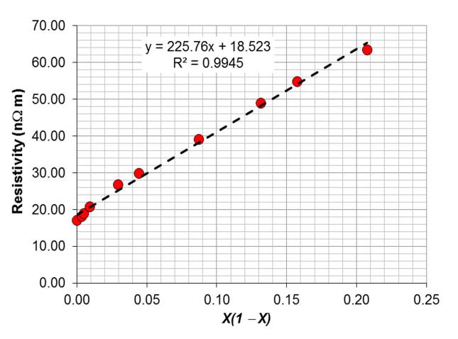
a. Plot ρ versus X(1 X). From the slope of the best-fit line find the mean (effective) Nordheim coefficient C for Zn dissolved in Cu over this compositional range.

b. Since X is the atomic fraction of Zn in brass, for each atom in the alloy, there are X Zn atoms and (1X) Cu atoms. The conduction electrons consist of each Zn donating two electrons and each copper donating one electron. Thus, there are 2(X) + 1(1 X) = 1 + X conduction electrons per atom. Since the conductivity is proportional to the electron concentration, the combined Nordheim-Matthiessens rule must be scaled up by (1 + X).

Plot the data in Table 2.11 as ρ(1 + X) versus X(1 X). From the best-fit line find C and ρo. What is your conclusion? (Compare the correlation coefficients of the best-fit lines in your two plots).

NOTE: The approach in Question 2.10 is an empirical and a classical way to try and account for the fact that as the Zn concentration increases, the resistivity does not increase at a rate demanded by the Nordheim equation. An intuitive correction is then done by increasing the conduction electron concentration with Zn, based on valency. There is, however, a modern physics explanation that involves not only scattering from the introduction of impurities (Zn), but also changes in something called the "Fermi surface and density of states at the Fermi energy", which can be found in solid state physics textbooks.

Copyright © McGraw-Hill Education. All rights reserved. No reproduction or distribution without the prior written consent of McGraw-Hill Education.

Figure 2Q09-3 κ vs. σ for Cu-Sn alloys

Table 2.11 Cu-Zn brass alloys

Data extracted from H. A. Fairbank, Phys. Rev., 66, 274, 1944.

Solution

a. We know the resistivity to be ρalloy = ρo + CX(1-X) and we can construct the table in Table 2Q10-1.

We can now plot ρalloy versus X(1 X). We have a best-fit straight line of the form y = mx + b, where m is the slope of the line. The slope is Ceff, the Nordheim coefficient.

The equation of the line is y = 225.76x + 18.523. The slope m of the best-fit line is 225.76 nΩ m, which is the effective Nordheim coefficient Ceff for the compositional range of Zn provided. b.

Copyright © McGraw-Hill Education. All rights reserved. No reproduction or distribution without the prior written consent of McGraw-Hill Education.

Table 2Q10-1

Figure 2Q10-1: Plot of alloy resistivity against X(1-X)

The slope of the best-fit line is 306.67. As given in the question, the modified combined Nordheim–Matthiessens rule must be scaled up by (1 + X),

The above equation is of the straight line form y = mx +b, where m is the slope of the line. Therefore from the equation of the line y = 306.67x + 17.4, we have the effective Nordheim coefficient is Ceff = 306.67 nΩ m and ρ0 is 17.40 nΩ m.

If we calculate the resistivity using the values obtained above in the combined Nordheim-Mattheisen rule we obtain the following values in Table 2Q10-2

Table 2Q10-2: Ceff values calculated by fitting line to experimental data and by taking into account the effect of extra valence electron

Copyright © McGraw-Hill Education. All rights reserved. No reproduction or distribution without the prior written consent of McGraw-Hill Education.

Figure 2Q10-2: Plot of ρ(1+X) against X(X 1)

For case I, the resistivity is calculated using an effective Nordheim coeffcieint (Ceff) and for the second case the combined Nordheim–Matthiessens rule is scaled up by (1 + X). It is observed that the values obtained by the later method is closer to the experimental results supporting the method of scaling taking into consideration the number of electrons donated by the solute atoms.

Comment: The Nordheim rule assumes that as the alloy composition changes, the number of conduction electrons per metal atom stays the same. In general, the resistivity due to the introduction of solute atoms (impurities) can be written as (see, for example, H. A. Fairbank, Phys. Rev. 66, 274, 1944; see p278.)

where Nat = atomic concentration (roughly constant) and n = average number of conduction electrons per atom. These two terms arise from the fact that scattering from the impurities involves something called the density of states g(EF) which depends on the electron concentration. n will depend on the valency of the solute atom. We can now plot

The plot of ρ vs. X(1 X)/(1+X)2/3 is shown in Figure 2Q10-3. The fit is comparable to the intuitive and classical modification of Nordheim's rule in Figure 2Q10-2.

Copyright © McGraw-Hill Education. All rights reserved. No reproduction or distribution without the prior written consent of McGraw-Hill Education.

2.11 Resistivity of solid solution metal alloys: testing Nordheim’s rule

Nordheim’s rule accounts for the increase in the resistivity from the scattering of electrons from the random distribution of impurity (solute) atoms in the host (solvent) crystal. It can nonetheless be quite useful in approximately predicting the resistivity at one composition of a solid solution metal alloy, given the value at another composition. Table 2.12 lists some solid solution metal alloys and gives the resistivity ρ at one composition X and asks for a prediction ρ ′ based on Nordheim’s rule at another composition X ′ . Fill in the table for ρ ′ and compare the predicted values with the experimental values, and comment.

NOTE: First symbol (e.g., Ag in AgAu) is the matrix (solvent) and the second (Au) is the added solute. X is in at.%, converted from traditional weight percentages reported with alloys. Ceff is the effective Nordheim coefficient in ) (1 0 X X Ceff + = ρ ρ

Solution

Combined Matthiessen and Nordheim rule is

Copyright © McGraw-Hill Education. All rights reserved. No reproduction or distribution without the prior written consent of McGraw-Hill Education.

Figure 2Q10-3: Plot of ρ against X(X 1)/(1+X)2/3

Table 2.12 Resistivities of some solid solution metal alloys

therefore, from the above equation effective Nordheim coefficient Ceff is

For this alloy, it is given that for X = 8.8% Au, ρ = 44.2 n

with ρ0 = 16.2

Ω m, the effective Nordheim coefficient Ceff is

Now, for X′= 15.4% Au, the resistivity of the alloy will be

Similarly, the effective Nordheim coefficient Ceff and the resistivities of the alloys at X′are calculated for the various alloys and tabulated as follows,

Copyright © McGraw-Hill Education. All rights reserved. No reproduction or distribution without the prior written consent of McGraw-Hill Education.

2Q11-1: Resistivities of solid solution metal alloys

Comment: From the above table, the best case has a 0.02% difference and the worst case has a 7% difference. It is clear that the Nordheim rule is very useful in predicting the approximate resistivity of a solid solution at one composition from the resistivity at a known composition.

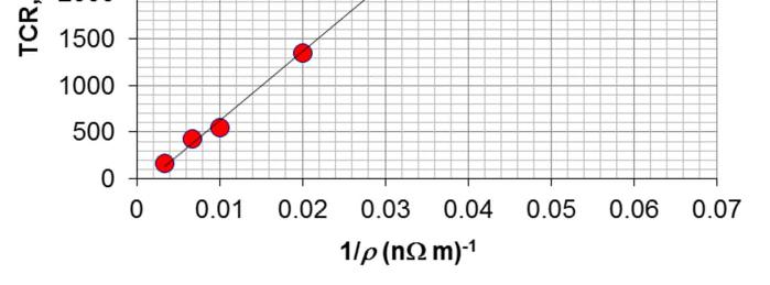
*2.12 TCR and alloy resistivity Table 2.13 shows the resistivity and TCR (α) of Cu–Ni alloys. Plot TCR versus 1/ρ, and obtain the best-fit line. What is your conclusion? Consider the Matthiessen rule, and explain why the plot should be a straight line. What is the relationship between ρCu, αCu, ρCuNi, and αCuNi? Can this be generalized?

Table 2.13 Cu-Ni alloys, resistivity and TCR

NOTE: ppm-parts per million, i.e. 10 6 Solution

We can first construct ta table as shown Table 2Q12-1.

Table 2Q12-1 Resistivity and TCR values

The plot of temperature coefficient of resistivity TCR (α) versus 1/ρ is shown in Figure 2Q12-1, and clearly we can fit a linear relationship with an excellent R2 value, 0.9991. Further, on a log-log plot, shown in Figure 2Q12-2, we can fit a power law dependence of the form

in which n = 1.13, again very close to our expectation 1 alloy alloy ∝ ρ α . Notice that the linear dependence in Figure 2Q12-1 gives a better R2 .

Copyright © McGraw-Hill Education. All rights reserved. No reproduction or distribution without the prior written consent of McGraw-Hill Education.

From Matthiessen’s rules, we have

I o I ρ ρ ρ ρ ρ + = + = matrix alloy where ρo is the resistivity of the matrix, determined by scattering of electrons by thermal vibrations of crystal atoms and ρI is the resistivity due to scattering of electrons from the impurities. Obviously, ρo is a function of temperature, but ρI shows very little temperature dependence. From the definition of temperature coefficient of resistivity,

Copyright © McGraw-Hill Education. All rights reserved. No reproduction or distribution without the prior written consent of McGraw-Hill Education.

Figure 2Q12-1: TCR (α) versus reciprocal of resistivity1/ρ

Figure 2Q12-2: TCR (α) versus reciprocal of resistivity1/ρ on a log-log plot

Clearly the TCR of the alloy is inversely proportional to the resistivity of the alloy. The higher the resistivity, the smaller the TCR, which is evident from the plot.

2.13 Hall effect measurements The resistivity and the Hall coefficient of pure aluminum and Al with 1 at.% Si have been measured at at 20 °C (293 K) as ρ = 2.65 µΩ cm,

3 51×10 11 m3 C 1 for Al and ρ = 3.33 µΩ cm, RH = 3.16×10 11 m3 C 1 for 99 at.% Al-1 at% Si. The lattice parameters for the pure metal and the allloy are 0.4049 nm and 0.4074 nm. What does the simple Drude model predict for the drift mobility in these two metals? How many conduction electrons are there per atom? (Data from M Bradley and John Stringer, J.Phys. F: Metal Phys., 4, 839, 1974)

I. Consider the pure Al crystal

The

We can also find the number x of conduction electrons per Al atom. The atomic concentration in Al is

very close to the valency of Al.

II. Consider the 99%Al-1%Si crystal

We can repeat all the above calculations as follows:

Copyright © McGraw-Hill Education. All rights reserved. No reproduction or distribution without the prior written consent of McGraw-Hill Education.

As expected the drift mobility in this sample is lower due to scattering from Si impurities. We can also find the number x of conduction electrons per Al atom. The atomic concentration in Al is

which is 10% higher than the expected valency.

The lower drift mobility in the Si-1%C crystal is in agreement with the predictions of the Drude model and the Matthiessen's rule.

Note: The Hall coefficient in general is given by

where r is a numerical factor, called the Hall factor, that describes how the electrons are scattered in the crystal. It was taken as 1 in the simple theory above. Generally it is between 1 and 2, and depends on the scattering mechanisms. Unfortunately there is no information on r for the two materials but it should be clear that r would not be the same.

2.14 Hall effect and the Drude model, Table 2.14 shows the experimentally measured Hall coefficient and resisitivities for various metals and their position in the periodic table. (a) Calculate the Hall mobility for each element. (b) Calculate the conduction electron concentration from the experimental value of RH. (c) Find how many electrons per atom are contributed to the conduction electron gas in the metal per metal atom. What is your conclusion?

Note: Data from various sources combined, including C. Hurd, The Hall Coefficient of Metals and Alloys, Plenum, New York, 1972.

Copyright © McGraw-Hill Education. All rights reserved. No reproduction

Table 2.14 Measured Hall coefficients for a few metals at 25 °C

Consider Li, the first element in Group I.

(a) Consider the magnitude of the conductivity product with RH,

The drift mobility µd here is called the Hall mobility

due to the fact that it is found through the product of the Hall coefficient and conductivity.

(b) From the equations for RH, we have

(c) We can get its density and atomic mass from the Appendix at the end of the textbook. If D is the density, Mat is the atomic mass and NA is Avogadro's number, then the atomic concentration

is

We can calculate the number of electrons per Li atom that is in the electron gas as follows

This is close to 1, the valency of Li. The difference is only 11%. Table 2Q14-1 lists the calculations for other elements in Table 2.14.

Conclusions:

The basic idea is "How good is the simple Drude model?"

(1) Group I elements, Li, Na, K, Cs are very close to expected Drude model values with x close to the valency 1; x = 0.89 – 1.10

(2) Group IB, Ag, Cu, Au, have x = 1.18 – 1.47. Although there is a clear deviation from the Drude model by as much as 47%, the sign is correct and the magnitude is very roughly correct, within 47%

(3) Mg, from IIA, has a valency of 2.RH gives x = 1.74 and the difference is only 26%, again the Drude model is not bad.

(4) Zn is a metal and in Group IIB. The Drude model is a total failure as the sign is wrong.

(5) Ca from Group IIA has x = 1.52. The sign is right and the magnitude is very roughly right to within 49%

(6) Group III with Al and In, we find x = 2.33 (In) – 3.05 (Al). The Drude model again is successful in predicting the sign and a rough value for the magnitude, within 67%.

(7) The Drude model works best with Group I elemetns (Li, Na, K, Cs) and in certain cases such as Zn it totally fails.

Table 2Q14-1 Calculations from Hall coefficient and conductivity

Copyright © McGraw-Hill Education. All rights reserved. No reproduction or distribution without the prior written consent of McGraw-Hill Education.

2.15 The Hall effect Consider a rectangular sample, a metal or an n-type semiconductor, with a length

L, width W, and thickness D. A current I is passed along L, perpendicular to the cross-sectional area

WD. The face W × L is exposed to a magnetic field density B. A voltmeter is connected across the width, as shown in Figure 2.40, to read the Hall voltage VH

a. Show that the Hall voltage recorded by the voltmeter is

b. Consider a 1-micron-thick strip of gold layer on an insulating substrate that is a candidate for a Hall probe sensor. If the current through the film is maintained at constant 100 mA, what is the magnetic field that can be recorded per µV of Hall voltage?

Copyright © McGraw-Hill Education. All rights reserved. No reproduction or distribution without the prior written consent of McGraw-Hill Education.

Solution

a. The Hall coefficient, RH, is related to the electron concentration, n, by RH = -1 / (en), and is defined by RH = Ey / (JB), where Ey is the electric field in the y-direction, J is the current density and B is the magnetic field. Equating these two equations:

JB E en y = 1 ∴ en JB E y =

This electric field is in the opposite direction of the Hall field (EH) and therefore:

EH = -Ey = JB en (1)

The current density perpendicular (going through) the plane W × D (width by depth) is:

The Hall voltage (VH) across W is: H H

If we substitute expressions (1) and (2) into this equation, the following will be obtained:

Den IB VH =

Note: this expression only depends on the thickness and not on the length of the sample.

In general, the Hall voltage will depend on the specimen shape. In the elementary treatment here, the current flow lines were assumed to be nearly parallel from one end to the other end of the sample. In an irregularly shaped sample, one has to consider the current flow lines. However, if the specimen thickness is uniform, it is then possible to carry out meaningful Hall effect measurements using the van der Pauw technique as discussed in advanced textbooks.

b. We are given the depth of the film D = 1 micron = 1 µm and the current through the film I = 100 mA = 0.1 A. The Hall voltage can be taken to be VH = 1 µV, since we are looking for the magnetic field B per µV of Hall voltage. To be able to use the equation for Hall voltage in part (a), we must find the electron concentration of gold. Appendix B in the textbook contains values for gold’s atomic mass (Mat =196.97 g mol 1) and density (d = 19.3 g/cm3 = 19300 kg/m3). Since gold has a valency of 1 electron, the concentration of free electrons is equal to the concentration of Au atoms.

Now the magnetic field B can be found by using the equation for the Hall voltage:

Copyright © McGraw-Hill Education. All rights reserved. No reproduction or distribution without the prior written consent of McGraw-Hill Education.

∴ B = 0.0945 T

As a side note, the power (P) dissipated in the film could be found very easily. Using the value for resistivity of Au at T = 273 K, ρ = 22.8 nΩ m, the resistance of the film is:

The power dissipated is then:

2.16 Electrical and thermal conductivity of In Electron drift mobility in indium has been measured to be 6 cm2 V 1 s 1. The room temperature (27 °C) resistivity of In is 8.37 ×10 8 Ωm, and its atomic mass and density are 114.82 amu or g mol 1 and 7.31 g cm 3, respectively.

a. Based on the resistivity value, determine how many free electrons are donated by each In atom in the crystal. How does this compare with the position of In in the Periodic Table (Group IIIB)?

b. If the mean speed of conduction electrons in In is 1.74 ×108 cm s 1, what is the mean free path?

c. Calculate the thermal conductivity of In. How does this compare with the experimental value of 81.6 W m 1 K 1?

a. From σ = enµd (σ is the conductivity of the metal, e is the electron charge, and µd is the electron drift mobility) we can calculate the concentration of conduction electrons (n):

Conclusion: Within the classical theory of metals, this would imply that about three electrons per atom are donated to the conduction-electron sea in the metal. This is in good agreement with the position of the In element in the Periodic Table (III) and its valency of 3.

b. If τ is the mean scattering time of the conduction electrons, then from µd = eτ/me (me = electron mass) we have:

Copyright © McGraw-Hill Education. All rights reserved. No reproduction or distribution without the prior written consent of McGraw-Hill Education.

c. From the Wiedemann-Franz-Lorenz law, thermal conductivity is given as:

This value reasonably agrees with the experimental value.

Note: Indium has a body-centered tetragonal crystal structure and the lattice constants are a = b = 0.325 nm and c = 0.494 nm. The atomic concentration is therefore nat = 2/abc = 3.83 × 1028 m 3, which is the same as nat = dNA/Mat (as we know from Ch. 1).

2.17 Electrical and thermal conductivity of Ag The electron drift mobility in silver has been

measured to be 54 cm2 V 1 s 1 at 27 °C. The atomic mass and density of Ag are given as 107.87 amu or g mol 1 and 10.50 g cm 3, respectively.

a. Assuming that each Ag atom contributes one conduction electron, calculate the resistivity of Ag at 27 °C. Compare this value with the measured value of 1.6 × 10 8 Ω m at the same temperature and suggest reasons for the difference.

b. Calculate the thermal conductivity of silver at 27 °C and at 0 °C.

If we assume there is one conduction electron per Ag atom, the concentration of conduction electrons (n) is 5.862 × 1028 m 3, and the conductivity is therefore:

and the resistivity, ρ = 1/σ = 19.7 nΩ m

The experimental value of ρ is 16 nΩ m. We assumed that exactly 1 "free" electron per Ag atom contributes to conduction. This may not necessarily be true.

Note: More importantly, the difference is part of the failure of classical physics. Some of this will be apparent in Ch. 4 where energy bands are used for conduction.

Copyright © McGraw-Hill Education. All rights reserved. No reproduction

b. From the Wiedemann-Franz-Lorenz law at 27 °C,

For pure metals such as Ag this is nearly independent of temperature (same at 0 °C).

2.18 Mixture rules A 70% Cu - 30% Zn brass electrical component has been made of powdered metal and contains 15 vol. % porosity. Assume that the pores are dispersed randomly. Given that the resistivity of 70% Cu-30% Zn brass is 62 nΩ m, calculate the effective resistivity of the brass component using the simple conductivity mixture rule, Equation 2.26 and the Reynolds and Hough rule. Solution

The component has 15% air pores, which is the dispersed phase. Apply the empirical mixture rule in Equation 2.32. The fraction of volume with air pores is χd = 0.15. Then,

. Substituting the conductivity values in the RHS of the equation we have

Hence the values obtained are the same. Equation 2.32 is in fact the simplified version of Reynolds and Hough rule for the case when the resistivity of dispersed phase is considerably larger than the continuous phase.

2.19 Mixture rules

a. A certain carbon electrode used in electrical arcing applications is 47 percent porous. Given that the resistivity of graphite (in polycrystalline form) at room temperature is about 9.1 µΩ m, estimate the effective resistivity of the carbon electrode using the appropriate Reynolds and Hough rule and the simple conductivity mixture rule. Compare your estimates with the measured value of 18 µΩ m and comment on the differences.

b. Silver particles are dispersed in a graphite paste to increase the effective conductivity of the paste. If the volume fraction of dispersed silver is 30 percent, what is the effective conductivity of this paste?

Copyright © McGraw-Hill Education. All rights reserved. No reproduction or distribution without the prior written consent of McGraw-Hill Education.

a. The effective conductivity of mixture can be estimated using Reynolds and Hough rule in Equation 2.34, which is

If the conductivity of the dispersed medium is very small compared to the continuous phase, as in the given case conductivity of pores is extremely small compared to polycrystalline carbon, i.e.

. Equation 2.32 is the simplified version of Reynolds and Hough rule.

The volume fraction of air pores is χ = 0.47 and the conductivity of graphite is ρc = 9.1 µΩ m, therefore

Conductivity mixture rule is based on the assumption that the two phases α and βare parallel to each other and the effective conductivity from Equation 2.31 is

= 0.47, χgraphite = (1 0.47), σair = 0, σgraphite = (9.1 µΩ m) 1, therefore the effective resistivity using the conductivity mixture rule is

For the given situation

which is not as good as Equation 2.34. We cannot use the resistivity mixture rule. (ρeff goes to inifnity)

b. If the dispersed phase has higher conductivity than the continuous phase, the Reynolds and Hough rule is reduced to Equation 2.33. From Table 2.1, resistivity for silver at 273 K is 14.7 nΩ m. Using α0 = 1/242 K 1, the resistivity at room temperature (20°C) can be calculated as

Since ρd < 0.1ρc, we can try first Equation 2.33 as a first approximation. Volume fraction of dispersed silver is 30%, χd = 0.3. The effective resistivity is

The resisitivity of graphite is therefore reduced i.e. it is made more conducting. This rule works if ρc > ρd/10. Now, ρc = resistivity of graphite = 9.1 µΩ m = 9100 nΩ m from part (a), which is much greater than 16.9 nΩ m for Ag, so the condition is satisfied. Indeed, we did not use ρd at all in this calculation!

In a more accurate calculation, we would use he Reynolds and Hough rule to calculate the effective resistivity. If σ is the effective conductivity (1/ρeff), then

Copyright © McGraw-Hill Education. All rights reserved. No reproduction or distribution without the prior written consent of McGraw-Hill Education.

ρeff = 1/σ = 3.99 µΩ m very close to the approximation in Equation 2.33 Clearly, The approximate equation works well and we did not even need the resistivity of Ag in this case to find the effective resistivity.

2.20 Ag–Ni alloys (contact materials) and the mixture rules Silver alloys, particularly Ag alloys with the precious metals Pt, Pd, Ni, and Au, are extensively used as contact materials in various switches. Alloying Ag with other metals generally increases the hardness, wear resistance, and corrosion resistance at the expense of electrical and thermal conductivity. For example, Ag–Ni alloys are widely used as contact materials in switches in domestic appliances, control and selector switches, circuit breakers, and automotive switches up to several hundred amperes of current. Table 2.15 shows the resistivities of four Ag–Ni alloys used in make-and-break as well as disconnect contacts with current ratings up to ∼100 A.

a. Ag–Ni is a two-phase alloy, a mixture of Ag-rich and Ni-rich phases. Using an appropriate mixture rule, predict the resistivity of the alloy and compare with the measured values in Table 2.15. Explain the difference between the predicted and experimental values.

b. Compare the resistivity of Ag–10% Ni with that of Ag–10% Pd in Table 2.12. The resistivity of the Ag–Pd alloy is almost a factor of 3 greater. Ag–Pd is an isomorphous solid solution, whereas Ag–Ni is a two-phase mixture. Explain the difference in the resistivities of Ag–Ni and Ag–Pd.

Table

NOTE: Compositions are in wt.%. Ag–10% Ni means 90% Ag–10% Ni. d = density and ρ = resistivity. Use volume fraction of Ni = wNi(dalloy/dNi), where wNi is the Ni weight fraction, to convert wt.% to volume %. Data combined from various sources.

Solution

a. The Ni contents are given in wt.%. For volume fraction we use the relation

Copyright © McGraw-Hill Education. All rights reserved. No reproduction or distribution without the prior written consent of McGraw-Hill Education.

2.15 Resistivity of Ag-Ni contact alloys for switches

where wNi is the weight fraction of Ni, dNi is the density of Ni and, d is the density of the alloy mixture. For example, for Ni-30% wt. the volume fraction of Ni in the alloy will be

First we use Reynolds and Hough rule for mixture of dispersed phases to calculate the effective resistivity of the alloy. From Equation 2.28 we have

of the above equation will

Substitute the calculated value in the Reynolds and Hough rule as above, to find the effective resistivity of the alloy, which is ρ = 24.25 nΩ m. Similarly the resistivity of alloy with other Ni contents is calculated and is tabulated below in Table 2Q20-1.

We can see that the Reynolds Hough rule provides a reasonable estimate for the alloy resistivity with the discrepancy being 7.5% at worst case.

Copyright © McGraw-Hill Education. All rights reserved. No reproduction or distribution without the prior written consent of McGraw-Hill Education.

2Q20-1 Resistivity of Ag-Ni contact alloys for switches

b. 90%Ag-10% Ni, the solid is a mixture, and has two phases with an overall ρ = 19.06 nΩ m. On the other hand 90%Ag-10% Pd, the solid is a solid solution with ρ = 59.8 nΩ m, the value is roughly 3 times greater. The resistivity of a mixture is normally much lower than the resistivity of a similar solid solution. In a solid solution, the added impurities scatter electrons and increase the resistivity. In a mixture, each phase is almost like a "pure" metal, and the overall resistivity is simply an appropriate "averaging" or combination of the two resistivities.

Note: Data were extracted from http://www.electrical-contacts-wiki.com

12.21 Ag–W alloys (contact materials) and the mixture rule Silver–tungsten alloys are frequently used in heavy-duty switching applications (e.g., current-carrying contacts and oil circuit breakers) and in arcing tips. Ag–W is a two-phase alloy, a mixture of Ag-rich and W-rich phases. The measured resistivity and density for various Ag–W compositions are summarized in Table 2.16.

a. Plot the resistivity and density of the Ag–W alloy against the W content (wt. %)

b. Show that the density of the mixture, d, is given by

where wα is the weight fraction of phase α, wβ is the weight fraction of phase β, dα is the density of phase α, and dβ is the density of phase β Calculate d and plot it in a above.

c. Show that the resistivity mixture rule is

where ρ is the resistivity of the alloy (mixture), d is the density of the alloy (mixture), and subscripts α and β refer to phases α and β, respectively.

Copyright © McGraw-Hill Education. All rights reserved. No reproduction or distribution without the prior written consent of McGraw-Hill Education.

Figure 2Q20-1 Plot of effective and calculated resistivity for Ni-Ag alloys

d. Calculate the density d and the resistivity ρ of the mixture for various values of W content (in wt. %) and plot the calculated values in the same graph as the experimental values. Try both the resistivity and conductivity mixture rules. What is your conclusion?

Table 2.16 Dependence of resistivity in Ag–W alloy on composition as a function of wt.% W

NOTE: ρ = resistivity and d = density.

Solution

a. The plot of density versus W weight percentage data in Table 2Q21-1, from Table 2.16, is shown in Figure 2Q21-1

Copyright © McGraw-Hill Education. All rights reserved. No reproduction or distribution without the prior written consent of McGraw-Hill Education.

Table 2Q20-1 Resistivity of Ag-W alloys

Alloy

b. The given mixture consists of two phases α, and β. Assume that the total mass of the alloy is Mmixture.

If wα and wβ are the weight fractions of α, and β phases, then their respective masses in the mixture are

The densities of the phases α, and β, are dα and dβ, therefore the volume occupied by these phases can be calculated using the definition of density. i.e. density = mass / volume, we have

The density of the mixture is therefore,

Copyright © McGraw-Hill Education. All rights reserved. No reproduction or distribution without the prior written consent of McGraw-Hill Education.

Figure 2Q21-1: Experimental resistivity and density vs. composition of W in wt%. A simple second order polynomial provides a reasonable fit.

Figure 2Q21-2 shows the experimental and calculated density vs. W (wt. %) points and it is clear that the effective density equation in (1) is quite good in predicting the density over the whole alloy composition.

Figure 2Q21-2 Experimental and calculated density vs. W (wt. %)

c. The resistivity-mixture rule or the series rule of mixtures is defined in Equation 2.30 as

where χα and χβ are the volume fractions of phase α and βrespectively. (For detailed derivation of this rule please see Example 2.14.) Volume fractions of the two phases are,

From part a of this problem, the volume of the phasesα and βin the mixture are

and the volume of the mixture is

V mixture = , therefore the volume fraction of the two contents is

Copyright © McGraw-Hill Education. All rights reserved. No reproduction or distribution without the prior written consent of McGraw-Hill Education.

In summary, the volume fractions are

and χβ, the resistivity mixture rule is

d. We calculate the density and the resistivity using the relations proved in parts b and c. As an example, for 30% W wt. content, the density and resistivity are,

The measured value in Table 2.16 is 12.0 so the calculated value is very close (within 1%).

Using the resistivity-mixture rule, the resistivity of the alloy ρeff is

The experimental resistivity as given in the table is 22.7 nΩ m; difference is only 3.3%. Similarly, the densities and resistivities for the given W contents are calculated and listed in the Table 2Q21-2.

Using the conductivity-mixture rule, the resistivity of the alloy ρeff is

substituting in the values for the RHS

The experimental resistivity 1s given in the table as 22.7 nΩ m; the difference is significant, 16%, especially with respect to the prediction of the series resistivity rule. Clearly the conductivity mixture rule fails.

Similarly, the resistivities for the given W contents are all calculated and listed in the Table 2Q21-2. Figure 2Q21-3 shows the plot of experimental resistivity vs. W content and the resistivities from resistivity and conductivity mixture rules in Equations 2.30 and 2.31 respectively.

Copyright © McGraw-Hill Education. All rights reserved. No reproduction or distribution without the prior written consent of McGraw-Hill Education.

Major assumption: Ag-W is a two phase alloy, made up of α (Ag-rich) and β(W-rich) phases. We assumed that we can simply use the properties of Ag for the α and the properties of W for the βphase.

Comment: The data were collected from a variety of sources (various handbooks and papers) and combined into a single table. The data are not simply from a single source. Hence the experimental values show some scatter.

Copyright © McGraw-Hill Education. All rights reserved. No reproduction or distribution without the prior written consent of McGraw-Hill Education.

Figure 2Q21-3 Experimental resistivity and resistivities from resistivity and conductivity mixture rules vs. W (wt. %)

Table 2Q21-2: Resistivity of Ag–W alloy as a function of wt.% W calculated using series mixture and parallel mixture rules.

Given the scatter, the resistivity mixture model is in very good agreement with the experimental data. The conductivity mixture rule fails badly in this case.

2.22 Strain gauges Consider a strain gauge that consists of a nichrome wire of resistivity 1100 nΩ m, TCR (α) = 0.0004 K 1, a total length of 25 cm, and a diameter of 50 µm. What is δR for a strain of 10 3? For nichrome, ν ≈ 0.3. What is δR if there is a temperature variation of 1 °C, given that the linear thermal expansion coefficient is 15 ppm K 1?

Solution

Clearly we can easily measure the strain through δR, which is roughly 2 Ω; although a temperature fluctuation can significantly affect the measurement. Indeed, we need to compensate for the temperature fluctuation effects, otherwise the changes in δR will not reflect the changes in the strain. See Question 2.23

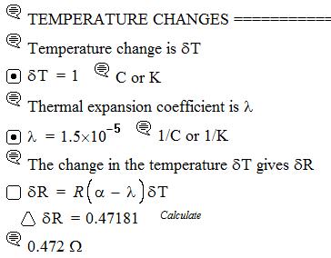
Comment: λ= 14 ppm/K is typical of nichrome wires

2.23 Strain measurements How would you use strain gauges in a Wheatstone bridge circuit to measure strains and reduce the effects of temperature variations? What would be the advantages and disadvantages of such a bridge circuit?

Solution

Copyright © McGraw-Hill Education. All rights reserved. No reproduction or distribution without the prior written consent of McGraw-Hill Education.

Figure 2Q23-1a shows a Wheatstone bridge. In Figure 2Q23-1b, R4 is the strain gauge, represented as Rs. The voltage between the terminals b and a is given by

so that the normalized voltage v between b and a is

Figure 2Q23-1 Wheatstone bridge configurations for measuring strain.

I. Strain measurement without temperature compensation, and R4 as the strain gauge Rs

Take R4 = Rs, the strain gauge. A small change in Rs gives a change in v,

The fractional change in the voltage δv per unit fractional change in Rs is the sensitivity S, that is,

Representing the ratio Rs/R3 = x, we have

Copyright © McGraw-Hill Education. All rights reserved. No reproduction or distribution without the prior written consent of McGraw-Hill Education.

This quantity represents how the sensitivity S of the bridge depends on Rs/R3 = x as shown in Figure 2Q23-2. Clearly, S has a maximum magnitude at x = 1, that is, when Rs = R4 = R3 and it is S = 0.25

Consider a strain gauge with a gauge factor (GF) of 1.6 (see Example 2.13), V = 10 V and Rs = 1000 Ω. What is the signal for a strain of 0.1%?

V = (10 V)(0.4×10

) = 0.004 V or 4 mV, which is measurable Note that the responsivity (δV) can be increased by using a higher V across the bridge. 20 V would give a voltage change of 8 mV.

II. Temperature compensation

In this case, we need to compensate for the change in R4 with temperature. If an exactly identical strain gauge is used for R3 (which is called a reference gauge Rref) but only R4 is subject to the strain, and both are subject to the same temperature change, then δV will not be affected by a temperature variation. The circuit is shown in Figure 2Q23-1c. Consider

Assume R1 = R2, R3 = R4 (for maximum bridge sensitivity). For a temperature change δT, δR1 = δR2 and δR3 = δR4 so that we always have v = 0.

However, the strain only affects R4 and not R3. The derivation in Part I is valid and

Advantages

1. In a Wheatstone bridge sensing circuit, one is measuring changes about zero volts across the bridge between a and b in Figure 2Q23-1b.

Copyright © McGraw-Hill Education. All rights reserved. No reproduction or distribution without the prior written consent of McGraw-Hill Education.

Figure 2Q23-2 Sensitivity vs. x = R3/Rs