
Solution Manual for The Basic Practice of Statistics, 8th Edition, David S. Moore
Full download chapter at: https://testbankbell.com/product/solution-manualfor-the-basic-practice-of-statistics-8th-edition-david-s-moore/
Chapter 1 –
Picturing Distributions with Graphs
1.1 (a) Theindividualsarethecarmakesandmodels. (b) Foreachindividual,the variablesrecordedare:vehicleclass(categorical),transmissiontype(categorical), numberofcylinders(usuallytreatedasquantitative),citympg(quantitative), highwaympg(quantitative),andannualfuelcostindollars(quantitative).
1.2 Answerswillvary Somepossiblecategoricalvariables:whetherornotthe studentplayssports;sex;whetherornotthestudentsmokes;andattitudeabout exercise.Somepossiblequantitativevariables:weight(kilogramsorpounds),height (centimetersorinches);restingheartrate(beatsperminute);andbodymassindex (kg/m2 orlb/ft2).
1.3 (a) 91%usethesetopsocialmediasites;9%useothersitesmostoften. (b) A bargraphisprovided.
(c) Ifyouincludean “Other”category,thenapiechartisappropriate.Thissurvey askedaboutthesiteusedmostoften,soeachindividualisonlyrepresentedinone category,andthecategoriesmakeupthewhole.
1.4 (a) Individualsfallintomorethanoneofthecategories. (b) Abargraphis shown.

1.5 Apiechartcanbemadebecausethedaysarenon-overlappingandmakeupthe whole.Somebirthsarescheduled(inducedlabor,forexample)and,probably,most arescheduledforweekdays.
1.6 Makethishistogrambyhand,astheinstructionssuggest.
1.7 Usetheapplettoanswerthesequestions.
1.8 Thedistributionisslightlyright-skewed.Thecenterisbetween30%and40% (23stateshavelessthan30%minorityresidents,andanother10stateshave between30%and40%).Thestatewidepercentsrangefromabout0%toabout 80%.Nostateshaveanunusuallylargeorsmallpercentofminorityresidents.

1.9 (a) Therearetwoclearpeaksinthedistribution.Ifwegaveonlyonecenter,it wouldmostlikelybebetweentheseandnotbetrulyrepresentative. (b) Youngboys mightspendalotoftimeoutdoorsplaying;theirtimeoutsideinplaceswherethey wouldencounterticksmightwellbelessinyoungeradulthood.Withfamiliesand yardwork,theirtimeoutsidemightincrease. (c) No,thisisincorrect.Hikinginthe woodsatanyagewillmakeapersonmorelikelytoencountertheticksthatspread Lymedisease. (d) Thehistogramshavethesameshapes,butfemaleshaveaslightly lowerincidencerateuntilage65,afterwhichfemaleshaveaslightlyhigherrate. Femalesunderage65,possibly,spendlesstimeoutdoorsinareaswheretheywould encounterticks.

1.10 (a) Astemplotisprovided.Withasinglestem,thedistributionappeared unimodal.Aftersplittingthestems,itappearsbimodal.
(b) Thehistogramwithbinsofwidth5willgivethesamepatternasthestemplot frompart(a).

1.11 Hereisastemplotforhealthexpenditurepercapita(inPPP).Dataarerounded tounitsofhundreds.Forexample,Argentina’s1725becomes17.Stemsare thousandsandaresplit,asprescribed Thisdistributionisright-skewed,witha singlehighoutlier(UnitedStates).Thereseemtobetwoclustersofcountries.The centerofthisdistributionisaround20($2000spentpercapita).Thedistribution variesfrom0|2(about$200spentpercapita)to9|1(about$9100spentpercapita).
1.12 (a) Atimeplotofaveragetuitionandfeesisgiven.
(b) Averagetuitionandfeeshavesteadilyclimbedduringthe35-yearperiod,with sharpestabsoluteincreasesbetween2009and2012. (c) Averagetuitionandfees havenotdecreased(asshowninthisplot),buttherehavebeenperiodsofvery smallincreases(1995–2000and2012–2013,forexample).Therearetwoperiodsof veryrapidincreases:2000–2005and2008–2012. (d) Itwouldbebettertouse percentincreasesratherthandollarincreases.A10%increaseinaveragetuition
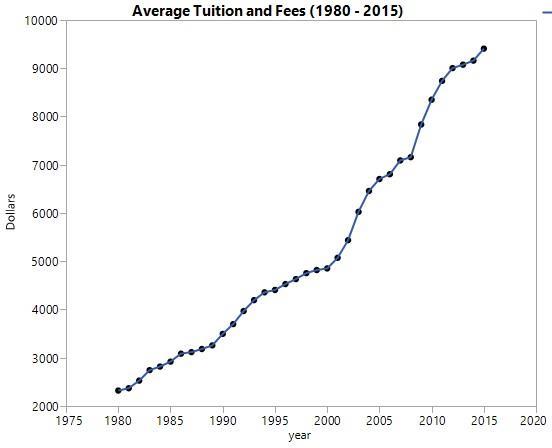
andfeesin1980shouldcorrespondtoa10%increaseinaveragetuitionandfeesin 2005,buttheabsolutedollarincreasesinthesecasesareverydifferent.
1.13 (a)thestudents.
1.14 (c)abargraphbutnotapiechart.Individualscouldbelongtomorethanone category.
1.15 (b)Squarefootageandaveragemonthlygasbillarebothquantitative variables.
1.16 (b)categoricalvariable.Zipcodesareequivalenttotown(orzone)namesor identifications,andyoucan’tdoarithmeticmeaningfullywiththem.
1.17 (b)88%to92%.
1.18 (b)2,3,4,5,6,7,8,9.
1.19 (b)76%.Thereare50observations,sothecenterwouldbebetweenthe25th and26th observations;bothoftheseare76%.
1.20 (a)skewedtotheleft.
1.21 (c)34%enrolled.Thestemsareroundedtowholepercents;youcannotmake finerjudgments.
1.22 (c)skewedtotheright.
1.23 (a) Individualsarestudentswhohavefinishedmedicalschool. (b) Five,in additionto“Name.”“Age”(inyears)and“USMLE”(inscorepoints)arequantitative. Theothersarecategorical.
1.24 ThecategoricalvariablesarefreezertypeandEnergyStarcompliant(yes/no). Thequantitativevariablesareannualenergyconsumption(kw),width(in),depth (in),height(in),freezercapacity(ft3),andrefrigeratorcapacity(ft3).Theindividuals aretherefrigeratormakesandmodels.
1.25 “Othercolors”shouldaccountfor2%.Abargraphwouldbeanappropriate display.Ifyouincludedthe“Other”category,apiechartcouldalsobemade.
1.26 (a) Abargraphforthepercentwhousedanytobaccoproductisgiven.The percentstayedrelativelyconstant,withaslightdecreasefrom2011to2013and increasingsince.

(b) Seethebarchartgiven.
(c) Theplotinpart(b)showsthattherecentincreaseintobaccousageisduetoa drasticincreaseintheuseofe-cigarettes.Usageofotherformsoftobaccohas decreasedsince2011.

1.27 (a) Abargraphisgiven
(b) Yes,wecanconstructapiechartifweprovidean"Other"category,wherethe totalnumberofdeathsinthe"Other"categoryis28486-11619-4878-4329-14961170-362=4632.Thecreationofan"Other"categoryisrequiredforapiechartso thatthenumberofdeathsineachsubcategorysumtothetotalnumberofdeaths. Withoutan"Other"category,wecannotconstructapiechart.
1.28 About20%haddebtbetween$25,000and$49,999.Lessthan5%haddebt above$150,000,butitishardtotellfromtheplot.
1.29 (a) Abargraphisprovided.
(b) Forthe18–34agegroup,thehoursareroughlyequal.Fortheolderagegroups, socialappsareusedmoreoftenthanentertainmentapps (c) Apiechartisnot appropriatebecausethesedatadonotrepresentallpartsofawhole.

1.30 Thisdistributionisright-skewed,withthecenteraroundtwoservingsanda variabilityofzerotoeightservings.Therearenooutliers.About12%(9outof74) consumedsixormoreservings,andabout35%(26outof74)atefewerthantwo servings(zerooroneserving).
1.31 (a) Ignoringthefourloweroutliers,thedistributionisroughlysymmetric,is centeredatascoreof111,andhasarangeof86to136. (b) 62ofthe78scoresare morethan100.Thisis79.5%.
1.32 (a) Thedistributionisslightlyleft-skewed(somemightcallitalmost symmetric). (b) Thecenterissomewherebetween0%and2.5%. (c) Thesmallest valueissomewherebetween–12.5%and–10%,andthelargestvalueisbetween 125%and15%. (d) Thereareabout140negativereturns,althoughyourestimate coulddiffer.Thiscorrespondstoabout38%.
1.33 (1.) “Areyoufemaleormale?”isHistogram(c).Therearetwooutcomes possible,andthedifferenceinfrequenciesislikelytobesmallerthantherighthanded/left-handeddifferenceinpart(2). (2.) “Areyouright-handedorlefthanded?”isHistogram(b),sincetherearemoreright-handedpeoplethanlefthandedpeople,andthedifferenceislikelylargerthanthesexdifferenceinpart(1). (3.) “Whatisyourheightininches?”isHistogram(d).Heightdistributionislikelyto besymmetric. (4.) “Howmanyminutesdoyoustudyonatypicalweeknight?”is Histogram(a).Thevariabletakesonmorethantwovalues,andtimespentstudying maywellbearight-skeweddistribution,withmoststudentsspendinglesstime studying,butsomestudentsstudyingalot.
1.34 (a) Ahistogramisprovided.
(b) Thisisanextremelyright-skeweddistribution.Ratiosgreaterthan1correspond toanoilwithmoreomega-3thanomega-6 Thisaccountsfor7ofthe30oils,or 23.3%.Mostfoodoilsaren’tthishealthy. (c) Ofthe7healthierfoodoils,5come fromtypesoffish.Furthermore,allofthefishoilsinthelisthaveratioshigherthan 1 Clearly,fishoilsprovideahealthierratioofomega-3toomega-6acids.
1.35 (a) Statesvaryinpopulation,soyouwouldexpectmorenursesinCalifornia thaninWyoming,forexample.Nursesper100,000providesabettermeasureofthe numberofnursesavailabletoserveastate’spopulation. (b) Astemplotisprovided. Roundthedatatothenearestten,andusethestemsforhundredsandtheleavesfor tens.Thedistributionisslightlyleft-skewed,withacenteraround900andarange from590to1480nursesper100,000.Theobservationwith1480nursesisan outlier.ThiscorrespondstoWashingtonD.C.;manypeopleliveinstates surroundingD.C.butcommutetoD.C.tohealthcare.
Stem Leaf
10 0122234599
9 001113455578
8 001133556668
7 246
6 11347889
5 9
(c) Splittingthestemswouldbeuseful,becauseitwouldbetterallowyoutoseethe variabilitybetweenthelargenumberofstateswithbetween800and1100nurses per100,000.
1.36 (a) Becausethecountrieshavevaryingpopulations,comparingthembydeaths per1000childreniseasierthanbytotalnumberofchildren. (b) Thehistogramis provided Thedistributionisright-skewed,withacenteraround20deathsper1000 children.Therangeisfromjustabove0to160.Angolamaybeconsideredan outlier,withadeathrateofabout160.
1.37 Thestemplot(afterroundingtothenearestthousand)isshown.Theshapeof thedistributionisroughlysymmetric(itmightbecalledleft-skewedifweignorethe highoutlier);withthisscaling,245seemstobeahighoutlier Thecenterisabout 171(the12thobservation).Thedatarangefromabout91toabout245.

1.38 (a) Anegativevaluemeansthatthevirtual operationtooklongerafterthe four-weekprogramthanittookbeforetheprogram. (b) Thestemplotisprovided.
(c) Thecenterforthetreatmentgroupisabout130seconds;forthecontrolgroup, thecenterisabout60seconds.Itappearsthatthetreatmentgrouphadlarger differences,sohadgreaterimprovement.
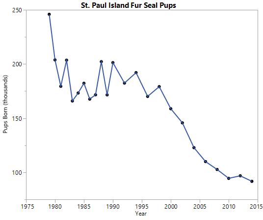
1.39 Atimeplotoffursealpups.Thedeclineinpopulationisnotseeninthe stemplotmadeinExercise1.37.
1.40 (a) Ratesareappropriate(ratherthannumbersofaccidents)becausethe groupsizesaredifferent.Ifmarijuanadidnotincreasewiththerateofaccidents, thenyouwouldstillhavemoreaccidents(bycount)inthelargestgroups. (b) The rateswerecomputedasaccidents/(numberofdrivers)ineachgroup;abargraph isgiven.Whilewecannotconcludethatmarijuanausecausesaccidents,itis certainlyassociatedwithagreateraccidentrate.Perhapsthe“risktaking”aspect mentionedmightalsobeanexplanation.
1.41 (a) Abargraphisprovided.Threeseparatebargraphscouldalsohavebeen produced.


(b) Allcountriesspendmuchmoretimeoneitheradesktoporasmartphoneapp

TheU.S.usessmartphoneappsmorethandesktops,whichisnottrueforCanada andtheU.K. (c) Apiechartcanbeconstructedbecausewithineachcountry,thefive categorieslistedcoverallpossiblechoicesofaccessmethod,withthesumofthe percentsbeing100 Comparingthedistributionsacrosscountryiseasierwiththe side-by-sidebargraphbecausethebarsaregroupedbyaccessmethod.


1.42 (a) Herearestemandsplit-stemplots.Inbothcases,stemsdenotethetens place.
(b) Thecenterofthisdistributionisaround62correctidentifications;thedatavary from49to70 Thedistributionissomewhatleft-skewed Therearenooutliers. (c) Itwouldappearthataperson’svoicedoeshelpidentifythetallerperson.If subjectswerejustguessing,wewouldexpectthedistributiontocenterabout50, butthecenterhereismuchhigher.Infact,onlyonepersoncorrectlyidentifiedthe tallerpersonlessthan50times,andthatwas49correct.
1.43 (a) Graph(a)appearstoshowthegreatestincrease.Verticalscalingcan impacttheperceptionofthedata. (b) In2000,tuitionwasabout$5000,anditrose toabout$9500in2015;thisisanincreaseofapproximately$4500.Bothplots describethesamedata.
1.44 (a) Thetimeplotsareprovided Thepatternsaresimilar,butthechangesin unemploymentratearemuchlessdrasticforcollegegraduatesthanforhighschool graduates.
(b) Thefinancialcrisisof2008isobservedintheplotbyasharpincreasein unemploymentratesin2008and2009.Since2009,unemploymentrateshave steadilydecreased,almostbacktothelevelsseenbeforethefinancialcrisis. (c) A slightincreaseinunemploymentratescanbeseenbeginningin2001.
1.45 (a) Itseemsasthoughwinterquartersaretypicallyassociatedwithlower housingstarts. (b) and (c) Overthelongrunhousingstartshaverisen,exceptfor

crisisyears,whichareshownbythesharpdecreasebetween2005and2008. (d) Since2011,itappearsthathousingstartsareagainincreasingfromyeartoyear
1.46 Usethe One-Variable Statistical Calculator appletonthetextwebsiteto investigatethisproblem.