Download pdf Ai and machine learning for on-device development: a programmer's guide 1st edition mor
Visit to download the full and correct content document: https://ebookmeta.com/product/ai-and-machine-learning-for-on-device-development-a -programmers-guide-1st-edition-moroney/
More products digital (pdf, epub, mobi) instant download maybe you interests ...
Applied Machine Learning and AI for Engineers Jeff
With Early Release ebooks, you get books in their earliest form— the author’s raw and unedited content as they write—so you can take advantage of these technologies long before the official release of these titles.
Published by O’Reilly Media, Inc., 1005 Gravenstein Highway North, Sebastopol, CA 95472.
O’Reilly books may be purchased for educational, business, or sales promotional use. Online editions are also available for most titles (http://oreilly.com). For more information, contact our corporate/institutional sales department: 800-998-9938 or corporate@oreilly.com.
Acquisitions Editor: Rebecca Novack
Development Editor: Jill Leonard
Production Editor: Daniel Elfanbaum
Interior Designer: David Futato
Cover Designer: Karen Montgomery
Illustrator: Kate Dullea
December 2021: First Edition
Revision History for the Early Release
2021-04-22: First Release
2021-06-18: Second Release
See http://oreilly.com/catalog/errata.csp?isbn=9781098101749 for release details.
The O’Reilly logo is a registered trademark of O’Reilly Media, Inc. AI andMachineLearningOn-DeviceDevelopment, the cover image, and related trade dress are trademarks of O’Reilly Media, Inc.
The views expressed in this work are those of the authors, and do not represent the publisher’s views. While the publisher and the authors have used good faith efforts to ensure that the information and instructions contained in this work are accurate, the publisher and the authors disclaim all responsibility for errors or omissions, including without limitation responsibility for damages resulting from the use of or reliance on this work. Use of the information and instructions contained in this work is at your own risk. If any code samples or other technology this work contains or describes is subject to open source licenses or the intellectual property rights of others, it is your responsibility to ensure that your use thereof complies with such licenses and/or rights.
978-1-098-10168-8
[FILL IN]
Chapter 1. Introduction to AI and Machine Learning
A NOTE FOR EARLY RELEASE READERS
With Early Release ebooks, you get books in their earliest form— the author’s raw and unedited content as they write—so you can take advantage of these technologies long before the official release of these titles.
This will be the 1st chapter of the final book. The GitHub repo is https://github.com/lmoroney/odmlbook.
If you have comments about how we might improve the content and/or examples in this book, or if you notice missing material within this chapter, please reach out to the editor at jleonard@oreilly.com.
You’ve likely picked this book up because you’re curious about Artificial Intelligence (AI), Machine Learning (ML), Deep Learning and all of the new technologies that promise the latest and greatest breakthroughs. Welcome! In this book, my goal is to explain a little about how AI and ML work, and a lot about how you can put them to work for you in your mobile apps using technologies such as TensorFlow Lite, ML Kit and CoreML. We’ll start light, in this Chapter, by establishing what we actually meanwhen we describe Artificial intelligence, Machine Learning, Deep Learning and more.
What is Artificial Intelligence?
In my experience, Artificial Intelligence, or AI, has become one of the most fundamentally misunderstood technologies of all time.
Perhaps the reason for this is in its name -- Artificial Intelligence evokes the artificialcreation of an intelligence.Perhaps it’s in the use of the term widely in science fiction and pop culture, where AI is generally used to describe a robot that looks and sounds like a human. I remember the character Data from StarTrek:TheNext Generation, as the epitome of an Artificial Intelligence, and his story led him in a quest to be human, because he was intelligent and selfaware, but he lacked emotions. Stories and characters like this have likely framed the discussion of Artificial Intelligence. Others, such as nefarious AIs in various movies and books have led to a fear of what AI can be.
Given how often AI is seen in these ways, it’s easy to come to the conclusion that they define AI. However, none of these are actual definitions or examples of what Artificial Intelligence is, at least in today’s terms. It’s not the artificial creation of intelligence -- it’s the artificial appearanceof intelligence. When you become an AI developer, you’re not building a new lifeform -- you’re writing code that acts in a different way to traditional code, and that can very loosely emulate the way an intelligence reacts to something. Common areas of these are to use deep learning for Computer Visionwhere, instead of you writing code that tries to understand the contents of an image with a lot of if..then rules that parse the pixels,, you can instead have a computer learnwhat the contents are by ‘looking’ at lots of samples.
So, for example, say you want to write code to tell the difference between a tee-shirt and a boot. (Figure 1-1)
How would you do this? Well, you’d probably want to look for particular shapes. The distinct vertical lines in parallel on the tee shirt, with the body outline, are a good signal that it’s a tee shirt. The thick horizontal lines towards the bottom, the sole, are a good
Figure 1-1. ATee Shirtanda Boot
indication that it’s a boot. But there’s a lot of code you would have to write to detect that. And that’s just for the general case -- of course there would be many exceptions for non-traditional designs, such as a cut-out tee shirt.
If you were to ask an intelligent being to pick between a shoe and a tee shirt, how would you do it? Assuming it had never seen them before, you’d show the being lots of examples of boots, and lots of examples of tee shirts, and it would just figure out what made a boot a boot, and what made a tee shirt a tee shirt. You wouldn’t need to give it lots of rulessaying which one is which. Artificial Intelligence acts in the same way. Instead of figuring out all those rules, and inputting them into a computer in order to tell that difference, you give the computer lots of examples of tee shirts, and lots of examples of shoes, and it just figures out how to distinguish them.
But the computer doesn’t do this by itself. It does it with code that you write. That code will look and feel verydifferent from your typical code, and the framework by which the computer will learn to distinguish isn’t something that you’ll need to figure out how to write for yourself. THere are several frameworks that already exist for this purpose. In this book you’ll learn how to use one of them, TensorFlowto create applications like the one I just mentioned!
TensorFlow is an end-to-end open source platform for ML. You’ll use many parts of it extensively in this book, from creating models that use ML and deep learning, to converting them to mobile-friendly formats with TensorFlow Lite and executing them on mobile devices, to serving them with TensorFlow-Serving. It also underpins technology such as ML Kit, which brings many common models as turnkeyscenarioswith a high level API that’s designed around mobile scenarios.
As you’ll see when reading this book, the techniques of AI aren’t particularly new or exciting. What isrelatively new, and what made
the current explosion in AI technologies possible is increased, lowcost computing power, along with the availability of mass amounts of data. Having both of these is key to building a system using Machine Learning. But to demonstrate the concept, let’s start small, so it’s easier to grasp.
What is Machine Learning?
You might have noticed, in the above scenario, that I mentioned that an intelligent being would look at lots of examples of tee shirts and boots and just figure out what the difference between them was, and in so doing, would learnhow to differentiate between them. It had never previously been exposed to either, so it gains new knowledge about them by being toldthat these are tee shirts, and these are boots. From that information, it then was able to move forward by learning something new.
When programming a computer in the same way, the term Machine Learningis used. Similar to Artificial Intelligence, the terminology can create the misset impression that the computer is an intelligent entity that learns the way a human does, by studying, evaluating, theorizing, testing and then remembering. And on a very surface level it does, but how it does it is far more mundane than how the human brain does it.
To wit, Machine Learning can be simply described as having code functions figure out their own parameters, instead of the human programmer supplying those parameters. They figure them out through trial and error, with a smart optimization process to reduce the overall error and drive the model towards better accuracy and performance.
Now that’s a bit of a mouthful, so let’s explore what that looks like in practice.
Moving from traditional programming to Machine Learning
To understand, in detail, the core difference between coding for Machine Learning and traditional coding, let’s go through an example.
Consider the function that describes a line. You might remember this from high school geometry.
y=Wx+B
This describes that for something to be a line, every point ‘y’ on the line can be derived by multiplying x by a value W (for Weight), and adding a value B (for Bias).
(Note: AI literature tends to be very math heavy. Unnecessarily so if you’re just getting started. This is one of a very few math examples I’ll use in this book!)
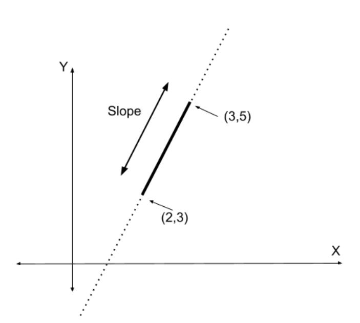
Now, say you’re given two points on this line, let’s say they are at x=2, y = 3 and at x=3, y=5, how would we write code that figures out the values of W and B that describe the line joining these two points?
Let’s start with W, which we call the weight, but in geometry, it’s also called the slope (sometimes gradient). See Figure 1-2.
Figure 1-2. Visualizing a Line Segment withSlope
Calculating it is easy:
W = (y2-y1)/(x2-x1)
So if we fill in, we can see that the slope is:
W = (5-3)/(3-2) = (2)/(1) = 2
Or, in code, in this case using Python:
def get slope(p1, p2):
W = (p2.y - p1.y) / (p2.x - p1.x)
return W
This function sort of works. It’s naive because it ignores a divide by zero when the two x values are the same, but let’s just go with it for now.
Ok, so we’ve now figured out the W value. In order to get a function for the line, we also need to figure out the B. Back to high school geometry, we can use one of our points as an example.
So, if
y = Wx + B
We can also say:
B = y - Wx
And we know that when x=2, y=3, and W=2 we can back fill this function:
B = 3 - (2*2)
Which leads us to derive that B is -1.
Again, in code, we would write:
def get bias(p1, W):
B = p1.y - (W * p1.x)
return B
So, now, to determine any point on the line, given an x, we can easily say:
def get y(x, W, B):
y = (W*x) + B
return y
Or, for the complete listing:
def get slope(p1, p2):
W = (p2.y - p1.y) / (p2.x - p1.x)
return W
def get bias(p1, W):
B = p1.y - (W * p1.x)
return B
def get y(x, W, B):
y = W*x + B
p1 = Point(2, 3)
p2 = Point(3, 5)
W = get slope(p1, p2)
B = get bias(p1, W)
# Now you can get any y for any x by saying:
x = 10
y = get y(x, W, B)
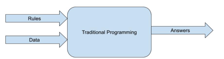
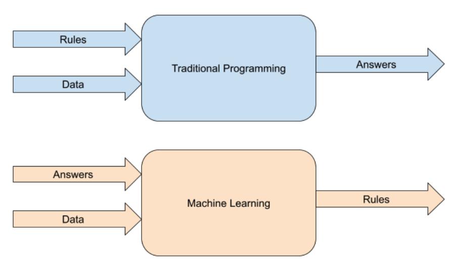
From these, we could see that when X is 10, Y will be 19..You’ve just gone through a typical programming task. You had a problem to solve, and you could solve the problem by figuring out the rulesand then expressing them in code. There was a ruleto calculate W when given 2 points, and you created that code. You could then, once you’ve figured out W, derive another rule when using W and a single point to figure out B. Then, once you had W and B, you could write yet another rule to calculate y in terms of W, B and a given x. That’s traditional programming, which is now often referred to as rulesbased programming. I like to summarize this with the diagram in Figure 1-3.
Figure 1-3. TraditionalProgramming.
At its highest level, Traditional Programming involves creating Rules that act on Dataand which give us Answers. In the above scenario, we had data -- 2 points on a line. We then figured out the rules that would act on this data to figure out the equation of that line. Then, given those rules, we could get answers for new items of data, so that we could, for example, plot that line.
The core job of the programmer in this scenario is to figureoutthe rules. That’s the value you bring to any problem -- breaking it down into the rules that define it, and then expressing those rules in terms that a computer can understand using a coding language.
But you may not always be able to express those rules easily. Consider the scenario from earlier when we wanted to differentiate between a tee-shirt and a boot. One could not always figure out the rules to determine between them, and then express those rules in code. Here’s where Machine Learning can help, but before we go into it for a computer vision task like that, let’s consider how Machine Learning might be used to figure out the equation of a line like we had done above.
How can a Machine Learn?
Given the above scenario, where you as a programmer figured out the rules that make up a line, and the computer implemented them, let’s now see how a Machine Learning approach would be different. Let’s start by understanding how Machine Learning code is structured. While this is very much a ‘hello world’ problem, the overall structure of the code is very similar to what you’d see even in far more complex ones.
I like to draw a high level architecture of using Machine Learning to solve a problem like this. Remember, in this case, we’ll have x and y values, so we want to figure out the W and B so that we have a line equation, and once we have that equation, we can then get new y values given x ones.
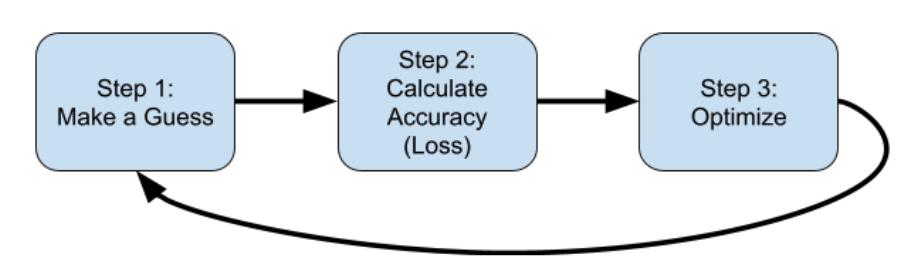
Step 1. Guess the answer.
Yes, you read that right. To begin with, we have no idea what the answer might be, so a guess is as good as any other answer. In real terms this means we’ll pick a random value for W and B. We’ll loop back to this step with more intelligence a little later, so subsequent values won’t be random, but we’ll start purely randomly. So, for example, let’s assume that our first ‘guess’ is that W = 10, and B = 5.
Step 2. Measure the accuracy of our guess.
Now that we have values for W and B, we can use these against our known data to see just how good, or how bad, those guesses are. So, we can use y=10x+5 to figure out a y for each of our x values, compare that y against the ‘correct’ value, and use that to derive how good or how bad our guess is. Obviously, for this situation our guess is really bad because our numbers would be way off. We’ll go into detail on that shortly, but for now, we realize that our guess is
really bad, andwe have a measure of how bad. This is often called the loss.
Step 3. Optimize our guess.
Now that we have a guess, and we have intelligence about the results of that guess (or the loss), we have information that can help us create a new and better guess. This process is called optimization.If you’ve looked at any AI coding or training in the past and it was heavy on mathematics, it’s likely you were looking at optimization. Here’s where fancy calculus, in a process called GradientDescentcan be used to help make a better guess. Optimization techniques like this figure out ways to make small adjustments to your parameters that drive towards minimal error. I’m not going to go into detail on that here, and while it’s a useful skill to understand how optimization works, the truth is that frameworks like TensorFlow implement them for you so you can just go ahead and use them. In time, it’s worth digging into them for more sophisticated models, allowing you to tweak their learning behavior. But for now, you’re safe just using a built-in optimizer. Once you’ve done this, you simply go to step 1.
Repeating this process, by definition, helps us over time, and many loops to figure out the parameters W and B.
And that’s why this process is called MachineLearning. Over time, by making guesses, figuring out how good or how bad that guess might be, optimizing the next guess based on that intel, and then repeating, the computer will ‘learn’ the parameters for W and B (or indeed anything else), and from there, it will figureoutthe rules that make up our line.
Visually this might look like Figure 1-4.
Figure 1-4. The Machine Learning Algorithm.
Implementing Machine Learning in Code
That’s a lot of description, and a lot of theory. Let’s now take a look at what this would look like in code, so you can see it running for yourself. A lot of this code may look alien to you at first, but you’ll get the hang of it over time. I like to call this the ‘Hello World’ of Machine Learning, as you use a very basic neural network (which I’ll explain a little later), to ‘learn’ the parameters W and B for a line, when given a few points on the line.
Here’s the code (a full notebook with this code sample can be found in the github for this book):
model = Sequential(Dense(units=1, input shape=[1]))
This is written using the TensorFlow Keras APIs. Keras is an open source framework designed to make definition and training of models easier with a high level API. It became tightly integrated into TensorFlow in 2019 with the release of TensorFlow 2.0
Let’s explore this line by line. First of all is the concept of a model. When creating code that learns details about data, we often use the term model to define the resultant object. A model, in this case, is roughly analogous to the get_y() function from the coded example earlier. What’s different here is that the model doesn’t needto be given the W and the B. It will figure them out for itself based on the given data, so you can just ask it for a y and give it an x, and it will give you it’s answer. So our first line of code looks like this -- it’s defining the model.
model = Sequential(Dense(units=1, input shape=[1]))
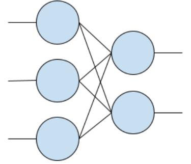
But what’s the rest of the code? Well, let’s start with the word ‘Dense’ which you can see within the first set of parentheses. You’ve probably seen pictures of neural networks that look a little like Figure 1-5.
Figure 1-5. Basic NeuralNetwork
You might notice that in Figure 1-5, each circle (or neuron) on the left is connected to each neuron on the right. Every neuron is connected to every other neuron in a dense manner. Hence the name ‘Dense’. Also, there are three stacked neurons on the left, and two stacked neurons on the right, and these form very distinct ‘layers’ of neurons in sequence, where the first ‘layer’ has 3 neurons, and the second has 2 neurons.
So let’s go back to the code.
model = Sequential(Dense(units=1, input shape=[1]))
This code is saying that we want a sequence of layers (‘Sequential’), and within the parentheses, we will define those sequences of layers. The first in the sequence will be a ‘Dense’, indicating a neural network like that in Figure 1-5. There’s no other layers defined, so our sequential just has 1 layer. This layer has only 1 unit indicated by the units=1 parameter, and the input shape to that unit is just a single value.
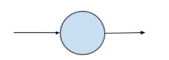
So our neural network will look like Figure 1-6:
Figure 1-6. Simplest Possible NeuralNetwork.
This is why I like to call this the ‘Hello World’ of Neural Networks. It has 1 layer, and that layer has 1 neuron. That’s it. So, with that line of code we’ve now defined our model architecture. Let’s move on to the next line:
Here we are specifying builtinfunctions to use to calculate the loss (remember step 2, where we wanted to see how good or how bad our guess was), and the optimizer (step 3, where we generate a new guess), so that we can improve on the parameters within the neuron for W and B.
In this case ‘sgd’ stands for ‘Stochastic Gradient Descent’, which is beyond the scope of this book, but in summary it uses calculus alongside the mean squared error loss to figure out how to minimize loss, and once loss is minimized we should have parameters which are accurate.
Next, let’s define our data. 2 points may not be enough, so I expanded it to six points for this example:
The ‘np’ stands for ‘numpy’, a Python library commonly used in data science and machine learning and which makes handling of data very straightforward. You can learn more about numpy at https://numpy.org/.
We’ll create an array of x values, and their corresponding y values, so that given x = -1, y will be -3, when x is 0, y is -1 and so on. A
quick inspection shows that you can see the relationship of y=2x-1 holds for these values.
Next let’s do the loop that we had spoken about earlier -- make a guess, measure how good or how bad that loss is, optimize for a new guess and repeat. In TensorFlow parlance this is often called ‘fitting’, namely we have xs and ys, and we want to fit the xs to the ys, or, in other words, figure out the rule that gives us the correct y or a given x using the examples we have. The epochs=500 parameter simply indicates that we’ll do the loop 500 times:
model.fit(xs, ys, epochs=500)
When you run code like this (you’ll see how to do this later in this chapter if you aren’t already familiar with it), you’ll see output like the following:
Note the ‘loss’ value. The unit doesn’t really matter, but what does is that it is getting smaller. Remember the lower the loss, the better your model will perform, and the closer its answers will be to what you expect. So the first guess was measured to have a loss of 32.4543, but by the 5th guess this was reduced to 13.3362.
If we then look at the last 5 epochs of our 500, and explore the loss:
This is indicating that the values of W and B that the neuron has figured out are only off by a tiny amount. It’s not zero, so we shouldn’t expect the exact correct answer. For example, if we give it x=10, like this:
print(model.predict([10.0]))
The answer won’t be 19, but a value verycloseto 19, and it’s usually about 18.98. Why? Well there’s two main reasons. The first is that neural networks like this deal with probabilities, not certainties, so that the W and B that it figured out are ones that are highly probableto be correct, but may not be 100% accurate. The second reason is that we only gave 6 points to the neural network. While those 6 points arelinear, that’s not proof that every other point that we could possibly predict is necessarily on that line. The data could skew away from that line...there’s a very low probability that this is the case, but it’s non-zero. We didn’t tellthe computer that this was a line, we just asked it to figure out the rule that matched the xs to the ys, and what it came up with looks like a line, but isn’t guaranteed to be one.
This is something to watch out for when dealing with neural networks and machine learning -- you will be dealing with probabilities like this!
There’s also the hint in the method name on our model -- notice that we didn’t ask it to calculatethe y for x=10.0, but instead to predict it. In this case a prediction (often called an inference) is reflective of the fact that the model will tryto figure out what the value will be based on what it knows, but it may not always be correct.
Comparing Machine Learning with Traditional Programming
Referring back to Figure 1-3 for Traditional programming, let’s now update it to show the difference between Machine Learning and Traditional Programming given what you just saw. Earlier we described Traditional Programming as you figure out the rules for a given scenario, express them in code, have that code act on data, and you’ll get answers out. Machine Learning is very similar, except that some of the process is reversed. See Figure 1-7.
Figure 1-7. From TraditionalProgramming to Machine Learning.
As you can see the key difference here is that with Machine Learning youdonotfigureouttherules!Instead you provide it answers and data, and the Machine will figure out the rules for you. In the above example, we gave it the correct y values (aka the answers) for some given x values (aka the data), and the computer figured out the rules that fit the x to the y. We didn’t do any geometry, slope calculation, interception or anything like that. The machine figured out the patterns that matched the xs to the ys.
That’s the coreand importantdifference between Machine Learning and Traditional Programming, and it’s the cause of all of the excitement around Machine Learning because it opens up whole new
scenarios of application. One example of this is computer vision -- as we discussed earlier, trying to write the rulesto figure out the difference between a tee shirt and a boot would be much too difficult to do. But having a computer figure out how one matches to another makes this scenario possible, and from there scenarios that are more important -- such as interpreting X-rays or other medical scans, detecting atmospheric pollution, and a whole lot more becomes possible. Indeed, research has shown that in many cases using these types of algorithms along with adequate data has led to computers being as good as, and sometimes better than humans at particular tasks. For a bit of fun, check out this blog post about diabetic retinopathy -- where researchers at Google trained a neural network on pre-diagnosed images of retinas, and had the computer figure out what determines each diagnosis. The computer, over time, became as good as the best of the best at being able to diagnose the different types of diabetic retinopathy!
Here you saw a very simple example of how you transition from rules-based programming to ML to solve a problem. But it’s not much use solving a problem if you can’t get it into your user’s hands, and with ML models on mobile devices running Android or iOS, you’ll do exactly that!
It’s a complicated and varied landscape, and in this book we’ll aim to make that easier for you, through a number of different methods. For example, you might have a turnkey solution available to you, where an existingmodel will solve the problem for you, and you just want to learn how to do that. We’ll cover that for scenarios like Face Detection, where a model will detect faces in pictures for you, and you want to integrate that into your app.
Additionally, there are many scenarios where you don’t need to build a model from scratch, figuring out the architecture, and going through long and laborious training. A scenario called Transfer Learningcan often be used, and this is where you are able to take parts of pre-existing models and repurpose them for your own. For example, Big Tech companies, and researchers at top Universities have access to data and computer power that you may not, and they have used that to build models. They’ve shared these models with the world so they can be re-used and repurposed. You’ll explore that a lot in this book, starting in Chapter 2.
Of course, you may also have a scenario where you need to build your own model from scratch. This can be done with TensorFlow, but we’ll only touch on that lightly here, instead focussing on mobile scenarios. The partner book to this one, called AIandMachine LearningforCodersfocuses heavily on that scenario, teaching you from first principles how models for various scenarios can be built from the ground up.
Summary
In this Chapter you got an introduction to what Artificial Intelligence and Machine Learning are. Hopefully it helped cut through the hype so you can see, from a programmer’s perspective, what it really is all about, and from there you could identify the scenarios that it can be extraordinarily useful and powerful for implementing. You saw, in detail, how Machine Learning works, and the overall ‘loop’ that a computer uses to learn how to fit values to each other, matching patterns, and ‘learning’ the rules that put them together. From there, the computer could act somewhat intelligently, lending us the term ‘Artificial’ intelligence. You learned about the terminology of being an Machine Learning or Artificial Intelligence programmer including models, predictions, loss, optimization, inference and more. From Chapter 3 onwards you’ll be using examples of these to implement
machine learned models into mobile apps. But first, let’s explore building some more models of our own to see how it all works, so in Chapter 2 you’ll look into building some more sophisticated ones for Computer Vision!
Chapter 2. Introduction to Computer Vision
A NOTE FOR EARLY RELEASE READERS
With Early Release ebooks, you get books in their earliest form— the author’s raw and unedited content as they write—so you can take advantage of these technologies long before the official release of these titles.
This will be the 2nd chapter of the final book. The GitHub repo is https://github.com/lmoroney/odmlbook.
If you have comments about how we might improve the content and/or examples in this book, or if you notice missing material within this chapter, please reach out to the editor at jleonard@oreilly.com.
While this book isn’t designed to teach you all of the fundamentals of architecting and training Machine Learned models, I do want to cover some basic scenarios so that the book can still work as a standalone. If you want to learn more about the model creation process with TensorFlow, I recommend my book AIandMachine LearningforCoderspublished by O’Reilly, and if you want to go deeper than that, Aurelien Geron’s excellent book HandsonMachine LearningwithScikit-Learn,KerasandTensorFlowis a must!
In this chapter, we’ll go beyond the very fundamental model you created in Chapter 1, and look at two more sophisticated ones, where you will deal with computer vision -- namely how computers can ‘see’ objects. Similar to the terms ‘Artificial Intelligence’ and ‘Machine Learning’, the phrase ‘Computer Vision’ and ‘seeing’ might
lead one to misunderstand what is fundamentally going on in the model.
Computer Vision is a huge field, and for the purposes of this book and this chapter, we’ll focus narrowly on a couple of core scenarios- where we will use technology to parse the contents of images, either labelling the primary content of an image, or finding items within an image.
It’s not really about ‘vision’ or ‘seeing’, but more having a structured algorithm that allows a computer to parse the pixels of an image. It doesn’t ‘understand’ the image any more than it understands the meaning of a sentence when it parses the words into individual strings!
If we were to try to do that task using the traditional rules based approach, we would end up with many lines of code for even the simplest images. Machine Learning is a key player here, and as you’ll see in this chapter, using the same pattern of code that we had had in chapter 1, but getting a little deeper, we can create models that can parse the contents of images...with just a few lines of code. So let’s get started.
Using Neurons for Vision
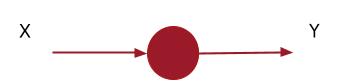
In the example you coded in Chapter 1, you saw how a neural network could ‘fit’ itself to the desired parameters for a linear equation when given some examples of the points on a line in that equation. Represented visually, our neural network could look like Figure 2-1.
Figure 2-1. Fitting an Xto a Ywitha neuralnetwork
This was the simplest possible neural network, where there was only 1 layer, and that layer had only 1 neuron.
NOTE
In fact I cheated a little bit when creating that example because neurons in a dense layer are fundamentally linear in nature as they learn a weight and a bias, so a single one is enough for a linear equation!
But when we coded this, recall that we created a Sequential, and that Sequential contained a Dense, like this: model = Sequential(Dense(units=1))
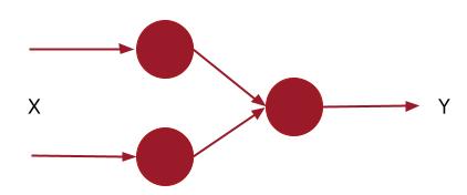
We can use the same pattern of code if we wanted to have more layers, so, for example if we wanted to represent a neural network like that in Figure 2-2, it would be quite easy to do.
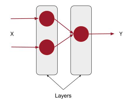
First, let’s consider the elements within the diagram of Figure 2-2. Each vertical arrangement of neurons should be considered a Layer. So, Figure 2-3 shows us the layers within this model.
Figure 2-2. ASlightly more advancedNeuralNetwork
Figure 2-3. Showing the layers within the neuralnetwork.
So, to code these, we simply list them within the Sequential definition, updating our code to look like this:
model = Sequential( [Dense(units=2), Dense(units=1)])
We simply define our layers as a comma separated list of definitions, and put that within the Sequential, so as you can see here, there’s a Dense with 2 units, followed by a Dense with 1 unit, and we get the architecture as shown in Figure 2-3.
But in each of these cases our outputlayer is just a single value. There’s 1 neuron at the output, and given that that neuron can only learn a weight and a bias, it’s not very useful for understanding the contents of an image, because even the simplest image has too much content to be represented by just a single value.
So what if we have multipleneurons on the output?
So, for example if we define a model that looks like Figure 2-4.