4. Deriving the De Broglie Relationship
We can derive the De Broglie relationship from the Amplitude of a string.
Using the following relationship and inputting the frequency,
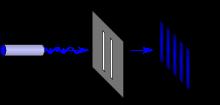
We have, Where Distance of the closed string = Louis De Broglie described the amplitude of matter particles and their wave-like nature.
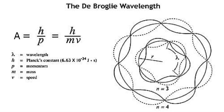
Fig. 4: De Broglie’s theorem describes the amplitude of matter particles.
8
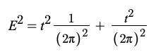
A = c 2π f hf = mc 2 f = mc 2 h A = hc 2π mc 2 = h 2π mc = h 2π m( λ / t ) = h m( v ) 2πλ
5. Theoretical explanation that gravity is the Grand Unified Force. Our experimental proof will follow after this chapter.
The String Theory Work Function is the most powerful mathematical derivation of string theory. It is fairly simple at first glance, but it’s the reason for all universal dynamics in the universe, so the derivation should not be underestimated.
x = A i Sin( wt )
dx
dt = A i w i Cos( wt )
A = c 2π f
d 2 y
dx 2 = A i w2 i sin( wt )
d 2 y
dx 2 = c 2π f i ( 2π f )2 i sin( wt ) = c i ( 2π f ) i sin( wt )
Where the negative represents the inward acceleration of the Grand Unified Force. This will be proved theoretically and experimentally in the next section of this paper.
a = −2π fc
The string theory work function is (mass times acceleration times distance):
m i a i x = m i ( 2π fc ) i x
if we substitute for the frequency in the acceleration term:
E = hf = mc 2
f = mc 2 h a = 2π fc
Another way to express the acceleration:
a = 2π mc 3 h
9
Using the string theory work function we can show that its equal to the rest mass energy as proposed by Albert Einstein.
Substituting for x and the acceleration. We find:
10
a = 2π fc x = c 2π f max = m i ( c i 2π f ) i c 2π f = mc 2
6. Using experimental data of the Photoelectric Effect to prove the validity of the String Theory’s Work Function with less than 1 percent error.
Einstein developed an experiment to determine the energy in light. When monochromatic light is beamed at an emitter plate he noticed that there was a current produced. If you apply a voltage in the opposite direction of the current we can cancel out the current.
With the experimental evidence that I am citing the current produced by the light is 0.071A in the circuit and the cathode is made out of sodium metal
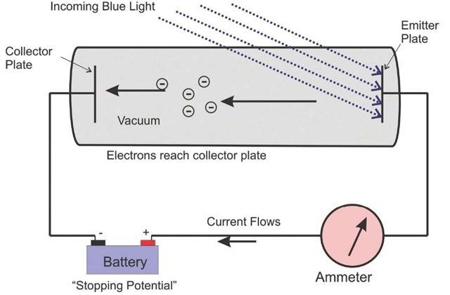
Fig 5. The Photoelectric effect. Light is beamed at the cathode made out of Sodium. A stopping potential is applied to stop the current.
We can derive an expression to explain the photoelectric effect using the string theory work function and with consideration in solid state physics.
As we derived we notice that light pushes things backward
We can begin to derive the equation that describes the photoelectric effect, by first deriving all the terms of the equation.
Recall that the energy of light is expressed as follows:
hf
11
WStringTheoryWorkFunction
stopping potential
a = 2π fc
= Elight E
+ E Fermi Energy Elight =
The energy required to stop the current from flowing is called the stopping potential and its expressed as follows
E stopping potential = qV
The total amount of work that the light performs to excite the electron from its ground state to its free state, with kinetic energy, is given by the string theory Work Function. We can re-express the equation to eliminate the mass, of light, from the expression.
mc 2 = fh m = fh
The next term in our equation that we will be using was derived by Enrico Fermi. However, I found a mistake in his equation. And it’s important that we derive the mistake to explain the correction before we move on to explaining the experimental data.
The following is unit analysis:
E = mv 2
E = ML2T 2
ET 2 = ML2
ET = ML2T 1
ET = PL
h ⋅ f ⋅ T = PL
h = PL
The important part of this is that the solution derives planck constant. Not the Reduced planck constant, because that adds an extra 2pi that does not correspond to the unit analysis that we just described. This is an important distinction in the derivation.
12
c
x 2
ht x 2 m( 2π fc ) x = ht x 2 2π fcx ( ) = 2π hc x = 2π hc λ
π hc λ
c 2 = fh
2 = fht 2
=
WStringTheoryWorkFunction = 2
For the Fermi Energy derivation, I took a look at the Introduction to Solid State Physics by Charles Kittel [4]
The following is the Fermi Energy with a correction.
Recall that:
E = p 2 2 m = 1 2 mv 2
h = PL
2 = P
We remove the reduced planck constant to correct the derivation.
Thus, the Fermi energy is as follows.
13
pψ k
fermi
p 2 L2 2 m 2π ( )2 k f 2 = ! 2 2π ( )2 2 m k f 2
⎝ ⎜ ⎞ ⎠ ⎟ 2 / 3
h
2 L2 L = 2π L2 = 2π ( )2
r ( ) = E
=
E fermi = h 2 2 m 3π 2 N V ⎛
Now we can derive the equation that will describe the Photoelectric Effect as Follows.
On the left, we have the string theory work function, which represents all the Work light does on the electrons in the photoelectric effect.
The first term on the right side represents the kinetic energy the light will gain after it satisfied the potential energy required to reach the unbound state. This produces the kinetic energy associated with the current.
The next term is the stopping potential. This is the experimental voltage used to stop the flow of current. At the instance where the stopping potential stops the current, this corresponds to the maxed-out Fermi Energy.
And the last term, the Fermi Energy, is the Potential energy. Its the energy difference between the highest and lowest occupied particle state occupied by the electrons.
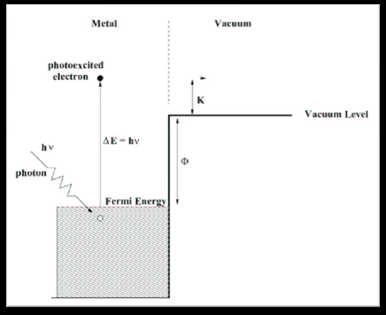
Fig. 6: This schematic shows a ray of light exciting the electron in a Sodium atom. The light does work on the electron to fill the Fermi Energy potential energy. This is the energy associated with the energy required to go from the ground state to the highest occupied state. If there is any energy left the electron gains Kinetic Energy E=hf.
14
2π hc λ o = hf qV + h 2 2 m 3π 2 N V ⎛ ⎝ ⎜ ⎞ ⎠ ⎟ 2 / 3
The next thing we need to do is to find all the experimental values for the Number of electrons divided by the volume they occupy, the number density of free electrons.
Our experimental setup is titled “Photoelectric Effect Prelab” by Dr. Christine P Cheney of the Department of Physics and Astronomy from the University of Tennessee. [5]
The first thing we want to do is calculate the Number Density of free electrons The reason we can figure this number out experimentally is that when we stop the voltage we cancel out the kinetic energy produced by the incident light and we fill the Fermi Energy level to its highest level
f = 7.49481145 ⋅ 1014 hz
λ = 400 ⋅ 10 9 m
q = 1.602176634 ⋅ 10 19 Coulomb
h = 6.62607004 10 34 m 2 kg / s
Vstopping = 0.72Volts
c = 299, 792, 458
m e = 9.1093837015 ⋅ 10 31 kg
N V = 2π hc
Plugging in all of these variables gives us the electron density.
N V = 1.29416 ⋅ 10 27 electrons / m 3
15
2π hc λ o hf + qV = h 2 2 m 3π 2 N V ⎛ ⎝ ⎜ ⎞ ⎠ ⎟ 2 / 3
π hc λ
⎛ ⎝ ⎜ ⎞ ⎠ ⎟ 2 m h 2 ⎛ ⎝ ⎜ ⎞ ⎠ ⎟ = 3π 2 N V ⎛ ⎝ ⎜ ⎞ ⎠ ⎟ 2 / 3 2π hc λ o hf + qV ⎛ ⎝ ⎜ ⎞ ⎠ ⎟ 2 m h 2 ⎛ ⎝ ⎜ ⎞ ⎠ ⎟ ⎛ ⎝ ⎜ ⎞ ⎠ ⎟ 3/ 2 = 3π 2 N V N
2π hc λ o hf + qV ⎛ ⎝ ⎜ ⎞ ⎠ ⎟ 2 m h 2 ⎛ ⎝ ⎜ ⎞ ⎠ ⎟ ⎛ ⎝ ⎜ ⎞ ⎠ ⎟ 3/ 2 1 3π 2 ⎛ ⎝ ⎜ ⎞ ⎠ ⎟
2
o hf + qV
V =
λ
⎛ ⎝ ⎜ ⎞ ⎠ ⎟ 2 m h 2 ⎛ ⎝ ⎜ ⎞ ⎠ ⎟ ⎛ ⎝ ⎜ ⎞ ⎠ ⎟ 3/ 2 1 3π 2 ⎛ ⎝ ⎜ ⎞ ⎠ ⎟
o hf + qV
To derive what Einstein called the Work Function theoretically we need to calculate the total work that light does on the electrons and subtract the Fermi Energy. The work function is the energy associated with the protons electrostatic attraction on the electrons.
If we solve for the work function using the calculated Number Density and the light at 400nm. We get a theoretical value for the Work Function of 2.38 Ev. The experimental value for the work function is 2.36 eV [6]. Since we know the cathode in the experiment is made out of sodium - the work function matches. Thus, we proved the String Theory Work Function to be correct with a 0.84% error.
ϕExperimental = 2.36 eV
= 0.84%
If we increase the frequency and stop the stopping potential voltage, the equation simplifies to Einstein’s Photoelectric effect equation.
We can verify the stoping voltage as follows
Ek = hf ϕ
If we increase the frequency and stop the stopping potential voltage the electrons will gain kinetic energy [7]
Ek = hf ϕ hf = (6.62607004 10 34 m 2 kg / s ) 299, 792, 458 m / s 400 10 9
= 4.96611456 10 19 J
ϕ = 2.38ev = 2.38eV ( ) i 1.602176634 ⋅ 10 19 C ( ) = 3.813180389 ⋅ 10 19 Joules
E K = 4.96611456 ⋅ 10 19 J 3.813180389 ⋅ 10 19 Joules = 1.152934171 ⋅ 10 19 Joules
16
ϕ = 2π hc λ h 2 2 m 3π 2 N V ⎛ ⎝ ⎜ ⎞ ⎠ ⎟ 2 / 3
Percent
ϕtheoretical = 2.38eV
Error = ϕtheoretical ϕExperimental ϕtheoretical = 2.38eV 2.36 eV 2.38eV x100%
⎛ ⎝ ⎜ ⎞ ⎠ ⎟
m
Using the current equations we can derive the stopping voltage to be accurate. And thus we conclude that the string theory work function does yield the right work function. And the experimental setup has the correct energy for the stopping potential.
The power is given by the current times the voltage.
P = iV
E t = q t ⋅ V
E = qV
V = E q
V = E q = 1.152934171 ⋅ 10 19 Joules
1.602176634 10 19 C
Ek = hf ϕ qV = 0
= 0.72V
17
⎛ ⎝ ⎜ ⎞ ⎠ ⎟
7. Deriving the Planck Length, Planck Time, Planck Mass Derivation using the String Theory Work Function!
In this section, we derive the work established by Max Planck. Previously Max Planck derived the Planck Length, Planck Time, and Planck mass using dimensional analysis, but in this paper, we will derive it with the string theory work function.
Deriving the Planck Length:
G = 6.67408 i 10 11 m 3 / kg s 2
h = 6.62607004 i 10 34 m 2 kg / s
c = 299792458 m / s
If we equate the gravitational energy to the string theory work function we can independently derive the Planck length. Which corresponds to the smallest string length possible for a single string
GMm r = m2π fcx
x = r x 2 = GM fc i 2 i π
M = hf c 2
PlanckLength = Gh 2π c 3 = 1.616228373 i 10 35 m
18
Deriving Planck Time:
Planck Length divided by the speed of light gives us Planck time. Which corresponds to the time it takes to travel the smallest strings length at the speed of light
PlanckTime = Gh 2
= 5.391157549 i 10 44 s
Deriving the Planck Mass:
GMm r = m2π fcx
x = r
GMm = m2π fcx 2
GM = 2π fcx 2
If x is equal to lambda:
xf = λ f = c
GM = 2π c 2 x
x = h Mc
GM = 2π c 2 h
Mc
M 2 = 2π ch
G
M = 2π ch
G = 1.367516555 i 10 7 kg
The planck mass is the maximum mass a string can have when it has its maximum carrying capacity with 299,792,458 electric fields. It is important to note that the derivation of this is found at the conclusion of the paper.
19
π
πc5
c 3 c = Gh 2
The following is the derivation that the highest frequency and mass a single string can have is as follows:
c = 299, 792, 458 m / s
m planck = 1.367516555 10 7 kg
h = 6.62607004 i 10 34 m 2 kg / s
m planck = 1.367516555 10 7 kg
t planck time = 5.391157549 10 44 s
hf = m planck ⋅ c 2
The maxiumum frequency a string can have on its own is:
f = 1 / t planck time = 1 5.391157549 10 44 s = 1.854889216 i 10 43 Hz
hf = 1.854889216 i 10 43 Hz ( ) 6.62607004 i 10 34 m 2 kg / s ( ) = 1.229062586 i 1010 J
m planck c 2 = (1.367516555 10 7 kg )( 299792458) 2 = 1.229062586 1010 J
hf = m planck ⋅ c 2
Thus if a string is traveling at the speed of light it carries a Planck Mass. However, at the end of this paper, we will prove that if light slows down, the number of electric fields the individual string carries diminishes.
20
The following is the derivation of the Planck Energy:
The planck energy is the maximum work that can be done to a string to max out the carrying capacity of the string.
2π fc = GM r 2
x = c 2π f
2π fc = GM i 4π 2 f 2 c 2
2πc3
GM ( 4π 2 ) = f
f = c 3 GM 2π
mc 2 = hf
m = hf c 2
f = c5 G ( hf )2π
f 2 = c5 Gh2π
f = c5 Gh2π
E planck = hf = h c5 Gh2π ⎛ ⎝ ⎜ ⎜ ⎞ ⎠ ⎟ ⎟ = c5h G 2π
If the signal travels slower than the speed of light.
f = v 5/ 2 1 Gh2π ⎛ ⎝ ⎜ ⎞
21
⎠ ⎟
1/ 2
The maximum work on a single string is:
h = 6.62607004 i 10 34 m 2 kg / s
c = 299, 792, 458m / s
G = 6.67408 i 10 11 m 3 / kg ⋅ s 2
W = hf = c 5 h 2πG
⎝ ⎜ ⎞ ⎠ ⎟ 1/ 2 = 1.956113860 ⋅ 109 Joules
At this energy, the energy of a single string is at its theoretical maximum. Coincidentally, this is about the energy observed in lightning bolt due to the string carrying capacity. Due to the constructive nature of strings, energies can be larger if more than one string is present. Otherwise, higher energies found in nature wouldn’t be possible.
We can calculate the maximum amplitude of the strings to be as follows:
Amplitude = c 2π f = ch 2π fh = 299, 792, 458 m / s ( ) (6.62607004 ⋅ 10 34 m 2 kg / s ) 2π (1.956113860 ⋅ 109 J ) = 1.616228373 i 10 35 m
This amplitude is the same value found in the planck length calculation, because, this is the smallest size a string could theoretically have.
22
⎛
8. Center Of Mass Action in Hurricanes
Gravity is the central acting mechanism behind hurricane formation. The center of mass provides the energy required to form the centripetal acceleration found in hurricanes. While gravity is responsible for wind velocity and mass accumulation, the category of the hurricane is not dependent on mass, the strength of the winds is in large part due to the accumulation of water vapor and thermodynamic effects.
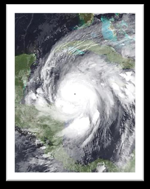
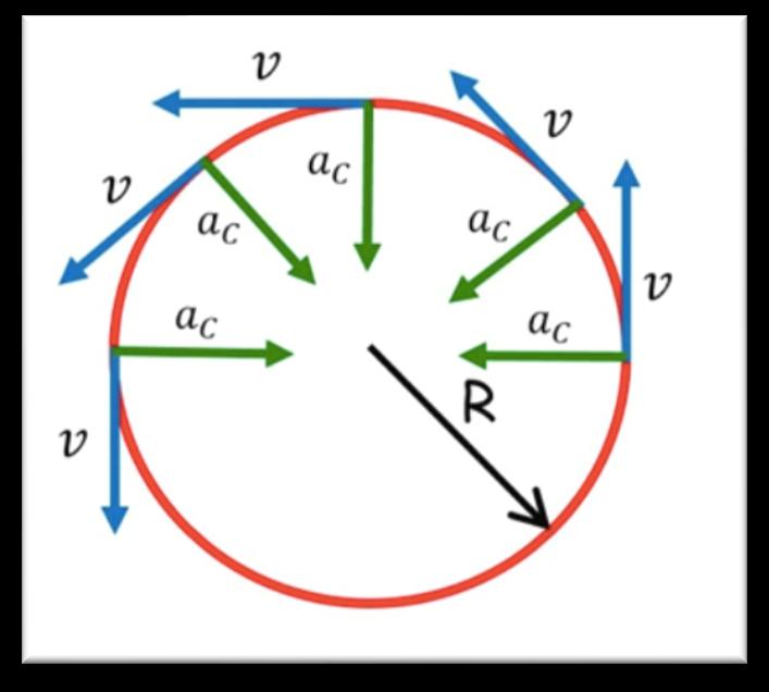
Fig. 7: The centripetal acceleration of hurricanes is due to the String Theory Work Function.
A hurricane is very similar to a black hole as we will develop in this paper consequently. All the mass of the hurricane produced by the water vapor concentrates the gravitational signal inward towards the center of the eye. And it’s very similar to a Schwarzschild radius. The particles at the center don’t have much kinetic energy because they are in a large gravitational well and it takes enough energy to break free at the eye wall.
23
WGravitational Well = F d = GMm r 2 d = GMm r 2 r WGravitational Well 1 2 mv 2 = 0 1 2 m atoms v 2 = GM Hurricane m atoms reyewall
The escape speed of air in Hurricanes occurs at the eye-wall. It’s similar to a rocket launching from the earth. If it doesn’t have enough escape speed, the rocket wouldn’t be able to escape the gravitational well. In this case, it’s air molecules escaping the hurricane’s gravitational field. It is important to note that the mechanism for hurricanes was never completely understood until now.
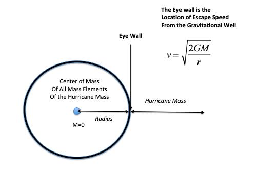
Fig. 8: The air has enough centripetal acceleration in the eye wall to break free from the gravitational well. This is why the highest speed of wind of the hurricane is found in the eye wall.
Deriving the Mass of Hurricanes
Particles in the eye wall have centripetal acceleration and escape speed. If we know the radius of the eye wall and the speed of the wind at the eye wall we can calculate the mass of the hurricane.
eyewall
Radar data can be used to study hurricane dynamics with greater accuracy. However, I tabulated a theoretical calculation of all the hurricane velocities using the lower and high limits of the Saffir-Simpson Hurricane Wind Scale speed. And I tabulated all of the theoretical yields with eye-walls from 1 – 20 miles radius.
I would like to denote that the scale is very accurate. If you notice in the Table 1, the range of Average mass of water vapor in the hurricane, per hurricane category, correlates with the wind linearly.
24
M
Hurricane = veyewall 2 i r
2G
Saffir-Simpson Hurricane Wind Scale
Eye Wall Radius 1-20 miles
Category 3: 178-208 km/h
Category 4: 209-251 km/h
Table 1: The Saffir-Simpson Hurricane Wind Scale correlates linearly with the average increase in the mass of the hurricane.
The following are all my theoretical calculations for all categories of hurricanes ranging from 1 mile to 20 mile radius of eye walls. I choose this range because hurricane Wilma has the smallest eye wall with a 2 mile diameter and most hurricanes fall within 40 mile diameters.
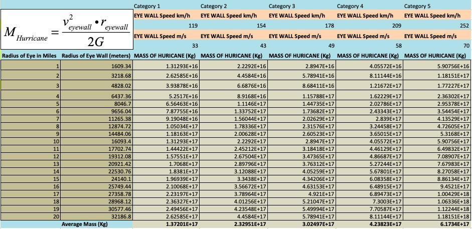
Table 2: This table shows the theoretical mass generated by each hurricane category at the lowest wind speed for each hurricane Category given by the SaffirSimpson Hurricane Scale.
25
Wind Speed Average Mass in Kg
1.37E16
Category 1: 119-153 km/h
- 2.34E17
Category 2: 154-177 km/h 2.33E17 - 3.02E17
3.02E17 - 4.24E17
4.24E17
252 km/h
higher 6.17E17
8.47E17++
- 6.17E17 Category 5:
or
-
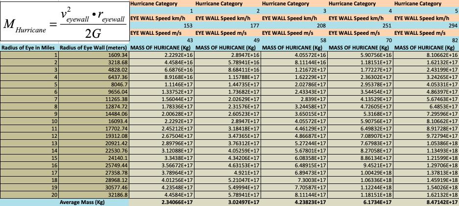
Table 3: This table shows the theoretical mass generated by each hurricane category at the highest wind speed for each hurricane Category given by the SaffirSimpson Hurricane Scale.
26
While the hurricane averages are useful in validating the usefulness of the Saffir –Simpson Hurricane Wind scale. It’s important to find the lowest and highest mass in hurricanes to see the range of mass in each category of hurricane. The following table describes this data (see Table 4)
Category 1 Lowest to Highest Mass in Kg
1.31E16 -4.46E17
Category 2 Lowest to Highest Mass in Kg
2.23E16-5.79E17
Category 3 Lowest to Highest Mass in Kg
2.89E16-8.11E17
Category 4 Lowest to Highest Mass in Kg
4.055E16-1.18E18
Category 5 Lowest to Highest Mass in Kg
5.91E16-1.62E18++
Table 4: This table shows the range of mass in each Hurricane category based on the Saffir-Simpson Wind Scale.
Now that we know the theoretical range of mass that each category of the hurricane has, we can analyze the mass produced by hurricanes (with historical records from data from the National Hurricane Center).
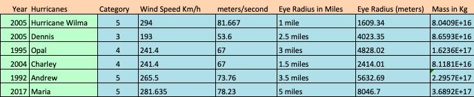
Table 5: The data found from the National Hurricane Center shows that the masses of the hurricanes lie well within the range of expected mass [8]
27
The following is a derivation that demonstrates the acceleration of the hurricane wind:
If you recall the gravitational potential energy is equal to the string theory work function.
GM / x 2 = 2π fv
The frequency produced by all the hurricane Mass at the eye wall is as follow:
f = Mv 2 h
Inputting the frequence we get:
GM / x 2 = 2π Mv 3 h G ! x 2 = v 3 v = G ! x 2
Solving for the velocity at the eye wall we find:
3
If we evaluate this for Hurricane Wilma with an eye radius of 1 mile (the smallest hurricane eye in recorded history).
r = 1609.34 m
G = 6.673 10 11 Nm 2 / kg 2 !
Note: While it may seem that the units don’t match, when we develop new arithmetic at the end of this paper the units are explainable.
28
⎛ ⎝ ⎜ ⎞ ⎠ ⎟ 1/
10 34 m 2 kg / s 2π = 1.054571 ⋅ 10 34 m 2 kg / s v
⎛ ⎝ ⎜ ⎞ ⎠ ⎟ 1/ 3
6.673 ⋅ 10 11 Nm 2 / kg 2 ( ) 1.054571
10 34 m 2 kg
s (
1609.34
⎛ ⎝ ⎜ ⎜ ⎞ ⎠ ⎟ ⎟
= 6.62607004
= G ! r 2
=
⋅
/
)
m ( )2
1/ 3 = 1.39540555 ⋅ 10 17 m / s
The next thing we need to do is add the number of strings that will create the velocity observed in hurricane Wilma. This is the number of electric fields applying the acceleration at that radius.
N strings = vtotal v partial = (81.667 m / s ) / (1.39540555 ⋅ 10 17 m / s )
= 5.852564004 1018 strings
So now we can calculate the acceleration that the air molecules “feel” at the eye wall.
N max = GMm / r
M wilma = 8.04091 1016 kg
r = 1609.34 m
G = 6.673 10 11 Nm 2 / kg 2
N = 5.852564004 ⋅ 1018 strings
x = r
a = GM Nr 2 = (6.673 10 11 Nm 2 / kg 2 )(8.04091 1016 kg ) (5.852564004 1018 )(1609.34 m) 2 = 3.539847419 10 19 m / s 2
With the acceleration produced by the inward accelerating strings, we can calculate the mass of the particles that are being accelerated in the eye wall due to centripetal acceleration per unit radius.
a = mair v 2 r mair = ar v 2 = (3.539847419 ⋅ 10 19 m / s 2 )(1609.34 m) (81.667 m / s ) 2 = 8.541598312 ⋅ 10 20 kg
29
9. The Molten Core in the Center of the Earth and the Sun Cores temperature is mostly due to the center mass action of gravity.
If we analyze the work the gravitational signal does on a proton from the surface of the planet to the center (backward than normal analysis). With this we can calculate the temperature of the core of the planet. This center of mass action, the plum line model, is very powerful and it revolutionizes our understanding of the source of energy in the core of the planet.
The energy is provided by the increase in the frequency of the strings at the center of mass by all of the mass on the planet. This proves the plumb line behavior of work of gravity.
This heat is enough to melt all metals. And the rotation of the earth causes the molten core to produce the magnetic field that we observe. I’m sure radioactive particles increase this temperature slightly, but not as much as previously believed.
The same can be calculated for the sun to derive the temperature of the sun based on purely gravitational effects:
30
Work = F i r = GM Earth m proton rearth 2 i rearth = 3 2 kT 2GM Earth m proton 3rearth k = T T = 2( 6.67408 i 10 11 )(5.972 i 10 24 )(1.6726219
10 27
Work
GM Sun m proton r sun
kT T
proton
sun
11
i
) 3( 6.3781 i 106 )(1.38064852 i 10 23 ) = 5047 K
= F i r =
2 i r = 3 2
= 2GM Sun m
3r
k = 2( 6.67408 i 10
)(1.9891 i 1030 )(1.6726219 i 10 27 ) 3( 6.9551 i 108 )(1.38064852 i 10 23 ) = 15, 415, 870 K
10. Additional experimental evidence proving the String Theory Work Function.
The following experimental results demonstrate that light causes an acceleration in the negative direction. A mathematical proof that all matter is made out of standing waves of electric fields is provided near the end of this paper.
Previously we proved that the acceleration is the following.
In the paper published in the Physical Review Letters titled “Light Seems to Pull Electrons Backward” by Mark Buchannan Physics 12, 88 (2019) Published 2 August 2019.[9] These experimental results confirm the acceleration of strings by light in the backward direction.
In 2019 a paper titled “titled “Revisiting the Photon-Drag Effect in Metal films” by Jared H Strait et al. [10]. Researchers at the U.S National Institute for Standard and Technology describe that light instead of pushing the electrons forward as expected, the light was pulling them backward.
Another mechanism that exhibits lights gravitational acceleration is a mechanism termed Relativistic Feedback. It is the propagation of the x-rays, gamma rays, and runaway positrons that run in the backward direction, which seed new runaway electron avalanches in lightning. This is believed to be the cause of lightning in the paper titled “Positron Clouds within Thunderstorms” (Dwyer 2003; 2007; 2012; Babich et al. 2005; Liu and Dwyer 2013; Skeltved et al. 2014). [11][12]
Another experimental evidence that matter is made out of light was published in Nature (“Interacting Floquet polaritons” Logan W. Clark, Ningyuan Jia, Nathan Schine, Claire Baum, Alexandros Georgakopoulos & Jonatan Simon) Nature 571, 532-536 (2019))[13]
Another experimental result confirming this is NASA’s MMS Spacecraft which demonstrates that when the magnetic field lines increase the frequency by combining strings, the frequency is amplified, and thus the strings are accelerated backward in what is called Magnetic Reconnection.
31
d 2 y dx 2 = c 2π f ⎛ ⎝ ⎜ ⎞ ⎠ ⎟ i 2π f ( )2 = 2π fc
11. Calculating the Orbital Mechanics of the Sun and Moon, using the Milky Way’s Mass and Earth’s Mass respectively.
I independently derived some of Kepler’s laws while studying orbital mechanics. However, consequently, I also derived a new law that describes the orbital periods of all orbits tied to a gravitational field. If we analyze the motion of the sun’s orbits around the milky way galaxy we calculate the following.
Thus, we can conclude that the orbital period of the sun around the milky way can be calculated by assuming that the orbit is circular. Thus, we can inter-relate the average radius and average velocity and the time it takes to orbit the milky way galaxy. This can help us mitigate error to further hone in on correct galactic measurements. Thankfully, the orbit of our sun around the milky way is believed to have a low eccentricity. Thus, this analysis in combination with a consequent energetic analysis that I will perform is useful to understand the overall analysis of all galactic measurements, and as we will consequently find, to even measure the age of the universe.
32
M galaxy = 4π 2r 3 GT 2 GM galaxy r 2 = G r 2 ⎛ ⎝ ⎜ ⎞ ⎠ ⎟ 4π 2r 3 GT 2 ⎛ ⎝ ⎜ ⎜ ⎞ ⎠ ⎟ ⎟ acentripetal = GM galaxy r 2 = 4π 2r T 2 ⎛ ⎝ ⎜ ⎜ ⎞ ⎠ ⎟ ⎟ v 2 r = 4π 2r T 2 v 2 r 2 = 4π 2 T 2 v r = 2π T v = 2πr T
Upon looking at some orbital velocities I found that 230,000 m/s seemed to be a good average orbital velocity of the sun that matched all of the astronomical observations, one of the papers I looked at titled “On The Rotation Speed Of The Milky Way Determined from H1 Emission.” by M. J. Reid & T. M. Dame.[14] Using this I took the average of the high and low sun orbital speeds.
2.2 i1020
If we assume the average distance from the sun to the center of the galaxy to be meters. As found in the paper titled “Two estimates of the distance to the Galactic center” by Charles Francis and Erik Anderson. [15]
Then we find that the orbital period is.
Thus, it takes the sun 190.6 million years to orbit the milky way galaxy.
I then proceeded to try to account for the centripetal acceleration that the sun experiences. After a lot of calculations, I concluded that the sun is held by ALL the mass in the entire milky way galaxy. Strings do work on adjacent strings in time dimensions, and in essence, they always transfer their acceleration towards the center of mass of systems. This can be demonstrated if you attach plumb lines in physics 1 classes demonstrating the center of mass behavior. As seen in figure 6.
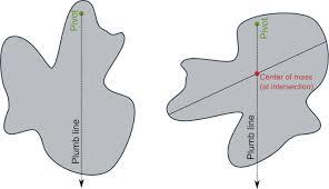
Fig. 9: Plumb Line Model Of Gravity Center of Mass Action. This concept is extremely important for all of the future derivations in this paper.
33
T = 2π ( 2.2 ⋅ 10 20 m) 230, 000 m / s = 6.01 ⋅ 1015 sec
With Kepler’s Third law we can calculate the mass of the galaxy:
MWith a radius from the center of our galaxy of , Gravitational Constant and an orbital period of we have a mass of galaxy of
To calculate the centripetal acceleration of the sun in our galaxy we can do the following:
The centripetal acceleration produced by the suns velocity and radial distance:
The gravity produced if all the milky ways galactic mass is considered to be concentrated at the center of the galaxy in the central black hole (Sagittarius A).
Thus, we conclude that all of the energy produced by the strings work is accounted for. Consequently, we can further demonstrate in a series of examples that the gravitational energy produced by the center of mass of bodies is sufficient to explain all gravitational effects in the universe.
We can begin by analyzing the Moon – Earth gravitational System:
The orbital velocity is: The average Orbital Radius is:
34
galaxy
4π
r
GT
6.01
1.743762874
41 kg acentripetal = GM r 2 v 2 r = GM r 2 v
GM
=
=
2
3
2 2.2 i1020 meters G = 6.67408 i 10 11 m 3 / kg ⋅ s 2
i 1015 sec
i 10
2 r = ( 230, 000 m / s ) 2 ( 2.2 i 10 20 m) = 2.404545455 i 10 10 m / s 2
r 2 = ( 6.67408 i 10 11 m 3 / kg i s 2 ) i (1.743762874 i 10 41 kg ) ( 2.2 i 10 20 m) 2
2.404548124 i 10 10 m / s 2 1.022 i 103 m / s 384, 400, 000 meters
Thus, the centripetal acceleration of the moon is:
In this simple system, the gravitational acceleration of the earth-moon system is sufficient to explain the gravitational effects displayed by the Moon Earth System: acentripetal moon = v 2 r = (1.022 i 103 m / s ) 2 ( 384, 400, 000 m) = 2.717180021 i 10 3 m / s 2
Earth r 2 = ( 6.67408 i 10 11 m 3 / kg i s 2 )(5.972 i 10 24 kg ) ( 384, 400, 000 m) 2
2.697394385 i 10 3 m / s 2
35
GM
=
12. Solving the Dark Matter/Energy puzzle.
I set out to explain the center of gravity action problem. I postulated that this would mean that the black hole was absorbing all of the Milky Ways galaxies energy. Consequently, I realized that since all of the Milky Ways galaxies energy is concentrated on the black hole, then, this is the primary reason for the formation of black holes in the center of galaxies.
I further taught that the gravitational signal had to be traveling bi-directionally. One way with all the Milky way galactic elements concentrating their energy on the black hole. And then the black hole re-radiates its gravitational energy back to the stars. However, when I looked at close stars that were orbiting Sagittarius A* I found that the mass that they experienced was that of the sphere they were orbiting in: on the order of .
kg
In other words, the radius at which they orbited, accounted for the mass that they felt (as previously predicted by normal gravitational considerations).
For Example: Star S1 which orbits Sagittarius A*
The orbital velocity at the pericenter is:
v = 1, 648, 858.519 m / s
Its radius is 2160.7 AU.
r = 3.232361192 i 1014 meters
Orbital Period Is 166 years or
t = 5.234976 i 109 sec
Gravitational Constant:
G = 6.67408 i 10 11 m 3 / kg ⋅ s 2 M star = 4π 2 r 3 GT 2 = 7.289 i 1035 kg
And the calculated mass of star S1 is as follows.
41 kg
The mass of the galaxy is in the order of . Thus, I concluded that there must be a mechanism for the cancelation of the energies if my assumption that all the mass of the galaxy is supposed to be acting on the center of as seen on the moon and our sun.
36
1035
10
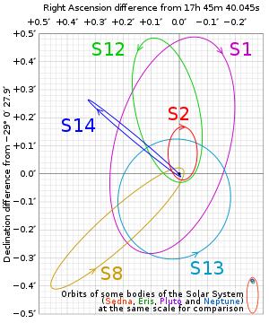
Fig. 10: A few stars Orbiting Sagittarius A*
As shown by: Eisenhauer, F.; et al. (July 20, 2005). "SINFONI in the Galactic Center: Young Stars and Infrared Flares in the Central Light-Month". The Astrophysical Journal. 628 (1): 246–259 [16]
Thus, the total energy I concluded must be equal to the gravitational energy provided by the black hole (with the entire mass of the galaxy at the center) minus the work done on the orbiting star from a radius larger than that of the star orbiting the Sagittarius a* .
37
I assumed that the centripetal energy is equal to the gravitational energy of the star minus the work to the edge of the galaxy.
Where the acceleration is produced by the gravitational potential energy density of the galaxy.
Simplifying we get:
The stars I used to calculate the energetics are found in the Wikipedia entry of Sagittarius A*. https://en.wikipedia.org/wiki/Sagittarius_A* [17] mv
And solving for the distance that the work is being performed, should yield the size of the galaxy, but as our calculations will soon show, it actually yields the distance to the edge of the universe.
38
star
star
star
star
star
star
star
GM Galaxy r star
star
xuniverse
GM Galaxy r star v star 2 ⎛ ⎝ ⎜ ⎞ ⎠ ⎟ GM Galaxy r sun 2 ⎛ ⎝ ⎜ ⎞ ⎠ ⎟
star 2 r star = GM Galaxy m r
2 m a x galaxy mv star 2 r
r
= GM Galaxy m r
2 r
m a x galaxy a = GM Galaxy r sun 2 v
2 = GM Galaxy r
a ⋅ x galaxy a ⋅ x galaxy =
v
2
=
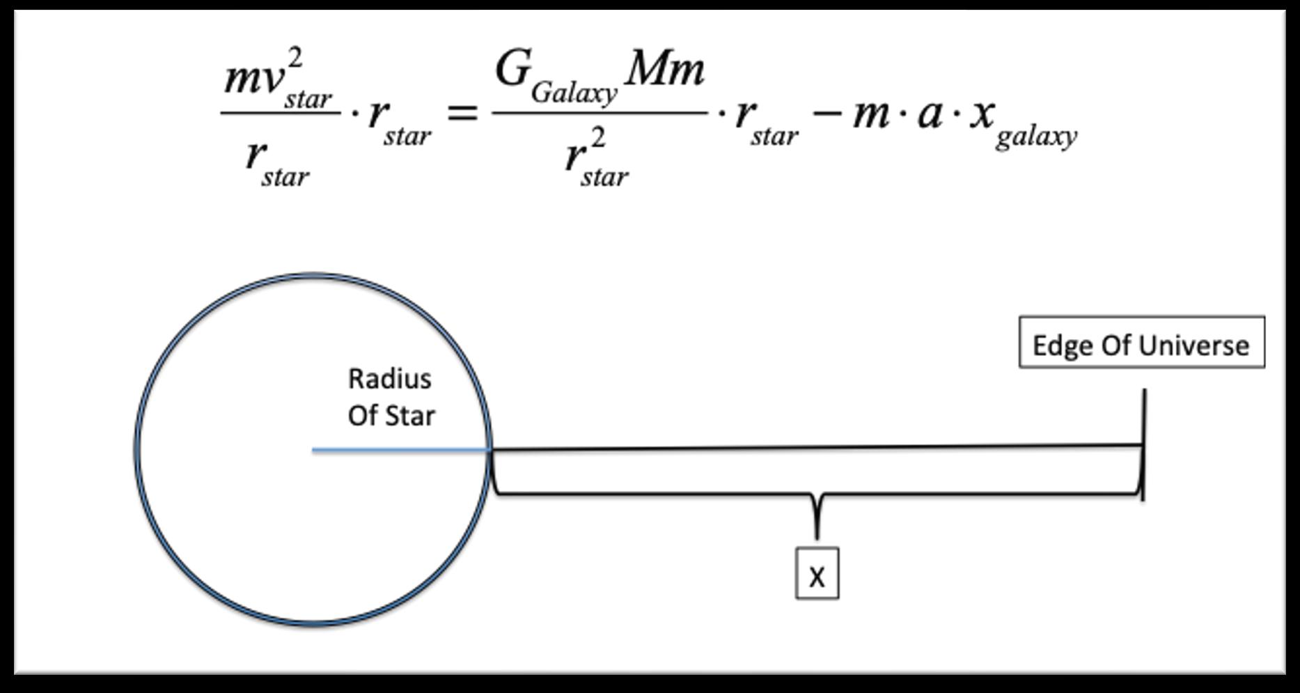
Fig. 11: The Energy of a star is given by the Gravitational Potential minus the work of Dark Energy.
The following are the calculations I performed to measure the distance of the universe using stellar energetics.
It is important to note that I choose star S1 orbiting Sagittarius a* to have the correct age of the universe. And this yielded a distance of the universe as follows:
G = 6.67408 i 10 11 m 3 / kg ⋅ s 2
M Galaxy = 1.743762874 i 10 41 kg
The orbital velocity at the pericenter of star S1 is:
v = 1, 648, 858.519 m / s
r sun = 2.2 i 10 20 m
r star = 2160.7 AU = 149, 597, 870, 691m / AU ( ) 2160.7 AU ( )
= 3.232361192 1014 m
xuniverse
39
GM Galaxy r star v star 2 ⎛ ⎝ ⎜ ⎞ ⎠ ⎟ GM Galaxy r sun 2 ⎛ ⎝ ⎜ ⎞ ⎠ ⎟
=
We can assess the output by calculating the terms individually.
3.600467965 i 1016
2.404548124 i 10 10 m / s 2 xuniverse = 1.497244349 i 10 26 m tuniverse = xuniverse / c = 4.994269566 i 1017 sec tuniverse = 4.994269566 i 1017 sec ( 3600 s )( 24 hours )( 365) = 15.8367249 i 109 years
Thus the age of the universe measured as previously stated was calculated to be:
15, 836, 724, 903 years
Our colleagues measured the age of the universe based on the WMAP data to be 13.772 billion years old. The measurement that I performed is 15.8 billion years using stellar energetics. However, a theoretical estimation of the universe, using a heat equation of proton rest mass energy, will prove the theoretical age of the universe in section 16 of this paper to be in close agreement. GM Galaxy
Inputting all these numbers into the equation we find the size of the universe and the time since the big bang as follows:
40
GM
r sun
=
kg s 2
kg
(
20 m
r star = ( 6.67408 i 10 11 m 3 / kg s 2 ) i (1.743762874 i 10 41 kg ) ( 3.232361192 i 1014 m) =
m 2 / s 2 v star 2 = (1648858.519 m / s ) 2 = 2.718734416 i 1012 m 2 / s 2
Galaxy
2
(6.67408 i 10 11 m 3 /
) i (1.743762874 i 10 41
)
2.2 i 10
) 2 =
After studying the data set produced by all the stars I noticed that there are inflationary effects in the data. Thus it is possible with astronomical observations to prove inflation.
For most of the stars, the distances in the data for the edge of the universe calculation were in the order of magnitude of which is an expected value based on all visual observations of the farthest galaxy. MACS0647-JD is 13.3 billion light-years away. Which corresponds with an observable order of magnitude of
10 26 meters 10 24 meters
Due to inflationary effects in my data set, I noticed that the range of the values I received were an order of magnitude smaller or larger than the size of the universe, or to
10 25 meters 10 27 meters
41
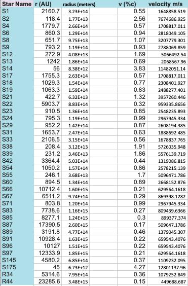
Table 6: Velocity and Radius are taken at the pericenter to have maximum centripetal energy. A percent of the speed of light expresses the velocity of the star.
42
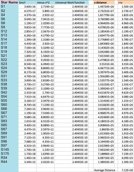
Table 7: The energetics of the star orbiting Sagittarius a* were calculated using the energetic difference calculation. The distance of the universe was calculated.
43
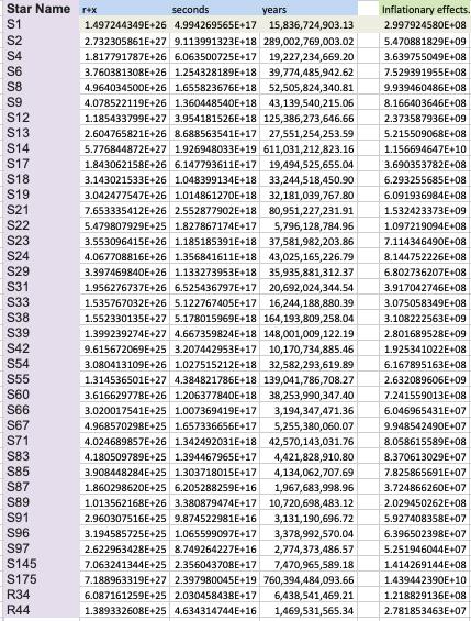
Table 8: I choose the 15.8 billion year age to calculate the Inflationary effects, and we can notice that the light travels slower and faster than the speed of light in other stars signals due to inflationary effects.
44
Another technicality that I want to discuss is as follows.
If you notice the acceleration term given was calculated from the center of the black hole (sagitarrius a*) to the sun. This is because the universe energy is isotropic and homogenous, so their is an even energy distribution from the sun to the edge of the universe. One of the reasons for this is due to the fact that matter waves traveled at the speed of light before they clumped up into subatomic particles, so this creates a homogenous energy distribution in every linear dimension perpendicular to the centripetal acceleration of the galactic star throughout the edge of the universe:
As predicted by Stephen Hawking (1966). “Properties of expanding universes “ (Doctoral thesis)[18].
With astronomical data we can also prove inflation as follows:
If we take the size of the universe to be then it means that there must be a fixed time at which all the light energy traveled. And we can use this as a baseline to measure inflationary effects as seen in Table 8.
Thus our reference time, the time since the big bang is as follows.
= 1.497244349 10 26 m t s tan dard = x / c = 1.497244349 E + 26 m 299792458 m / s = 4.994269566 E + 17 sec
v = x t s tan dard = c
However other signals traveled more distance due to inflationary effects and changes in the geometry of space itself. As in the case of Star R44s work function data, as seen in Table 7.
v = xother t s tan dard
45
a = GM Galaxy r sun 2 x
Star R44 Orbiting Sagittarius A*
v = xother t s tan dard = 1.38933 10 25 m 4.994269566 ⋅ 1017 s
= 2.7818482 107 m / s
Thus space contracted for star R44 as the measured distance of work is smaller based on the measured energetics of the star. It ran at the speed of light, but due to space contraction, it had an effective relative speed of 9.28% the speed of light.
Star S14 Orbiting Sagittarius A*
The fastest light signal measured was that of star S14
v = xother t s tan dard = 5.77684 10 27 m 4.994269566 ⋅ 1017 s
= 1.156693671 1010 m / s
Which runs faster than light, at 38.6 times the speed of light, as Space expanded to produce the inflationary effect observed.
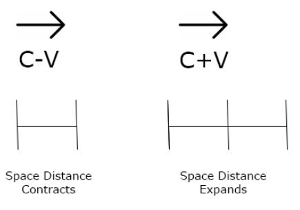
Fig. 12: Inflationary Effects were seen in the data speed and slow the light signals.
Thus I conclude that the inflationary effects that I measured change the geometry space with signals traveling 9.27% the speed of light to fast as 386% the speed of light.
46
13. Black Holes
We can calculate the size of a black hole radius by using the derivation of the Schwarzschild Radius.
1
2 mv 2 = GMm r
1
2 c 2 = GM r
r = 2GM c 2
M galaxy = 1.473760938 i 10 41 kg
G = 6.67408 i 10 11 m 3 / kg ⋅ s 2
c = 299, 792, 458m / s
Where the radius of our black hole is:
r s = 2GM c 2 = 2 i ( 6.67408 i 10 11 m 3 / kg i s 2 )(1.473760938 i 10 41 kg ) ( 299792458 m / s ) 2 = 2.188804834 i 1014 meters
The mass of the galaxy determines the size of the galaxy’s black hole. And the speed of light is fundamental for galactic formation.
Stephen Hawking derived the energy of a black hole by inputting the Schwarzchild radius in the gravitational equation as follows:
rs = 2GM c 2
g = GM rs2 = c 4 4GM
M galaxy = 1.473760938 i 10 41
g = c 4 4GM Galaxy = 205.3m / s 2
E = hf 2π fc g
47
E = h 2πc g
Stephen Hawking took the ratio of the acceleration of a black hole ratio to the string theory acceleration (but he didn’t have the full expression of string theory and he didn’t have the frequency terms in his expression). However, If you plug in the numbers we find that it yields an acceleration that is too small to be that of a black hole (205.3m/s^2). So I figured that STEPHEN HAWKINGS solution must not be correct. Because the Sun’s gravity is 274 m/s^2 and black holes have more than one sun’s gravitational potential. And as we previously explained the entire mass of the universe gravitational energy is concentrated at the center of the black hole.
Luckily, I had derived a different solution that explains black holes better. String theory must be taken into account to solve this issue due to the concentration of large energies at the center, due to the center of mass action.
The work of gravity in the black hole from the center to the exterior event horizon is equal to the kinetic energy. And this yields the frequency of light strings at the event horizon.
GMm
r 2 i r = mv 2 2
GMm
r = m 2 i x 2 t 2
2GM
r 3 = 1 t 2
M galaxy = 1.473760938 i 10 41 kg
G = 6.67408 i 10 11 m 3 / kg ⋅ s 2
c = 299, 792, 458m / s
f = 2GM r 3 = 2GM ( c6 ) ( 2GM )3 =
i 10 6 hz
48
G 3 M 3 = c6 4G 2 M 2 = 1.36966281
GMc6 4
hf = 3 2 kT
f = 1.36966281 ⋅ 10 6 Hz
h = 6.62607004 i 10 34 m 2 kg / s
k = 1.38064852 i 10 23 m 2 kg / s 2 K
If we want to calculate the temperature of a black hole at the surface in the event horizon we can use the following expression: s
T = 2 hf 3k = 4.382231286 i 10 17 K T
The radiation of a black hole is as follows:
4 = 16πG 2 M 2 c 4 ⎛ ⎝
And thus we have verified the well-known fact that black holes are black. This calculation demonstrates that fact!!!
49
2
hf k B
2 3 h k B c 6 4G 2 M 2 ⎛ ⎝ ⎜ ⎞ ⎠ ⎟
4π ( 2GM c 2
2 = 16πG 2 M 2 c 4 σ
π 5 k B 4 15
P
P = 16πG 2 M 2 c 4 ⎛ ⎝ ⎜ ⎞ ⎠ ⎟ 2π 5 k B 4 15c 2 h 3 ⎛ ⎝ ⎜ ⎞ ⎠ ⎟ 2 3 h k B c 6 4G 2 M 2 ⎛ ⎝ ⎜ ⎞ ⎠ ⎟ ⎛ ⎝ ⎜ ⎜ ⎞ ⎠ ⎟ ⎟
⎜ ⎞ ⎠ ⎟ 2π 5 k B 4 15c 2 h 3 ⎛ ⎝ ⎜ ⎞ ⎠ ⎟ 16 81 h 4 k B 4 c 12 16G 4 M 4 ⎛ ⎝ ⎜ ⎞ ⎠ ⎟ ⎛ ⎝ ⎜ ⎞ ⎠ ⎟ = 2π 6 k B 4 15h 3 ⎛ ⎝ ⎜ ⎞ ⎠ ⎟ 16 81 h 4 k B 4 c 6 G 2 M 2 ⎛ ⎝ ⎜ ⎞ ⎠ ⎟ ⎛ ⎝ ⎜ ⎞ ⎠ ⎟ = 2π 6 15 ⎛ ⎝ ⎜ ⎞ ⎠ ⎟ 16 81 h ⎛ ⎝ ⎜ ⎞ ⎠ ⎟ c6 G 2 M 2 ⎛ ⎝ ⎜ ⎜ ⎞ ⎠ ⎟ ⎟ =
6 1215G 2 M 2 = 1.258972597
10 43 watts
=
3
=
A = 4π r 2 =
)
= 2
c 2 h 3
= AεσT 4
32π 6 hc
i
To calculate the acceleration of matter at the Schwarzschild Radius we need to use the following expression from string theory.
a c = 2π fc = 2π i (1.36966281 i 10 6 hz ) i ( 299792458 m / s ) = 2580 m / s 2
We can further study the dynamics inside of a black hole. If we compute the work done from the edge of a black hole (the event horizon) to the center we can compute the kinetic energy.
r s = 2GM c 2
M galaxy = 1.473760938 i 10 41 kg
f = 1.36966281 i 10 6 hz
G = 6.67408 i 10 11 m 3 / kg s 2
c = 299, 792, 458m / s
max = mv 2 2
m( 2π fc ) x = mv 2 2
r s = 2GM c 2
However, due to time dilation, the signal travels at the speed of light inside of the black hole.
If we use the mass of a black hole as currently measured by my colleagues in the paper titled “An Improved Distance and Mass Estimate for Sgr A* from a Multistar Orbit Analysis by A. Boehle et al.” [19]
v = 2( 2π fc ) R s = 2( 2π fc )( 2GM ) c 2 = (8π fGM ) c = 1.062736593 i 109 m / s mbh = 7.99545 i 1036 kg
Namely, 4.02 million solar masses or . A figure that is less than the whole galaxy mass.
50
We would get the following:
f = c 6 4G 2 M bh 2 = 0.02524630318 Hz
And the acceleration calculated would be:
a = 2π fc = 47 , 555, 238.55
However, this acceleration I believe is too large. And in later chapters, we will demonstrate that breaking down the electrostatic force in the black hole requires a larger energy density in the black hole.
Comparatively, if you recall I measured the acceleration to be
2580 m / s 2
We calculate the velocity at the event horizon as follows:
a = 2π fc
f = a 2π c = 2580 m / s 2 2π i 299792458 m / s = 1.36968 i 10 6 hz
We can calculate the velocity of a proton at the event horizon.
m proton = 1.6726219 i 10 27 kg
h = 6.62607004 i 10 34 m 2 kg / s
f = 1.36966281 i 10 6 hz
E = hf = 3 2 KT = 1 2 mv 2
Vschwarzschild = 2( hf ) m proton = 1.041726415 ⋅ 10 6 m / s
r proton = 0.21 10 15 m
With this result, we notice that the particle moves slowly at one proton radius per 2.01E10 seconds. Typical rates for hydrogen at room temperature are 1,754 m/s. Or it moves one proton radius in 1.197E-19 seconds. So ironically black holes are “cold” at the event horizon.
51
14. Deriving the Mass of the Universe using astronomical data.
If you recall we measured the galaxy mass to be
M galaxy = 1.473760938 i 10 41 kg
This is the mass I believe to be acting on Sagittarius a*.
If this were to be true the Schwarzschild radius is.
r s = 2GM c 2 = 2 i ( 6.67408 i 10 11 m 3 / kg i s 2 )(1.473760938 i 10 41 kg ) ( 299792458 m / s ) 2 = 2.188804834 i 1014 meters
My colleagues believe the mass of the black hole is on the order of 8.4727992e+36 kg. As found in “An Update on Monitoring Stellar Orbits in the Galactic Center” by Gillessen et al. Or “Monitoring Stellar Orbits Around the Massive Black Hole in the Galactic Center” by Gillesen et al.(2018)]
r s = 2GM c 2 = 2 (6.67408 10 11 m 3 / kg s 2 )(8.4727992 1036 kg ) ( 299, 792, 458 m / s ) 2 = 1.25836 1010 meters
At first glance, the Schwarzschild radius distance calculated by my colleagues seems to be correct given that there are stars observed at the radi as close as . Such as star S14, or star S175. Even star s2 whose orbit has been carefully studied orbits at a radius on the order of magnitude of . A gas cloud moving on the edge of Sagittarius a* has also been carefully studied. Such as in the paper: “A gas cloud on its way toward the super-massive black hole in the Galactic Center” published by S.Gillessen et al.(2012) [21]
1012 meters
1013 meters
Previously I proposed that our black hole has a Schwarzschild radius on the order of magnitude of . Essentially, all of the stars I used to prove the mechanism of gravity would be eaten by the black hole at this value. That presented a problem. But given the overwhelming evidence that gravity acts on the center of mass given the energetic calculations of stars, the sun’s core temperature, the earth’s core temperature, and the gravitational mechanism to hold hurricanes together. Given all of this evidence it’s important to not discard this hypothesis quickly as an explanation for the elusive dark energy.
1014 meters
52
The solution lies in the fact that the black hole, Sagittarius A*, shrunk with the work done on it by the entire universe.
My colleagues measured the experimental value of the Schwarzschild radius in the following in the paper titled “Detection of intrinsic source structure at ~3 Schwarzschild radii with Millimeter-VLBI observations of SAGITTARIUS A*” by Ru-Sen Lu et al [22]. In this paper, my colleagues measured the Schwarzschild radius to be 10 Micro arc seconds.
Given these experimental results as well as the fact that orbiting stars and gas clouds orbit our galactic black hole at a smaller radius, we can consequently infer, and prove by my future calculations, that the black hole shrunk from its original radius to a smaller radius on the order of magnitude of . Dark energy from the entire universe did work on the black hole to shrink it to a smaller size.
1010 m
1014 m
The Schwarzschild radius can be calculated using the arc length measurement cited in the previous paper as well as using the distance to our galactic center.
θ = 10µas = 10 i 10 6 arc sec ond = ( 1! 3600 )(10 i 10 6 )( π 180! )
= 4.848136811 i 10 11 rad
rschwarzschild = rsagittarius a* i θ
rschwarzschild = ( 2.2 i 10 20 m)( 4.848136811 i 10 11 rad )
= 1.066590098 i 1010 m
53
Thus, using this value we can calculate the mass of the universe as follows:
mv 2
rschwarzschild = GM Galaxy m rschwarzschild 2 m ⋅ a ⋅ xuniverse
mv 2
rschwarzschild ⋅ rschwarzschild = GM Galaxy m rschwarzschild 2 ⋅ rschwarzschild m ⋅ a ⋅ xuniverse
mv 2 = GM Galaxy m rschwarzschild m ⋅ a ⋅ xuniverse
Recall that,
a i x = a i runiverse = M UniverseG runiverse 2 i runiverse = GM Universe runiverse
Where this is the theoretical energy of all dark energy in the universe!
Thus,
vschwarzschild 2 = M Galaxy G rschwarzschild ( GM Universe r universe 2 ) i runiverse
Reshuffling the terms to solve for the mass of the universe we get the following:
M Galaxy G rschwarzschild vschwarzschild 2 = ( GM Universe runiverse )
M Universe = ( M Galaxy G rschwarzschild vschwarzschild 2 )( runiverse G )
M Universe = ( M Galaxy G rschwarzschild vschwarzschild 2 )( runiverse G )
54
We can calculate the individual terms and use the constants to solve for the mass of the universe as follows.
G = 6.67408 i 10 11 m 3 kg / s 2
M Galaxy G
rschwarzschild = (1.473760938 i 10 41 kg )(6.67408 i 10 11 m 3 / kg i s 2 ) (1.066590098 i 1010 m)
= 9.221910479 i 10 20 m 2 / s 2
vschwarzschild = 1.041726415 10 6 m / s
vschwarzschild 2 = 1.085193924 ⋅ 10 12 m 2 / s 2
runiverse G = (1.49724 i 10 26 m) ( 6.67408 i 10 11 m 3 kg / s 2 ) = 2.243365378 i 1036 m
Thus using all of these values we find that the measurement of the mass of our universe is:
M universe = 2.068811468 ⋅ 1057 kg
55
15. Proving the acting mechanism of Dark Energy and the Size of the universe using electrostatic and gravitational considerations in the core of our sun.
In a black hole, the electrostatic forcé breaks down because everything inside the black hole moves at the speed of light.
1.36966281 10 6 Hz λ = 2.188 1014 Hz
Recall that the frequency of light in the event horizon is . Thus, the wavelength of the light at this frequency is . However, since the light is not baryonic, as proved by the wavelength of light in the event horizon, the electrostatic force has to break down in black holes.
Recall the theoretical size of the proton is as follows:
r proton = 2.1 i 10 16 m
k e = 8.9875517887 i 109 Nm 2 / C 2 q = 1.602 i 10 19 C Felectrostatic = k e qq ( 2 r proton ) 2 = (8.9875517887 i 109 Nm 2 / C 2 )(1.602 i 10 19 C )(1.602 i 10 19 C ) (( 2) i ( 2.1 i 10 16 m)) 2
If we consider the electrostatic force between to adjacent protons, from proton center-tocenter, we get the following.
= 1307.578734 Newtons
56
Thus, we can derive the mass required to break down the electrostatic forcé for a pure black hole signal to form.
F gravity = Felectrostatic
GM sun m proton r sun 2 = k e qq ( 2 r proton ) 2
Solving for the mass required to break down the electrostatic forcé we find something astonishing.
m proton = 1.6726219 i 10 27 kg
G = 6.67408 i 10 11 m 3 kg 1 s 2
r sun = 6.9551 i 108 m M Sun = k e qq i r sun 2 ( 2 r proton ) 2 i G i m proton = (1307.578734 N )( 6.9551 i 108 m) 2 ( 6.67408 i 10 11 m 3 kg 1 s 2 )(1.6726219 i 10 27 kg )
To form a black hole you dont need 1.4 times the mass of the sun, as predicted by the Chandrasekhar limit, you need to concentrate the mass of the galaxy, and an additional net center of mass of the universe. Collectively the center of mass to form a black hole should be as great as the mass in the universe (as shown below)!
= 5.666115448 i 1057 kg M Universe = 5.666115448 i 1057 kg M Universe = 2.068811469 i 1057 kg
Previously, using the energetics of the black hole, and the stars orbiting Sagittarius A*, we estimated the mass to be as follows
57
16. Proving the cosmological evolution of the universe and The Equation of the Big Bang using Infinite Spatial Domains and an Infinite Rod Thermal Distribution.
The following is the derivation of all matter states based on matter phase state transitions.
We Begin by solving the Heat Kernel. Which while provide us the solution to study the distribution of heat in the universe I used the following two papers. Deriving the Heat Kernel in 1 Dimension by Ophir Gottliev [23] and Infinite Spatial Domains and the Fourier Transform by Matthew J. Hancock [24]
58
Fig. 13 the Cosmological Evolution of the Universe
The solution for the heat kernel is as follows:
γ = 1 t
α = β = 1 t
G ( x , t ) = 1 t Q ( ε )
ε = x t
G t = k ΔG
G t = 1 2 t 3 2 Q 1 2 t 3 2 ( t 1 2 x )Q '
G t = 1 2 t 3 2 Q 1 2 t 3 2 ( ε )Q '
G t = 1 2 t 3 2 ( Q + εQ ')
G xx = t 3 2 Q '' 1 2 t 3 2 ( Q + εQ ') = kt 3 2 Q ''
Q + εQ '+ 2 kQ '' = 0
( εQ ) '+ 2 kQ '' = 0
εQ + 2 kQ ' = c
Now we note that we expect . Consequently, we expect as . Therefore c = 0. We have the ODE
G ( ∞ , t ) = 0 Q ' = 0 x → ∞
εQ + 2 kQ ' = 0
2 kQ ' = εQ
Q ' = εQ 2 k
Q Q ' = ε 2 k
59
Integrating and simplifying we get:
Where creates the initial function.
As the Velocity Increases the heat radiation diminishes. Where x is the velocity of the matter particle. As the velocity decreases radiation acceptance increases.
We can solve for the initial constant as follows.
Given a probability distribution, by conservation of energy and probability theory says that the probability distribution is equal to one when the curve is integrated, we find.
Plugging in for t, and solving for the Gaussian Function we get:
60
k
( ε
Ce ε 2 4 k t = 1 4 k
ε
Ce x 2 4 kt Q
x → Q Q
Ce x 2 4 kt t Q ( x
t
1 ∞ ∞ ∫ Ce x 2 4 kt t = 1 ∞ ∞ ∫ t = 1 4 k 4 k Ce x 2 = 1 ∞ ∞ ∫ e x 2 = π ∞ ∞ ∫ 4 kπ C = 1 C = 1 4 kπ
ln Q = ε 2 4
+ C Q
) =
Q (
) =
→ x
( x , t ) =
,
) =
For . When there is no heat transfer, When Q = 0, When , the mass has a definite energy value.
ln Q = ε 2 4 k + C e ∞ = 0
When Q = 0, When ,
ε 2 4 k = C C = 1 4 kπ ε 2 4 k = 1 4 kπ
ε 2 = 4 k 4 kπ = 4 k π k = 1 16π
ε 2 = 1 2π
ε = x t x 2 t = 1 2π
x 2 = t 2π v = x = t 2π
This result is very important because x is really the speed of the signal.
And thus the Energy of a particle is stable without the presence of heat. Thus, proton decay is not possible. Q ( x , t ) = e x 2 4 kt 4 ktπ C = 1 4 kπ e ∞ = 0
61
We will use this result to derive the kinematic equations of the universe at the end of this paper.
Johann Carl Friedrich Gauss derived the following expression which we will use to derive the equation that describes the energetic distribution of the entire universe.
Let,
We can use the definition of Gauss’s Error Function to multiply by square root of pie over two. u
62
( x , t ) = f ( s ) 4 kπt e ( x s )2 4 kt ⎛ ⎝ ⎜ ⎞ ⎠ ⎟ ∞ ∞ ∫ ds = u o ε 4 kπt e ( x s )2 4 kt ⎛ ⎝ ⎜ ⎞ ⎠ ⎟ ε / 2 ε / 2 ∫ ds
4 kt
( x
t ) = u o ε π e z 2 x ε / 2 x + ε / 2 ∫ dz = u o ε π e z 2 0 x + ε / 2 4 kt ∫ dz + e z 2 x ε / 2 4 kt 0 ∫ dz ⎡ ⎣ ⎢ ⎢ ⎤ ⎦ ⎥ ⎥ = u o ε π e z 2 0 x + ε / 2 4 kt ∫ dz e z 2 0 x ε / 2 4 kt ∫ dz ⎡ ⎣ ⎢ ⎤ ⎦ ⎥
z = ( x s ) /
4 kt ( ) dz = ds u
,
erf ( x ) = 2 π e x 2 0 x ∫ dx
π 2 i erf ( x ) = e x 2 0 x ∫ dx u ( x , t ) = u o 2
Using the definition of the integral we solve:
Using the definition of the Gauss error function:
We get:
erf ( z ) = 2 z π e z 2 u ( x , t ) = u o ε 4π kt ( x + ε 2 ) exp ( x + ε / 2) 2 4 kt
= u o ε 4π kt ( ε 2 ) exp ( x + ε / 2) 2 4 kt
⎣ ⎢ ⎢
Where K is part of an acceleration constant.
⎦ ⎥ ⎥ k = 1 16π x = c ε = c
Where epsilon is the three-dimensional speed of light.
ε = v t = D t 2 / 2 t 1/ 2 = D t 3/ 2 = c
63
⎤ ⎦ ⎥
ε erf ( x + ε / 2 4 kt ) erf ( x ε / 2 4 kt ) ⎡ ⎣ ⎢
⎞
ε
kt ⎛ ⎝ ⎜ ⎞ ⎠ ⎟ ⎡ ⎣ ⎢ ⎢ ⎤ ⎦ ⎥ ⎥
⎠
⎛ ⎝ ⎜ ⎞ ⎠ ⎟ ⎛
⎞ ⎠
⎡
⎤ ⎦
⎛ ⎝ ⎜ ⎞ ⎠ ⎟ ⎛
⎞ ⎠
⎡
⎛ ⎝ ⎜
⎠ ⎟ ( x ε 2 ) exp ( x
/ 2) 2 4
⎛ ⎝ ⎜ ⎞
⎟ + exp ( x ε / 2) 2 4 kt
⎝ ⎜
⎟
⎣ ⎢ ⎢
⎥ ⎥ = u o 2 4π kt exp ( x + ε / 2) 2 4 kt ⎛ ⎝ ⎜ ⎞ ⎠ ⎟ + exp ( x ε / 2) 2 4 kt
⎝ ⎜
⎟
⎤
v = x = t 2π
However, since it’s a light signal the velocity simplifies to c.
x = v = c Plugging in for epsilon and x
=
exp
u o t exp ( 2 c 2 + c 2 / 4) i 4
⎢
= u o t exp (9 c 2 / 4) i 4π t ⎛ ⎝ ⎜ ⎞
= u o t exp (9 c 2 / 4) i 4π
⎛ ⎝ ⎜ ⎞ ⎠ ⎟ + exp ( c 2 / 4) i
= u o t exp (9 c 2 ) i π
Which yields, The Heat Equation of The Universe
u ( x , t ) = u o t 3/ 2 exp (9 c 2 ) i π
It is important to note that the time is cubed because we are considering the heat diffusion in 3 dimensions. It is also important to understand that heat and kinetic energy are interchangeable.[25] http://hyperphysics.phy-astr.gsu.edu/hbase/Kinetic/maxspe.html#c2
This energy is derived from God’s infinite reaches.
If we plug in the energy of the big bang and the time I calculated for the age of the universe, we can calculate today’s Protons Energy.
64
(
c
2) 2 i 4π t ⎛ ⎝ ⎜ ⎞ ⎠ ⎟ + exp ( c c / 2) 2 i 4π t ⎛ ⎝ ⎜ ⎞ ⎠ ⎟ ⎛ ⎝ ⎜ ⎞ ⎠ ⎟ ⎡ ⎣ ⎢ ⎢ ⎤ ⎦ ⎥ ⎥
(
2 + c 2 + c 2 / 4) i 4π t ⎛ ⎝ ⎜ ⎞ ⎠ ⎟ + exp ( c 2 c 2 + c 2 / 4) i 4π t ⎛ ⎝ ⎜ ⎞ ⎠ ⎟ ⎛ ⎝ ⎜ ⎞ ⎠ ⎟ ⎡ ⎣ ⎢ ⎢ ⎤ ⎦ ⎥ ⎥
u ( x , t )
u o t
c +
/
= u o t exp
c
t
⎝ ⎜ ⎞ ⎠
exp
π t ⎛ ⎝ ⎜ ⎞ ⎠ ⎟ ⎛ ⎝ ⎜ ⎞ ⎠
⎣
⎠
4π t ⎛ ⎝ ⎜ ⎞ ⎠ ⎟ ⎛ ⎝ ⎜ ⎞ ⎠ ⎟ ⎡ ⎣ ⎢ ⎢ ⎤ ⎦ ⎥ ⎥
4π t ⎛ ⎝ ⎜ ⎞ ⎠ ⎟ ⎛ ⎝ ⎜ ⎞ ⎠ ⎟ ⎡ ⎣ ⎢ ⎢ ⎤ ⎦ ⎥ ⎥
⎠
π t ⎛ ⎝ ⎜ ⎞ ⎠ ⎟ ⎛ ⎝ ⎜ ⎞ ⎠ ⎟ ⎡ ⎣ ⎢ ⎢ ⎤ ⎦ ⎥ ⎥
π
⎛
⎟ +
( c 2 / 4) i 4
⎟ ⎡
⎢
⎤ ⎦ ⎥ ⎥
⎟ + exp ( c 2 / 4) i
t
t ⎛ ⎝ ⎜ ⎞
⎟ + exp ( c 2 ) i
t
⎞ ⎠
t ⎛ ⎝ ⎜ ⎞ ⎠ ⎟ ⎛ ⎝ ⎜ ⎞ ⎠ ⎟ ⎡ ⎣ ⎢ ⎢ ⎤ ⎦ ⎥ ⎥
⎛ ⎝ ⎜
⎟ + exp ( c 2 ) i π
e x 2 ∞ ∞ ∫ dx = π
u ( x , t ) = u o t 3/ 2 exp (9 c 2 ) i π t ⎛ ⎝ ⎜ ⎞ ⎠ ⎟ + exp ( c 2 ) i π t ⎛
At the beginning, the big bang signal started out as light and then it condensed to matter.
u o = c 2 = 2997924582 = 8.987551787 i 1016
t = (15.8 109 years )(365days )( 24 hours )(3600 sec onds ) = 4.982688 i 1017
⎟ = 0.56741374
t 3/ 2 = ( 4.982688 i 1017 )3/ 2 = 3.51718766 i 10 26 s
In 15.8 Billion years the energy of the particles cooled down throughout the age of the universe to:
u t = 1.4655 i 10 10 joules
The energy of a proton today is higher, so the time to diminish the energy should be smaller:
m proton = 1.6726219 i 10 27 kg
c 2 = 2997924582 = 8.987551787 i 1016
m proton c 2 = 1.503277595 i 10 10 joules
After plugging the time into the heat equation of the universe we found the elapsed time for the cooldown of the signal to today’s proton energy is 15.35 billion years.
t = 15.35 ⋅ 109 years
t = 4.840776 ⋅ 1017 sec
m proton c 2 = c 2 t 3/ 2 1 e 9 c 2 π
Thus we calculated the theoretical age of the universe previously with less than 3% error with the stellar energetics calculation.
65
⎝
⎞ ⎠ ⎟
⎞ ⎠
⎤ ⎦
⎜
⎛ ⎝ ⎜
⎟ ⎡ ⎣ ⎢ ⎢
⎥ ⎥
⎝
⎠ ⎟
t ⎛ ⎝ ⎜ ⎞ ⎠
exp (9 c 2 ) i π t ⎛
⎜ ⎞
= 0.006096752 exp ( c 2 ) i π
⎛
c
π t ⎛ ⎝ ⎜ ⎜ ⎞ ⎠ ⎟ ⎟ ⎡ ⎣ ⎢ ⎢ ⎢ ⎤ ⎦ ⎥ ⎥ ⎥
t
⎝ ⎜ ⎜ ⎞ ⎠ ⎟ ⎟ + 1 e
2
17. We can derive the dynamics of the Big Bang by using Unit Analysis and Electromagnetic Equations.
We can derive how long it took God to make all the mass in the universe as follows:
M bigbangparticle = 1
M bigbangparticle c 2 = hf resonant
c 2 = hf resonant
c 2 h = f resonant
The Poynting vector of light is as follows.
S = ExB µo
The units of the Poynting Vector units are as follows:
Thus the mass is as follows. Where t is the time it took God to create all the mass in the universe.
At first glance, it seems impossible to find this time, but after some clever thinking, it is in fact possible!
We can find the electric field if we know the energy in the signal.
66
⎡ ⎣ ⎢
⎦ ⎥
kg
m
m 2 ⎛ ⎝ ⎜ ⎞ ⎠ ⎟ = kg s 3 M universe = EB( t 3 ) µo t = M universeµo EB ⎛ ⎝ ⎜ ⎞ ⎠ ⎟ 1/ 3 B
E c t = M universeµo c E 2 ⎛ ⎝ ⎜ ⎞ ⎠ ⎟ 1/ 3
2
W m 2
⎤
=
i m i
s 3 i
=
U E = 1 2 ε E
U E = hf resonance E = 2 hf resonance
Where is the Permittivity constant.
i
Recall that is the following:
M Universe = 2.068811469 i 1057 kg
ε = 8.854 i 10 12 F / m
µo = 1.26 i 10 6 H / m
c = 299792458 m / s t = M
1/ 3 = 3.376448214 i 1010 s i ( 1hour 3600 s i 1day 24 hour i 1 year 365days ) = 1070 years
299792458)
Thus, based on the theoretical results from the calculation of universal energetics it took Big God 1070 years to make all the mass in the universe (based on all the experimental data that we have with the structure of Sagittarius a*).
Recall, that the electrostatic potential and gravitational potential yielded a lightly larger theoretical Mass value.
M Universe = 5.666115448 i 1057 kg
67
ε ε
ε 2 hf resonance ⎛ ⎝ ⎜ ⎞ ⎠ ⎟
f
ε = 8.854
10 12 F / m t = M universeµo c
1/ 3
resonance f resonance = c 2 h
2 c ⎛ ⎝ ⎜ ⎞ ⎠ ⎟
⎛ ⎝ ⎜ ⎞ ⎠ ⎟
universeµo ε
1/ 3 = ( 2.068811469 i 1057 kg )(1.26 i 10 6 H / m)(8.854 i 10 12 F / m) 2 i (
1/ 3 = (5.666115448 i 1057 kg )(1.26 i 10 6 H / m)(8.854 i 10 12 F / m) 2 i ( 299792458)
⎝ ⎜ ⎞ ⎠ ⎟ 1/ 3 = 4.72405481 i 1010 s i ( 1hour 3600 s i 1day 24 hour i 1 year 365days ) = 1498 years
Thus, this yields a mass aggregation time frame from 1070 years to 1498 years to make all the mass in the universe.
Next, we can calculate the size of the big bang signal as follows.
mc 2 = hf
m = hf c 2
c = d / t
m = ht 2 d 2t = ht d 2 = h cd
Recall that the signal had to be in resonance for the big bang energy to form. So m = 1. Solving for d we have:
h = 6.63 i 10 34 J s
c = 299, 792, 458 m / s
m = 1
This is the size of the diameter of the big bang signal with a constant signal adding energy with a resonant frequency. t = M universeµo ε 2 c
d = h c = 6.63 i 10 34 J s 299, 792, 458 m / s = 2.21 i 10 42 m
f resonance = c 2 h
68
⎝
⎛
⎜ ⎞ ⎠ ⎟
⎛
Recall that given the electrostatic and gravitational potential of Sagittarius a* the minimum theoretical time to make all the mass took 1498 years
t = 4.7240928 ⋅ 1010 s
Given this time if the signal was not resonant it would expand. We can see this result with the following derivation.
m = h cd
d = h cm = ht dm
d 2 = ht m
d = ht m
Recall that energy times time is the planck constant.
E = hf
Et = h
So,
d = Et 2 m
E = mc 2
d = c 2t 2 = ct
Using the theoretical time for the creation of the big bang. We can derive the distance of the signal would travel, if the signal were not resonating, and if God had released the signal continously while he was making the energy.
d = ( 299, 792, 458 m / s )( 4.7240928 1010 s ) = 1.416247392 1019 m
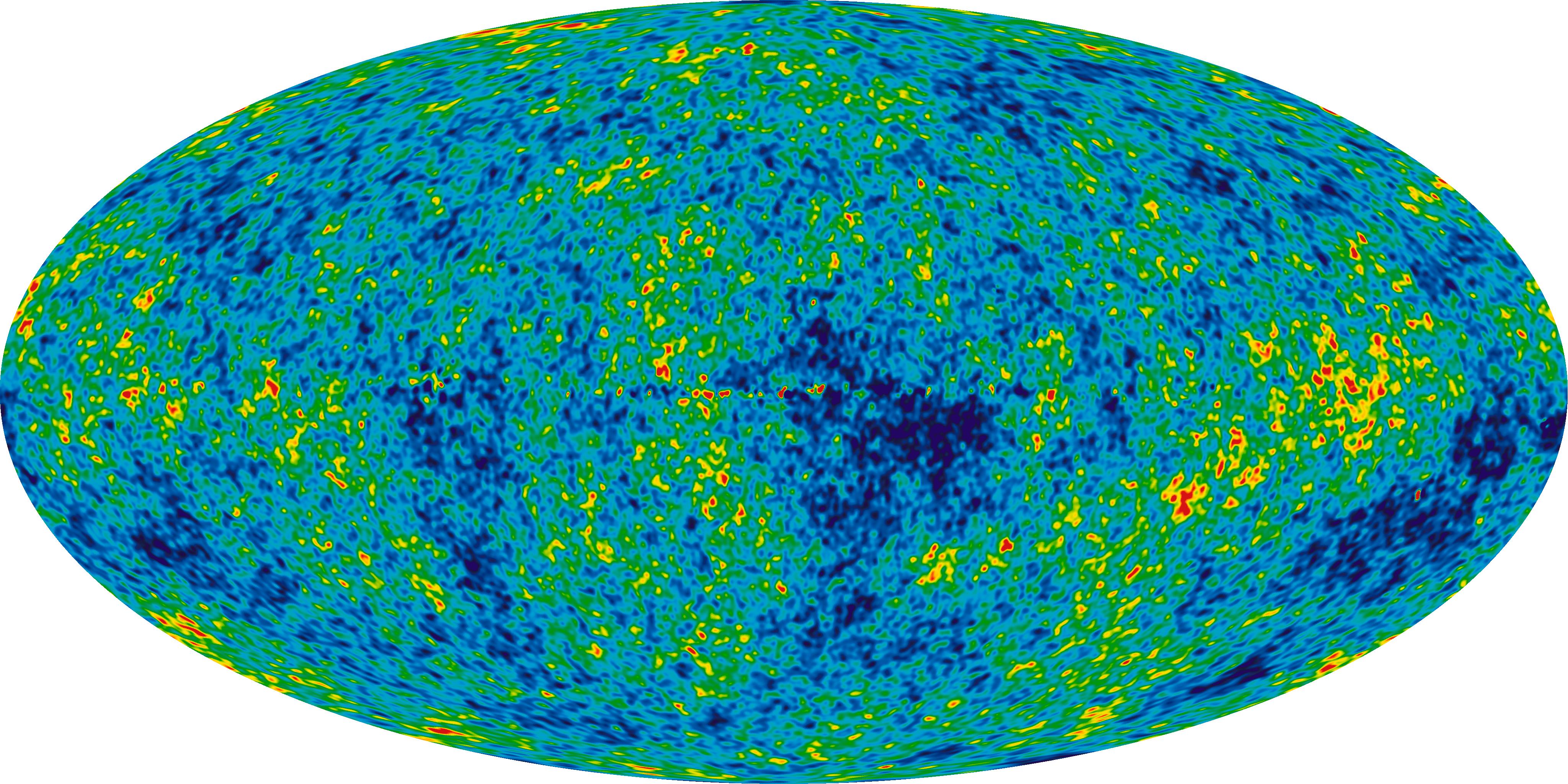
However, given the homogenous temperature distribution found in the cosmic background radiation, we can conclude that the big bang occurred in a singular event and not in a linearized release of energy.
69
The resonant frequency was created by GOD to create all the mass in the universe in a singular location.
If the energy had been released prior to the big bang, the temperature would be nonhomogenous due to proton cooling effects, and the size of the universe would be larger than the measured size of
x = 1.49724 E + 26 meters
70
Fig. 14: The Cosmic Microwave Background
18. We can derive all the kinematic equations from the heat equation definition as follows:
The kinematic variables are D (distance), V (velocity), a (acceleration), t (time), c (speed of light.
Where the Speed of Light is:
Recall that
v = x = t 2π
Where the Velocity is:
2 4 k = 1 4 kπ v = x = t 2
Where the Acceleration is: Where the
71
Distance is:
ε = v t = t 2π ( )1/ 2 ⎛ ⎝ ⎜ ⎜ ⎞ ⎠ ⎟ ⎟ 1 t ⎛ ⎝ ⎜ ⎞ ⎠ ⎟ = 1 2π ( )1/ 2 = c
2
a =
t = t 1/ 2 ( 2π )1/ 2 t = 1 ( 2π )1/ 2 t 1/ 2 D = v i t = t 1/ 2 ( 2π )1/ 2 i t = t 3/ 2 ( 2π )1/ 2
ε
π = t 1/ 2 (
π )1/ 2
v
The kinematic equations derived by Galileo Galilei are as follows:
x = v o t + 1 2 at 2
v 2 v o 2 = 2 ax
v 2 v o 2 2 = ax
x = 1 2 at 2
a = v t = t 1/ 2 ( 2π )1/ 2 t = 1 ( 2π )1/ 2 t 1/ 2
x = 1 2 at 2 = t 2 2( 2π )1/ 2 t 1/ 2 = t 3/ 2 2( 2π )1/ 2
Where this is an average thus it’s divided by 2.
Thus, The distance is as follows.
D = t 3/ 2 ( 2π )1/ 2
We can verify the velocity again with the kinematic expression. And we find that it’s the same velocity derived from the heat equation Epsilon Relationship:
v = D t = t 3/ 2 ( 2π )1/ 2 t = t 1/ 2 ( 2π )1/ 2
When the dimensionality for D increases, in signals, you increase the kinetic energy of the particles.
We can solve for the next Kinematic Relationship.
v 2 v o 2 2 = aD
v = t 1/ 2 ( 2π )1/ 2
v 2 = t ( 2π )
v o 2 = 0
72
a = 1 ( 2π )1/ 2 t 1/ 2
D = t 3/ 2 ( 2π )1/ 2 1 2 t 2π ⎛ ⎝ ⎜ ⎞ ⎠ ⎟ = 1 ( 2π )1/ 2 t 1/ 2 ⎛ ⎝ ⎜ ⎞ ⎠ ⎟ t 3/ 2 ( 2π )1/ 2 ⎛ ⎝ ⎜ ⎞ ⎠ ⎟
Inputting the component parts into the expression we find that the energies are the same.
Where the half on the left side expresses the average energy.
2 t 2
It is important to note that this kinematic relationship is an energetic relationship.
We can look at the energetic relationships.
W = F i D = ma D
a = 1 ( 2π )1/ 2 t 1/ 2
D = t 3/ 2 ( 2π )1/ 2
W = m 1 ( 2π )1/ 2 t 1/ 2 ⎛ ⎝ ⎜ ⎞ ⎠ ⎟ t 3/ 2 ( 2π )1/
Where this is an average energy value that depends on your rest mass energy.
73
1
π ⎛ ⎝ ⎜ ⎞ ⎠ ⎟ = t 2π ⎛ ⎝ ⎜ ⎞ ⎠ ⎟ mv 2 2 mv o 2 2 = max
⎠ ⎟ = m t 2π ⎛ ⎝ ⎜ ⎞ ⎠ ⎟
π
2 ⎛ ⎝ ⎜ ⎞
KE = mv 2 mv o 2 2 = 1 2 m t 2
⎛ ⎝ ⎜ ⎞ ⎠ ⎟ m t o 2π ⎛ ⎝ ⎜ ⎞ ⎠ ⎟ ⎛ ⎝ ⎜ ⎞ ⎠ ⎟
We can derive what mass is in the following derivation:
hf = mc 2
v 2 = mc 2
m = v 2 c 2
v = t 1/ 2 ( 2π )1/ 2
v 2 = t 2π
c = D t 3/ 2 c = 1 2π ( )1/ 2
Pluging in for the terms:
And thus mass is time! We will use this result throghout the paper as it simplifies everything.
Thus we conclude from the Energetic relationship by substituting for time.
m = v 2 c 2 = t 2π ⎛ ⎝ ⎜ ⎞ ⎠ ⎟ 2π ( ) = t W = m t 2π ⎛ ⎝ ⎜ ⎞ ⎠ ⎟ = t 2 2π
Rest mass Energy is as follows:
74
c 2 = 1 2π m = v 2 c 2
KE = t 2 2π c 2 = 1 2π
E restmass = mc 2 = t 2π
Etotal = KE + E restmass
E 2 = p 2 c 2 + ( mc 2 ) 2 = m 2 v 2 c 2 + m o 2 c 4
m 2 = t 2
c 2 = 1 ( 2π )
Solving Louis de Broglie Relationship
mv 2 = hf = h t = h m
m = t
mv = h mv
tv = h mv
λ = h mv
We can also show that Time and Length and Mass are inter-related and they contract and expand spacetime.
Δt = Δt p 1 v 2 c 2
v = t 1/ 2 ( 2π )1/ 2
c = D t 3/ 2 = t 3/ 2 ( 2π )1/ 2 ⎛ ⎝ ⎜ ⎞ ⎠ ⎟ 1 t 3/ 2 ⎛ ⎝ ⎜ ⎞ ⎠ ⎟ = 1 ( 2π )1/ 2
Δt = Δt p 1 t
Where time oscillates from 0 to 1.
75
19: Proving String Theory by deriving the equation of the Electric Field for each individual string
To derive the primary electric field equation, the first thing we want to do is to compare the Conductance equation and Coulomb’s law. and
To do so, we need to reverse engineer the constants equations using the units.
And the following derivation will be useful.
In the derivation of the electrostatic equation using the derived constants, we find the electric field.
We can derive what charge is with the definition of conductance so that we can further simplify the solution of the electric field standing waves.
76
E = q 4πε o r 2 ρ ! v = σ E ε o = F m = s 4 A2 m 2 kg ⎛ ⎝ ⎜ ⎞ ⎠ ⎟ 1 m ⎛ ⎝ ⎜ ⎞ ⎠ ⎟ = s 2 q 2 m 3 kg = s q 2 m 3 = t q 2 x 3 G = N m 2 kg 2 = kg m m 2 t 2 kg 2 = t m 3 t 2 t 2 = x 3 t 3 = c 3 GMm r = mc 2 GM r = c 2
E = q 4πε o r 2 = qx 3 4πtq 2 c 2 M 2 = x 3 4πtqc 2 M 2 = x 3t 2 4πtqx 2 M 2 = x 4π qM
c 3 M c 2 = r cM = r r 2 = c 2 M 2
ρ = M x 3
ρ ! v = σ F q
If we solve for q we get:
Recall that the electric field is:
ρ ! v = σ Ma q M x 3 ⎛ ⎝ ⎜ ⎞ ⎠ ⎟ x t ⎛ ⎝ ⎜ ⎞ ⎠ ⎟ = σ Mx qt 2 ρ ( ) x t ⎛ ⎝ ⎜ ⎞ ⎠ ⎟ = σ Mx qt 2 q = σ ρ E = x 4π qM
It’s important to note that the number of electric fields is additive. Thus, for N electric fields we get:
If we compare Coulomb’s Law with the conductance equation we find that it’s identical except for the 4pi. ! v = x t ρ ! v = σ E
77
4πσ M
4π x 3σ M = N 4π x 2σ
⎝ ⎜ ⎞ ⎠ ⎟ 1 σ ⎛ ⎝ ⎜ ⎞ ⎠ ⎟
N x 2σ
NE = Nxρ
= NxM
M = t N ⋅ Eσ = N ⋅ ρv ! N ⋅ E = N ρv ! σ = N M x 3 ⎛ ⎝ ⎜ ⎞ ⎠ ⎟ x t ⎛
=
For primary electric fields, the 4Pi is not necessary because we are not studying a spherical wave.
I understood the solution by looking at the time dilation equation. There is a vx up top and I understood that represented the energy in the electric field.
Thus, conductivity must be as follows and we will prove the results experimentally.
Recall that charge is:
We can prove that charge is in the following proof as well
Thus the equation for a single electric field is as follows:
E = N x 2σ = Nv q
And the force of an electric field is as follows:
78
N
σ ≈ N x
σ
⎠ ⎟
⎝ ⎜ ⎞ ⎠ ⎟ = x 2 x 2
s s 3 q
⎣ ⎢ ⎤ ⎦ ⎥ = 1 t ⎡ ⎣ ⎢ ⎤ ⎦ ⎥
s 4 kg
q 2
s 2 kg ⋅ m 2 ⎡ ⎣ ⎢ ⎤ ⎦ ⎥ = x 4 ⋅ s 2 kg ⋅ m 2 ⎡ ⎣ ⎢ ⎤ ⎦ ⎥ = x 4 ⋅ s x 2 ⎡ ⎣ ⎢ ⎤ ⎦ ⎥ = x 2 ⋅ t ⎡ ⎣ ⎤ ⎦
4π x 2
2
t ' = t o vx c 2 1 v 2 c 2 σ = 1 v q = σ ρ = t x ⎛ ⎝ ⎜ ⎞
x 3 M ⎛
V = kg m 2
⎡
C = A2 ⋅
⋅ m 2 ⎡ ⎣ ⎢ ⎤ ⎦ ⎥ =
⋅
q = CV = x 2 t ⎡ ⎣ ⎤ ⎦ 1 t ⎡ ⎣ ⎢ ⎤ ⎦ ⎥ = x 2
Another simple derivation of the equation of an Electric Field is as follows
= hf =
Proving that there are 299,792,458 Electric Fields per String.
If you recall, as we discussed at the beginning of the paper, the carrying capacity of the string is given by Planck Energy.
This simplifies as follows:
WOneString = Eqd = cx N = W MaxCarryingString
The maximum number of Electric Fields in a string is: N ⋅ F = NEq = Nv q q ( ) = Nv h =
N electric fields = c = 299, 792, 458
79
m 2 s ⎡ ⎣
⎤ ⎦ ⎥ = M ⋅ x 2 s = x 2 f
W
hf = c 5 h 2πG ⎛ ⎝ ⎜ ⎞ ⎠ ⎟ 1/ 2
kg
⎣
⎦ ⎥
2π
2 W MaxCarryingString = hf = c 5 h 2π c 3 ⎛ ⎝ ⎜ ⎞ ⎠ ⎟ 1/ 2 = c 2 h 2π ⎛ ⎝ ⎜ ⎞ ⎠ ⎟ 1/ 2 = c 2 x 2 2π ⎛ ⎝ ⎜ ⎞ ⎠ ⎟ 1/ 2 = cxc = c 2 x = x 3 t 2
kg ⋅
⎢
= 1 t E q x
vx
MaxCarryingString =
h = m 2 ⋅
s ⎡
⎢ ⎤
= x 2 G = c 3 c = 1 (
)1/
= x 3 t 2 cx = x 2 t 2 c = c
WOneString
Deriving the Energetic Relationship with Electric Fields
Another derivation of wave velocity depends on the string tension and the linear mass density [26].
v = τ µ
v 2 = EqL M = NvL M M = NL v E = mc 2
Where the mass of the signal is given by the velocity, the length of the electric field, and the number of electric fields.
Thus Einstein’s special theory of relativity holds true with strings.
E = mc 2 = NLv 2 v = NvL
F = Eq = Nv
Another proof is found in the equation for the energy of circuits. τ µ
Welectric field = F ⋅ L U = i 2 R
80
⎠ ⎟ 2
x 4 t 2 ⎡ ⎣ ⎢ ⎤ ⎦ ⎥ R
kg ⋅ m 2 s 3 A2 ⎡ ⎣ ⎢ ⎤ ⎦ ⎥ = kg ⋅ m 2 ⋅ t 2 s 3 q 2 ⎡ ⎣ ⎢ ⎤ ⎦ ⎥ = kg ⋅ m 2 ⋅ t 2 s 3 m 4 ⎡ ⎣ ⎢ ⎤ ⎦ ⎥ = 1 m 2 ⎡ ⎣ ⎢ ⎤ ⎦ ⎥ U
R = x 4 t 2 ⎛ ⎝ ⎜ ⎞ ⎠ ⎟ 1 x 2 ⎛ ⎝ ⎜ ⎞ ⎠ ⎟ = x 2 t 2 ⎛ ⎝ ⎜ ⎞ ⎠ ⎟ = c 2
i 2 = q t ⎛ ⎝ ⎜ ⎞
=
= Ω =
= i 2
20. Deriving an expression for Electric Field Kinematics.
We can derive an expression associating the number of electric fields, the density of each medium, with the change in velocity of the String. Remember that the N represents the number of electric fields. Or the number of constructively interfering standing waves.
E = Nv q
Ma = Eq = Nv
As an example: If light goes from air to a diamond is goes through from a small medium into a large medium. So if we label the velocity of light in air as Vsmall and it has Nsmall number of Electric Fields. We can also label the velocity of light in the diamond as Vbig and the number of Electric Fields in the diamond light as Nbig
Thus since we know that light slows down in Diamonds. We can use Galileo’s kinematic equations to prove the following relationship using the following derivation of the equation of the electric field.
a = Nv M v
81
f
= vi 2 + 2 ax N big 2 vbig 2 = N small 2 vsmall 2 2 N small vsmall M ⎛ ⎝ ⎜ ⎞ ⎠ ⎟ x N big 2 vbig 2 = N small 2 vsmall 2 2 N small x 2 t 2 ⎛ ⎝ ⎜ ⎞ ⎠ ⎟ N big 2 vbig 2 = N small 2 vsmall 2 2 N small x 2 t 2 ⎛ ⎝ ⎜ ⎞ ⎠ ⎟ N big 2 vbig 2 = N small 2 vsmall 2 2 N small vsmall 2 vbig 2 = N small 2 vsmall 2 2 N small vsmall 2 N big 2
2
Since the number of standing waves is large we can approximate the solution by eliminating the 2.
vbig
Thus the relationship with the velocities and the number of electric fields in a string is given as follows As light moves into different mediums, the change in density of the electric fields determines the final velocity of light.
Similarly, we can find the electric field going from a bigger medium to a smaller medium, and in this case, the light accelerates.
82
N small vsmall 2 ( N small
N big 2
2 ≈ N small vsmall 2 ( N small ) N big 2
2 ≈ N small N big ⎛ ⎝ ⎜ ⎞ ⎠ ⎟ 2 vsmall 2 ( ) vbig
N small N big ⎛ ⎝ ⎜ ⎞ ⎠ ⎟
vsmall ≈ N big N small ⎛ ⎝ ⎜ ⎞ ⎠ ⎟ vbig ( )
2 =
2)
vbig
vbig
≈
vsmall ( )
For example. If the light moves from the air into the diamond, the number of electric fields of the light in the diamond has a higher density, so this corresponds to the slow down of light in that medium.
v diamond = 123, 881,181m / s
v air = 299, 705, 543.4 m / s
vbig
vsmall = 123, 881,181m / s ( ) 299, 705, 543.4 m / s ( ) = N small N big = 0.4133429752
Upon exiting the diamond into the air the light. The density of electric fields goes from high density to low, which increases the electric field velocity.
vsmall vbig = 299, 705, 543.4 m / s ( ) 123, 881,181m / s ( ) = N big N small = 2.419
As we previously mentioned. If the light is in a vacuum, it moves at its maximum capacity of 299,792,458.
83
21: Proving Einsteins Theory of Relativity with Optics
The following is proof of Einstein’s theory of relativity.
I considered a blue wave of monochromatic light traveling into a diamond. The velocity of the light in air and the diamond can be calculated using the Refractive Index.
n = c v medium
nair = 1.00029
ndiamond = 2.42
c = 299, 792, 458 m / s
v diamond = 123, 881,181m / s
v air = 299, 705, 543.4 m / s
If we choose an arbitrary frequency, such as the frequency of the blue light, the wavelength in the air, is as follows:
f blue = 6.5 1014 Hz
λair = 299, 705, 543.4 m / s 6.5 1014 Hz ⎛ ⎝ ⎜ ⎞ ⎠ ⎟ = 461.085nm
We can calculate the frequency of light inside of the diamond by using Einstein’s Mass Dilation equation. Since the velocity changes inside of the diamond, and this causes relativistic effects, then we can calculate the new mass.
The following is the rest mass equation.
m = m o 1 v 2 c 2 = m o c c 2 v 2
However, since the velocity of light was not initially at rest in the air we need to add the following term.
m = m o c c 2 ( v diamond v air ) 2
84
To plug in all the numbers, first, we need to calculate the rest mass of the light in the air.
h = 6.62607004 ⋅ 10 34 m 2 kg / s
m
Now we can calculate the mass of the light in the Diamond.
⋅ 10 36 kg
Now to get the frequency of light inside of the diamond, we use the mass in the diamond, and the velocity of light in the diamond.
The wavelength of the light in the Diamond is:
m o c = ( 4.794903015 ⋅ 10 36 kg ) 299792458 m / s ( ) = 1.437475761 ⋅ 10 27 kg ⋅ m / s c 2 ( v diamond v air ) 2 = ( 299792458) 2 (123, 881,181 299, 705, 543.4) 2 = 242819503.9 m / s m = m o c c 2 ( v diamond v air ) 2 = 5.919935335 10 36 kg f diamond = mv diamond 2 h = (5.919935335 10 36 kg )(123, 881,181m / s ) 2 (6.62607004 10 34 m 2 kg / s ) 1.371107841 1014 Hz λ = v diamond f
= 123, 881,181m / s 1.371107841 1014 Hz = 90.4µm
85
0 v air 2 = hf
air 2
blue
air 2 = 6.62607004
m
kg
s
Hz
m0 = hf v
m o = hf
v
⋅ 10 34
2
/
( ) 6.5 ⋅ 1014
( ) 299, 705, 543.4 m / s ( )2 = 4.794903015
diamond
In this section, we can calculate the time it takes to slow down the light and the distance the light travels so it could begin moving at a constant velocity.
f blue = 6.5 ⋅ 1014 Hz
The time it takes for light to travel one cycle before the time gets dilated.
t stationary = 1 f blue = 1 6.5 1014 Hz = 1.538461538 10 15 s
c = 299, 792, 458 m / s
v air = vstationary == 299, 705, 543.4 m / s
v diamond = v moving = 123, 881,181m / s a = v moving vstationary
Time dilation is responsible for the deceleration of lights velocity when it enters into the diamond as follows:
To solve the following we can plug in all the numbers
moving
The time is dilated and this corresponds to the time it takes to slow the light. Because once the light moving at the velocity of air reaches the speed in the diamond the time dilation stops.
v moving vstationary = 123, 881,181m / s 299, 705, 543.4 m / s = 175, 824, 362.4 m / s
t moving = 1.538461538 ⋅ 10 15 s ( ) ( 299, 792, 458 m / s ) 2 (123, 881,181m / s 299, 705, 543.4 m / s ) 2 299, 792, 458 m / s
t moving = 1.246090278 10 15 s
86
=
moving vstationary
t stationary c 2 v moving ± vstationary ( )2 ⎛ ⎝ ⎜ ⎞ ⎠ ⎟
c c 2 v moving ± vstationary
2 ⎛ ⎝ ⎜ ⎞ ⎠ ⎟
t
v
( ) c
t
= t stationary
( )
Plugging in the numbers we get the following deceleration of the light:
a = v moving vstationary t = v moving vstationary ( ) c t stationary c 2 v moving vstationary ( )2 ⎛ ⎝ ⎜
a = 1.411008219 ⋅ 10 23 m / s 2
Thus, if we get the average velocity of the light inside of the diamond.
v avg = v moving + vstationary 2 ⎛
= 123, 881,181m / s + 299, 705, 543.4 m / s 2
= 211, 793, 362.2 m / s
Thus the distance it takes for light to slow down inside of the diamond is:
x = v avg t moving 1 2 at moving 2
= 211, 793, 362.2 m / s ( ) 1.246090278 ⋅ 10 15 s ( ) 0.5 1.411008219 ⋅ 10 23 m / s 2 ( ) 1.246090278 ⋅
= 154.367 nm
Now we can derive the frequency of the light as it exits the diamond. With this we can prove that the indicident light velocity is the same as the velocity when the light exits the diamond as predicted by Snells Law.
First, we need to calculate the rest mass of light inside of the diamond
m o = hf diamond v diamond 2 = 6.62607004 ⋅ 10 34 m 2 kg / s ( ) 1.371107841 ⋅ 1014 Hz ( ) 123, 881,181m / s ( )2 = 5.919935334 ⋅ 10 36 kg
v diamond = 123, 881,181m / s
v air = 299, 705, 543.4 m / s
Again, the mass gets dilated when it exits the diamond due to the change in velocity of the light from the denser diamond medium to the air medium.
m = m o c c 2 ( v air v diamond ) 2
m o c = 5.919935334 10 36 kg ( ) 299, 792, 458 m / s ( ) = 1.774751965 10 27 kg m / s
87
⎠
⎞
⎟
⎝
⎛ ⎝ ⎜ ⎞ ⎠
⎜ ⎞ ⎠ ⎟
⎟
10 15 s ( )2
c 2 ( v air v diamond ) 2 = ( 299, 792, 458) 2 ( 299, 705, 543.4 123, 881,181m / s ) 2 = 242, 819, 503.9 m / s
The mass of the light in the air is:
The frequency of light outside of the Diamond is:
Now we can determine the lamda of the light emitted from the diamond. And it’s a wellknown fact that blue light makes diamonds look darker, because this frequency of incident light produces infrared light as it exits the diamond. [28]
m = 7.308934977 10 36 kg f air outside of diamond = m v air 2 h = 7.308934977 ⋅ 10 36 kg ( ) 299, 705, 543.4 m / s ( )2 6.62607004 ⋅ 10 34 m 2 kg / s ( ) = 9.908037181 ⋅ 1014 Hz λ = v air f air outside of diamond = 299, 705, 543.4 m / s ( ) 9.908037181 ⋅ 1014 Hz ( ) = 30.2µm
We can calculate the acceleration of the light to prove that the light gets re-accelerated as predicted in optics.
The time to complete a cycle for the light inside the diamond is:
t diamond = 1 f diamond = 1 (1.371107841 ⋅ 1014 Hz ) = 7.293372338 10 15 s
Using the rest mass time we can compute the time dilated time which will create the positive acceleration as the light exits the diamond.
t outside = t diamond c 2 ( v air v diamond ) 2 c = 7.293372338 ⋅ 10 15 s ( ) ( 299, 792, 458) 2 ( 299, 705, 543.4 123, 881,181m / s ) 2 ( 299, 792, 458) = 5.907330239 ⋅ 10 15 s
a = v air v diamond ( ) t outside = 299, 705, 543.4 m / s 123, 881,181m / s ( ) 5.907330239 10 15 s ( )
a = 2.976376049 10 22 m / s 2
v diamond = 123, 881,181m / s
88
Thus the velocity as the light exits the diamond is as expected: the speed of light in air!
voutside = v diamond + a t outside
voutside = 123, 881,181m / s + 2.976376049 ⋅ 10 22 m / s 2 ( ) 5.907330239 ⋅ 10 15 s ( )
= 299, 705, 543.4 m / s
Thus the distance to accelerate the light from the speed of light in diamond to that of air is: =1251nm
x = v diamond t outside + 1 2 atoutside 2
x = 123, 881,181m / s ( ) ⋅ 5.907330239 ⋅ 10 15 s ( ) + 1 2 2.976376049 ⋅ 10 22 m / s 2 ( ) ⋅ (5.907330239 ⋅ 10 15 s ) 2
Here is a Recap of Our results:
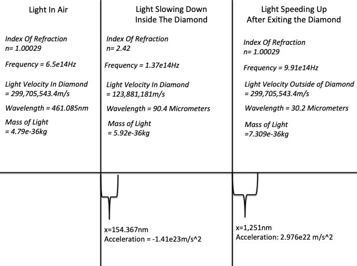
Fig. 15: Recap of the Data Analysis of the Incident Light Ray, The Light in Diamond, and the Light exiting the diamond.
89
An interesting application for this is the gravitational slingshot effect seen when Carl Sagan and his team sent the Voyager 1 spacecraft by Jupiter.
The following math shows why the culprit was time dilation itself.
We can add velocity with the gravity assist as follows:
GMm
r 2 ⋅ r = mar
GMm r = mar
GM
= ar
GM
r 2 = a
GM
r 2 = x t 2
M = t
GM 2
r 2 = x t a = v moving vstationary ( ) c
As the Mass of the planet gets larger, theirs a larger velocity addition, and consequent sharing of electric field energy. This decreases the time and creates a net acceleration of the spacecraft as seen on voyager 2.
90
v moving vstationary t = v moving vstationary ( ) c t stationary ( c 2 ( v moving ± vstationary ) 2
a =
r
t stationary ( c 2 ( GM 2 r 2 + vstationary ) 2
22.
CERN’S Compact Muon Solenoid and LIGO prove that the potential energy of all masses is distributed within linear precisions of time. And time is dimensionality itself.
In the LHC the collision increases the velocity due to the proton – proton collision. This creates more standing waves and increases the dimensionality, which increases the distribution of time in each dimension. For this reason, we see a zoo of particles coming out in the time dimensions.
We can account for all the dark energy in the universe with black hole, galactic, and stellar energetic analysis because the energy is uniformly distributed in the whole universe evenly in infinite radial time dimensions.
Dimensionality is defined by the time distribution itself.
If you notice in the picture below. The precision of collisions of two protons within a small confined space creates a linear time distribution in many dimensions that extend radially outwards. The mechanism for the distribution of energy in the time dimensions is too theoretically advanced to describe, but I will note, that due to the experimental evidence that I provided we can conclude that the energy is distributed in a time dimension as large as the universe itself.
91
d 2 = x 2 + y 2 + z 2 + t n 2 n =1 N ∑
Fig. 16: A proton – proton collision expands its energy in infinite time dimensions.
We can show mathematically, with the theory derived by Gauss and Ludwig Boltzmann, that the distribution of energy is distributed in an infinite Dimension of time.
My colleague Stephen Hawking and Minkowsky called this time imaginary. Einstein postulated that there was a change in curvature in space-time.
The following is the proof that the signal is infinite in extent (since the integral requires an infinite-dimensional existence to compute). The proof can be found in [27] http://hyperphysics.phy-astr.gsu.edu/hbase/Kinetic/molke.html#c1
Note that space has to be infinite for us to be able to compute the following integral. Because the universe is infinitely big!
This solution proves that the gravitational potential energy is stored in the infinite time dimension. f ( E ) = Ae E / kT
92
( v z
m 2π kT = e mv z 2 2 kT v z 2 = m 2π kT v z 2 ∞ ∞ ∫ e mv z 2 2 kT dv z x 2 ∞ ∞ ∫ e x 2 a dx = π 2 a 3/ 2 x = v z a = 2 kT m v z 2 = m 2π kT π 2 2 kT m ⎡ ⎣ ⎢ ⎤ ⎦ ⎥ 3/ 2 = kT m m 2 v z 2 = 3kT 2 = GmM r
f
) =
Another thing we can notice using the universal heat equation, is that time can flow in infinite directions and it can also be stopped. God Modulates time and I want to thank him for making this beautiful universe.
It makes sense that time has to be infinite. Because if it was not in the past, we wouldn’t be able to exist, because the negative infinity of time would never converge.
The following is a beautiful quote that describes the interplay between GOD, space, and time, and its relationship with all of existence.
The views of space and time which I wish to lay before you have sprung from the soil of experimental physics, and therein lies their strength. They are radical. Henceforth space by itself, and time by itself, are doomed to fade away into mere shadows, and only a kind of union of the two will preserve an independent reality.
Hermann Minkowski, 1908, 1909[7]
And thus these established relationships further prove our Grand Unified Theory of The Universe!
93
mc 2 = c 2 t 1/ 2 1 e 9 c 2 t + 1 e πc 2 t ⎛ ⎝ ⎜ ⎜ ⎞ ⎠ ⎟ ⎟ t = 1 t 1/ 2 1 e 9 c 2 t + 1 e πc 2 t ⎛ ⎝ ⎜ ⎜ ⎞ ⎠ ⎟ ⎟ t 3/ 2 = 1 e 9 c 2 t + 1 e πc 2 t ⎛ ⎝ ⎜ ⎜ ⎞ ⎠ ⎟ ⎟ t o = lim t → ±∞ t t o = lim t →0 t = 0
References:
1. Thomas Young. 1804 Experiments and Calculations Relative to Physical Optics
2. David Halliday, Robert Resnick, June 30, 2020, Fundamentals of Physics 6th edition,
3. E.A Hessels, et al, A measurement of the atomic hydrogen Lamb shift and the proton charge radius, DOI: 10.1126/science/aau7807. https://science.sciencemag.org/content/365/6457/1007
4. Charles Kittel, November 11th, 2004, Introduction to Solid State Physics.
5. Dr. Christine P Cheney, Photoelectric Effect Prelab, http://www.phys.utk.edu/labs/Photoelectric%20Effect%20Prelab.pdf
6. https://public.wsu.edu/~pchemlab/documents/Work-functionvalues.pdf
7. Albert Einstein, 1905, On a Heuristic point of view concerning the production and transformation of light.
8. https://www.baynews9.com/fl/tampa/weather/2020/10/06/the-dreaded-pinhole-eye
9. Mark Buchannan. August 2019 Light Seems to Pull Electrons Backward Physical Review Letters by Physics 12, 88
10. Jared H Strait et al. 2019 Revisiting the Photon-Drag Effect in Metal films Physical Review Letters DOI: 10.1103/PhysRevLett/123.053903
11. Dwyer 2003; 2007; 2012; Babich et al. 2005; Liu and Dwyer 2013; Skeltved et al. 2014 Positron Clouds within Thunderstorms
12. Dwyer, J. R. (2012), The relativistic feedback discharge model of terrestrial gamma ray flashes, J. Geophys. Res., 117, A02308, doi:10.1029/2011JA017160.
13. Logan W. Clark, Ningyuan Jia, Nathan Schine, Claire Baum, Alexandros Georgakopoulos & Jonatan Simon. 2019 Nature Interacting Floquet polaritons Nature 571, 532-536
14. M. J. Reid & T. M. Dame. On The Rotation Speed Of The Milky Way Determined from H1 Emission.
15. Charles Francis and Erik Anderson.Two estimates of the distance to the Galactic center
16. Eisenhauer, F.; et al. (July 20, 2005). SINFONI in the Galactic Center: Young Stars and Infrared Flares in the Central Light-Month. The Astrophysical Journal. 628 (1): 246–259
17. Wikipedia entry of Sagittarius A*. https://en.wikipedia.org/wiki/Sagittarius_A*
18. Stephen Hawking ,1966. Properties of expanding universes (Doctoral thesis)
19. A. Boehle, A. M. Ghez, R. Schödel, L. Meyer, S. Yelda, S. Albers, G. D. Martinez, E. E. Becklin, T. Do, J. R. Lu, K. Matthews, M. R. Morris, B. Sitarski, G. Witzel
94
(2016)“An Improved Distance and Mass Estimate for Sgr A* from a Multistar Orbit Analysis by A. Boehle et al.”
20. Gillessen et al., 2018, An Update on Monitoring Stellar Orbits in the Galactic Center Or Monitoring Stellar Orbits Around the Massive Black Hole in the Galactic Center
21. S.Gillessen et al., 2012, A gas cloud on its way toward the super-massive black hole in the Galactic Center”published.
22. Ru-Sen Lu et al. Detection of intrinsic source structure at ~3 Schwarzschild radii with Millimeter-VLBI observations of SAGITTARIUS A*”
23. Ophir Gottliev, 3/20/2007, Deriving the Heat Kernel in 1 Dimension
24. Matthew J. Hancock, 2006, Infinite Spatial Domains and the Fourier Transform
25. http://hyperphysics.phy-astr.gsu.edu/hbase/Kinetic/maxspe.html#c2
26. http://hyperphysics.phy-astr.gsu.edu/hbase/Waves/wavsol.html#c2
27. http://hyperphysics.phy-astr.gsu.edu/hbase/Kinetic/molke.html#c1
28. https://www.victorcanera.com/education/diamonds/light-performance
95