
Public Finance and Public Policy 5th Edition Gruber Solutions Manual Visit to Download in Full: https://testbankdeal.com/download/public-finance-and-publi c-policy-5th-edition-gruber-solutions-manual/

1. Assume that the price of a bus trip is $1, and the price of a gallon of gas is $2.50. What is the relative price of a gallon of gas, in terms of bus trips? What happens when the price of a bus trip rises to $1.25?
A commuter could exchange 2.5 bus trips for 1 gallon of gas (both will cost $2.50), so the relative price of a gallon of gas is 2.5 bus trips. At $1.25 per bus trip, the relative price of a gallon of gas has dropped to $2.50 ÷ $1.25 = 2 bus trips.
2. Draw the demand curve Q = 250 − 10P. Calculate the price elasticity of demand at prices of $5, $10, and $15 to show how it changes as you move along this linear demand curve.
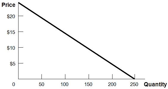
One way to sketch a linear demand function is to find the x (Q) and y (P) intercepts. Q = 0 when P = $25. When P = 0, Q = 250.
Solving for P = $5, Q = 250 − 10(5) = 250 − 50 = 200.
Similarly, solving for P = $10, Q = 250 10(10) = 150.
And solving for P = $15, Q = 250 − 150 = 100.
Price elasticity is the percent change in the quantity purchased divided by the percent change in price. To calculate these percentage changes, divide the change in each variable by its original value. Moving in $5 increments:
As P increases from $5 to $10, Q falls from 200 to 150. Therefore, P increases by 100% (5/5) as Q falls by 25% (50/200). Elasticity = 0.25/1.00 = 0.25.
As P increases from $10 to $15, Q falls from 150 to 100. P increases by 50% (5/10) as Q falls by 33% (50/150).
Elasticity = 0.33/0.5 = 0 66
As P increases from $15 to $20, Q falls from 100 to 50. P increases by 33% (5/15) and Q falls by 50% (50/100). Elasticity is 0.5/0.33 = 1.51.
Even though the magnitude of the change remains the same (for every $5 increase in price, the quantity purchased falls by 50), in terms of percentage change, the elasticity of demand increases in magnitude as price increases.
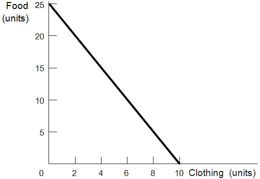
3. You have $100 to spend on food and clothing. The price of food is $ 4 and the price of clothing is $10.
a. Graph your budget constraint.
The food intercept (y in the accompanying figure) is 25 units. If you spend the entire $100 on food, at $4 per unit you can afford to purchase 100/4 = 25 units. Similarly, the clothing intercept (x) is 100/10 = 10. The slope, when food is graphed on the vertical axis, will be 2.5, which is equal (in absolute value) to the ratio of the price of clothing to the price of food (10/4).
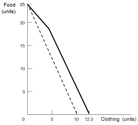
b. Suppose that the government subsidizes clothing such that each unit of clothing is half-price, up to the first 5 units of clothing. Graph your budget constraint in this circumstance.
This budget constraint will have two different slopes. At quantities of clothing less than or equal to 5, the slope will be 1.25 because the ratio of the price of clothing to the prices of food is now 5/4. In other words, for less than 5 units of clothing, 1 unit of clothing costs the same as 1.25 units of food, instead of 2.5 units of food. At quantities of clothing greater than 5, the slope will be 2.5 (if graphed with food on the y-axis), parallel to the budget constraint in shown in part a. The point where the line kinks, (5, 18.75), is now feasible because $5(5) + $4(18.75) = $100. The new x-intercept (clothing intercept) is 12.5: if you purchase 5 units at $5 per unit, you are left with $75 to spend. If you spend the rest of it on clothing at $10 per unit, you can purchase 7.5 units, for a total of 12.5 units.
New budget constraint (bold) and original (dashed):
The theory of diminishing marginal utility predicts that the more people eat the less utility they gain from each additional unit consumed. The marginal price of an additional unit of food at an all-you-can-eat buffet is zero; rational consumers will eat only until their marginal utility gain from an additional bite is exactly zero. The marginal cost of remaining at the buffet is the value of the time spent on the best alternative activity. When the marginal benefit of that activity is greater than the marginal benefit of remaining at the buffet, diners will leave.
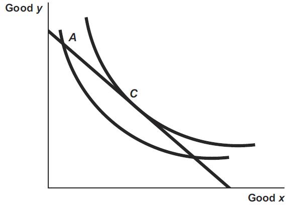
5. Explain why a consumer’s optimal choice is the point at which her budget constraint is tangent to an indifference curve.
Consumers optimize their choice when they are on the highest possible indifference curve given their budget constraint. Suppose a consumer’s choice is feasible (on the budget constraint) but not at a tangency, as at point A in the accompanying figure. Under these circumstances, the budget constraint must pass through the indifference curve where it intersects the chosen point. There must then be at least a segment of the budget constraint that lies above (up and to the right of) the indifference curve associated with that choice. Any choice on that segment would yield higher utility. Only when no part of the budget constraint lies above the indifference curve associated with a consumer’s choice are no feasible improvements in utility possible. The single tangency point (C in the figure) is the only point at which this occurs.
6. Consider the utilitarian social welfare function and the Rawlsian social welfare function, the two social welfare functions described in this chapter.
a. Which one is more consistent with a government that redistributes from rich to poor? Which is more consistent with a government that does not do any redistribution from rich to poor?
The Rawlsian social welfare function is consistent with redistribution from the rich to the poor whenever utility is increasing in wealth (or income). The utilitarian social welfare function can also be consistent with a government that redistributes from the rich to the poor, for example, if utility depends only on wealth and exhibits diminishing marginal utility. However, the Rawlsian social welfare function depends entirely on the least-well-off, so it will generally prescribe more redistribution than the utilitarian social welfare function.
b. Think about your answer to part a. Show that government redistribution from rich to poor can still be consistent with either of the two social welfare functions.
If utility depends only on wealth and exhibits diminishing marginal utility, and if efficiency losses from redistribution are small, then both the utilitarian and Rawlsian social welfare functions can be consistent with government redistribution. A simple example can illustrate this point. Suppose that utility as a function of wealth is expressed as v = √w, and that a rich person has wealth of $100 (yielding utility of 10) and a poor person has wealth of $25 (yielding utility of 5). The sum of utilities is 10 + 5 = 15.
Tax the wealthy person $19; their remaining wealth is $81, yielding utility of 9. Give $12 of the $19 to the poor person; this yields wealth of 25 + 12 = $37. The square root (utility) of 37 is greater than 6, so total utility is now greater than 15, even with the efficiency loss of $7 ($19 − $12). Under the Rawlsian function, which considers only the least-well-off person’s utility, social welfare has increased from 5 to greater than 6.
7. Because the free market (competitive) equilibrium maximizes social efficiency, why would the government ever intervene in an economy?
Efficiency is not the only goal of government policy. Equity concerns induce government to intervene to help people living in poverty, even when there are efficiency losses. In economic terms, a society that willingly redistributes resources has determined that it is willing to pay for or give up some efficiency in exchange for the benefit of living in a society that cares for those who have fewer resources. Social welfare functions that reflect this willingness to pay for equity or preference for equity may be maximized when the government intervenes to redistribute resources.
8. Consider an income guarantee program with an income guarantee of $ 5,000 and a benefit reduction rate of 40%. A person can work up to 2,000 hours per year at $10 per hour.
a. Draw the person’s budget constraint with the income guarantee.
A person will be ineligible for benefits if he or she earns $12,500 (guarantee of $5,000/40%) or more by working 12,500/10 = 1,250 or more hours (leaving 750 or fewer hours leisure)
b. Suppose that the income guarantee rises to $7,500 but with a 60% reduction rate. Draw the new budget constraint.
Benefits will end under these conditions when earned income is $7,500/0.60 = $12,500, just as shown in part a. The difference is that the all-leisure income is higher, but the slope of the line segment from 750 hours of leisure to 2,000 hours of leisure is flatter.
c. Which of these two income guarantee programs is more likely to discourage work? Explain.
A higher income guarantee with a higher reduction rate is more likely to discourage work for two reasons. First, not working at all yields a higher income. Second, a person who works less than 1,250 hours will be allowed to keep much less of his or her earned income when the effective tax rate is 60%. With a 60% benefit reduction rate, the effective hourly wage is only $4 per hour (40% of $10). In contrast, with a 40% benefit reduction rate, the effective hourly wage is $6 per hour (60% of $10).
d. Draw a system of smooth indifference curves that bend the right way but would lead an agent to work more under the program you chose in part c than under the other program. Describe what seems extreme about these curves that leads to the unusual behavior.
This is odd behavior. As part c indicated, the system from part b seems more likely to discourage work, as it has a lower effective wage ($4 vs $6). Moreover, as the graph indicates, the part b system makes the worker richer (leaving them with more money for any given amount of work less than 1,250 hours). One would typically expect that making someone richer would also discourage work by making earnings less pressing and encouraging extra leisure. But that’s not what’s happening here: the individual is working more (enjoying less leisure) under the system in part c.
Graphically, what’s going on is that the indifference curves are getting farther apart vertically as more leisure is consumed. Economically speaking, this is happening because these indifference curves imply that leisure is an inferior good for this individual. Giving this individual more money is making them consume less leisure (and therefore work more). And this inferior good effect is strong enough to outweigh the substitution effect coming from the lower effective wage in part c.
Such behavior is highly unlikely to happen in the real world.
9. A good is called normal if a person consumes more of it when her income rises (for example, she might see movies in theaters more often as her income rises). It is called inferior if a person consumes less of it when her income rises (for example, she might be less inclined to buy a used car as her income rises). Sally eats out at the local burger joint quite frequently. The burger joint suddenly lowers its prices.
a. Suppose that, in response to the lower burger prices, Sally goes to the local pizza restaurant less often. Can you tell from this whether or not pizza is an inferior good for Sally?
You cannot. Since Sally eats at the burger joint quite a bit, falling burger prices imply that she is richer. If this was the only effect, you could indeed conclude that pizza is an inferior good Sally gets richer and buys less pizza. But there is also a substitution effect here: the relative price of pizza has gone up. This leads her to substitute away from pizza. If the substitution effect is bigger than the income effect for Sally, then she could respond in this way, even if pizza is a normal good.
b. Suppose instead that, in response to the lower burger prices, Sally goes to the burger joint less often. Explain how this could happen in terms of the income and substitution effects by using the concepts of normal and/or inferior goods.
The substitution effect says that when the relative price of burgers falls, Sally should consume
more of them. Since she actually consumes less of them, the income effect must be working in the opposite direction, leading her to consume fewer burgers (and it must be stronger than the substitution effect). Since the fall of burger prices made Sally richer, burgers must be an inferior good for Sally. (Note: A good for which falling prices leads to reduced consumption is known as a Giffen good. Giffen goods are observed in reality very rarely, if at all.)
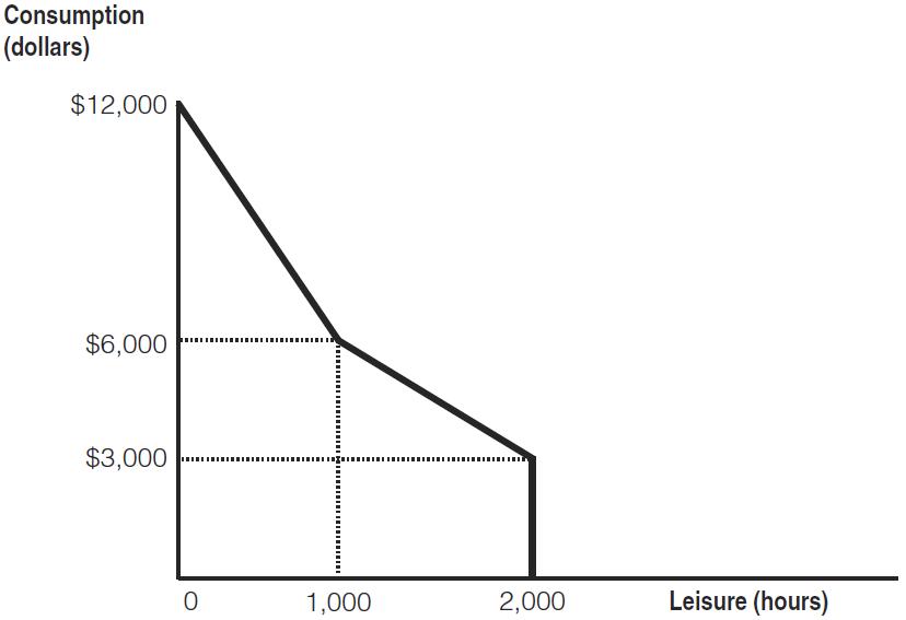
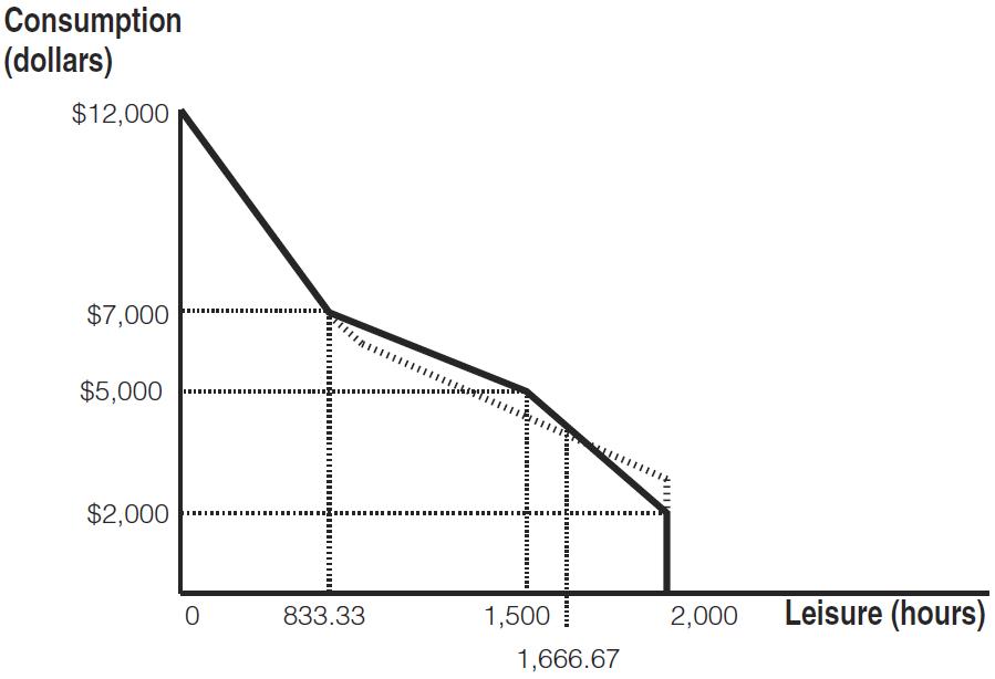
10. Consider an income guarantee program with an income guarantee of $3,000 and a benefit reduction rate of 50%. A person can work up to 2,000 hours per year at $6 per hour. Alice, Bob, Calvin, and Deborah work for 100, 333 ⅓, 400, and 600 hours, respectively, under this program. The government is considering altering the program to improve work incentives. Its proposal has two pieces. First, it will lower the guarantee to $2,000. Second, it will not reduce benefits for the first $3,000 earned by the workers. After this, it will reduce benefits at a reduction rate of 50%.
a. Draw the budget constraint facing any worker under the original program.
The budget constraint for the original program is depicted in the graph that follows. With zero hours worked (2,000 hours leisure), a worker gets to consume $3,000 the guaranteed income level. After earning 3000/0.50 = $6,000, which occurs at 6000/6 = 1,000 hours of work, the benefits have been reduced to zero.
b. Draw the budget constraint facing any worker under the proposed new program.
The budget constraint for the proposed program is depicted in the following graph. The original budget constraint is also depicted by the dashed line
At zero hours of work (2,000 hours of leisure), the worker now only gets to consume the lower $2,000 guarantee. She can work for up to 500 hours without any benefit reductions, so if she works for 500 hours, she gets to consume $5,000 (= $2,000 + $6/hr × 500 hrs) and has 1,500
hours of leisure.
After working an additional 2,000/3 ≈ 666.67 hours, for a total of about 1,133.33 hours of work or 833.33 hours of leisure, she will be receiving no benefits: her benefits have been reduced by 50% × $6/hr × 2,000/3 hrs = 50% × $4,000 = $2,000. At this point, she will be back onto the budget line that she would have been on, absent the guarantee program, just like under the old program.
c. Which of the four workers do you expect to work more under the new program? Who do you expect to work less? Are there any workers for whom you cannot tell if they will work more or less?
Workers working fewer than 500 hours see their hourly wage effectively doubled under the plan. The substitution effect therefore tends to make Alice, Bob, and Calvin all work more. One can calculate that the two budget constraints cross at 333 ⅓ hours of work, or 1,666.67 hours of leisure. The income effect is thus different for these three workers. Alice was working less than 333 ⅓ hours under the old policy, so the policy change effectively makes her poorer. She consumes less of all normal goods, including leisure, so this also makes her work more. We can unambiguously conclude that she will work more. Bob was working exactly 333 ⅓ hours, so he feels no income effect. We can conclude from the substitution effect alone that he too will work more. Calvin was working more than 333 ⅓ hours before, so this policy change effectively makes him richer. He will therefore tend to work less due to the income effect. We cannot tell if the substitution effect or the income effect is stronger, so we cannot tell if Calvin will work more or less. Finally, Deborah was working 600 hours before. Under both policies, the effective wage of someone working this many hours is $3/hr (since 50% of income is offset by reduced benefits). There is no substitution effect for her. As the graph shows, however, she experiences an increase in income. We conclude that she will work less.
11. Consider a free market with demand equal to Q = 900 − 10P and supply equal to Q = 20P.
a. What is the value of consumer surplus? What is the value of producer surplus?
The first step is to find the equilibrium price and quantity by setting quantity demanded equal to quantity supplied. Recall that the condition for equilibrium is that it is the price at which these quantities are equal.
From Q = 900 − 10P and Q = 20P, substitute: 900 − 10P = 20P. Adding 10P to each side of the equation yields 900 = 30P. Dividing both sides by 30 yields P = 30. If Q = 20P, then in equilibrium Q = 20(30) = 600.
Consumer and producer surplus are determined by finding the areas of triangles; area is equal to ½ the base times the height.
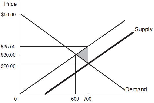

The vertical intercept of the demand curve is the price at which quantity demanded is zero: 0 = 900 − 10P. This solves to 90. The vertical intercept of the supply curve is zero, because 0 = 20P is solved by P = 0.
Consumer surplus = ½(600)(90 − 30) = ½(600)(60) = 18,000.
Producer surplus = ½(600)(30) = 9,000. Total surplus = 27,000.
b. Now the government imposes a $15 per unit subsidy on the production of the good. What is the consumer surplus now? The producer surplus? Why is there a deadweight loss associated with the subsidy, and what is the size of this loss?
A subsidy in effect lowers the cost of producing a good, yielding the bold supply line. The new supply function is Q = 20(P + 15) because the producer receives the price plus $15 when it produces. Solving for a new equilibrium,
20P + 300 = 900 − 10P 30P = 600.
P = $20; Q = 20 (20 + 15) = 700.
Consumer surplus = ½ (700)(90 − 20) = 24,500
Producer surplus = ½ (20 + 15)(700) = 12,250. Cost of subsidy = 15(700) = 10,500.
Total surplus = consumer surplus + producer surplus − cost of subsidy = 26,250, less than the original 27,000 There is efficiency loss because trades are induced for which the actual resource cost (without the subsidy) is greater than consumer willingness to pay. The deadweight loss is the area of the triangle that encompasses these new trades (the shaded area in the graph, pointing to the original equilibrium): ½ (700 − 600)(15) = 750
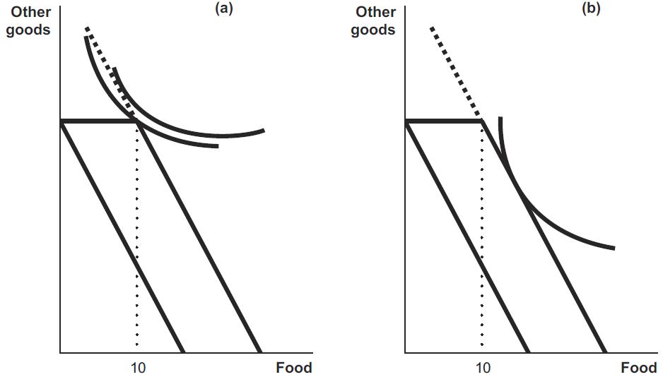
12. Governments offer both cash assistance and in -kind benefits, such as payments that must be spent on food or housing. Will recipients be indifferent between receiving cash versus in -kind benefits with the same monetary values? Use indifference curve analysis to show the circumstances in which individuals would be indifferent, and situations in which the form of the benefits would make a difference to them.
Generally recipients can attain a higher level of utility (they can choose a consumption bundle on a higher indifference curve) when they are given cash rather than a specific good. People who would purchase the same amount of food or housing as the in-kind grant provides would be indifferent between in-kind and cash benefits because they would use the cash to purchase the same items. However, people whose preferences would lead them to purchase less food or housing than the in-kind grant provides would prefer to receive cash. That way they could spend some of the cash on food or housing and the rest on the other goods they prefer. Suppose the government provides the first ten units of food at no cost. The person represented in panel (a) of the following graph would prefer cash. The indifference curve tangent to the extension of the new budget constraint identifies a consumption bundle that includes less than ten units of food. The person represented in panel (b) would choose the same point given cash or food. The optimal consumption bundle includes more than ten units of food.
13. Consider Bill and Ted, the two citizens in the country of Adventureland described in Problem 9 from Chapter 1. Suppose that Bill and Ted have the same utility function U (Y) = Y1/2 , where Y is
consumption (which is equal to net income).
a. Rank the three tax policies discussed in Problem 9 from Chapter 1 for a utilitarian social welfare function. Rank the three for a Rawlsian social welfare function.
The utility function is increasing in income. Rawlsian social welfare is therefore equal to the utility of the individual with lower income. For 0% and 25% tax rates, Ted has the lower incomes ($120 and $320, respectively). For a 40% tax rate, Bill has the lower income ($240). Since $320 > $240 > $120, Rawlsian social welfare is highest under the 25% tax rate and lowest under the 40% tax rate. To compute utilitarian social welfare, we compare:
Utilitarian social welfare with a 0% tax = 1,0001/2 + 1201/2 ≈ 42.58
Utilitarian social welfare with a 25% tax = 6001/2 + 3201/2 ≈ 42.38
Utilitarian social welfare with a 40% tax = 2401/2 + 2801/2 ≈ 32.22
We see that the 0% tax rate is best.
b. How would your answer change if the utility function was instead U (Y) = Y1/5? This change does not affect the order of tax rates according to the Rawlsian social welfare function. To compute social welfare for the utilitarian social welfare function we compare:
utilitarian social welfare with 0% tax = (1,000)1/5 + 1201/5 ≈ 6.59.
utilitarian social welfare with 25% tax = 6001/5 + 3201/5 ≈ 6.76.
utilitarian social welfare with 40% tax = 2401/5 + 2801/5 ≈ 6.08.
We see that the 25% tax rate is best and the 40% tax rate is the worst.
c. Suppose that Bill and Ted instead have different utility functions: Bill’s utility is given by UB(Y) = ¼Y1/2, and Ted’s is given by UT(Y) = Y1/2. (This might happen, for example, because Bill has significant disabilities and therefore needs more income to get the same level of utility.) How would a Rawlsian rank the three tax policies now?
Since the two have different utility functions, it is no longer easy to see who is better off under each situation. Under the 0% tax policy, we see that Ted has utility 1201/2 ≈ 10.95 and Bill has utility ¼ 1,0001/2 ≈ 7.91. We see that Bill is worse off under this policy. Since the other two tax policies make Bill worse off and Ted better off than the 0% policy, Bill’s utility will be used to compute Rawlsian social welfare. Rawlsian social welfare is highest with 0% taxes and lowest with 40% taxes, the policies that make Bill the best and worst off, respectively.
14. You have $4,000 to spend on entertainment this year (lucky you!). The price of a day trip (T ) is $40 and the price of a pizza and a movie ( M) is $20. Suppose that your utility function is U(T,M) =
T3/4M1/4 .
a. What combination of T and M will you choose?
This question can be solved by students who have taken calculus, following the approach described in the appendix to the chapter.
The constrained optimization problem can be written as Max T3/4M1/4 subject to $4,000 = 40T + 20M
Rewriting the budget constraint as M = 200 − 2T and substituting into the utility function gives Max T3/4(200 − 2T)1/4
Taking the derivative with respect to T and setting equal to zero gives 3/4T–1/4 (200 − 2T)1/4 − 1/2T3/4(200 − 2T)–3/4 = 0.
Rearranging gives (3/2)(200 − 2T) = T, or T = 75
Plugging back into the budget constraint gives M = 200 − 2(75) = 50.
You take 75 trips and go on 50 movie-and-a-pizza outings.
b. Suppose that the price of day trips rises to $50. How will this change your decision?
The new constrained optimization problem can be written as Max T3/4M1/4 subject to $4,000 = 50T + 20M
Rewriting the budget constraint as M = 200 − 2.5T and substituting into the utility function gives Max T3/4(200 − 2.5T)1/4
Taking the derivative with respect to T and setting equal to zero gives 1/3T–1/4 (200 − 2.5T)1/4 − 5/8T3/4(200 − 2.5T)–3/4 = 0.
Rearranging gives 6/5(200 − 2.5T) = T, or T = 60.
Plugging back into the budget constraint gives: M = 200 − 2.5(60) = 50.
You now take 60 trips and go on 50 movie-and-a-pizza outings.


2.1
2.2
Single Mothers
2.3 Equilibrium and Social Welfare
2.4 Welfare Implications of Benefit Reductions: The TANF Example Continued
2.5 Conclusion
Theoretical Tools of Public Finance 2 Heather
This chapter covers the theoretical tools of public finance.
• Theoretical tools: The set of tools designed to understand the mechanics behind economic decision making.
• Empirical tools: The set of tools designed to analyze data and answer questions raised by theoretical analysis.
We can illustrate how consumers are presumed to make choices in four steps:
1.First, we discuss how to model preferences graphically.
2.Then, we show how to take this graphical model of preferences and represent it mathematically with a utility function.
3.Next, we model the budget constraints that individuals face.
4.Finally, we show how individuals maximize their utility (make themselves as well off as possible) given their budget constraints.
• Utility function: A mathematical function representing an individual’s set of preferences, which translates her well-being from different consumption bundles into units that can be compared in order to determine choice.
• Constrained utility maximization: The process of maximizing the well-being (utility) of an individual, subject to her resources (budget constraint).
• Models: Mathematical or graphical representations of reality.
• Indifference curve: A graphical representation of all bundles of goods that make an individual equally well off. Because these bundles have equal utility, an individual is indifferent as to which bundle he consumes.
• Indifference curves have two key properties:
1.Consumerspreferhigherindifferencecurves.
2.Indifferencecurvesarealwaysdownwardsloping.
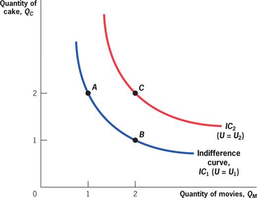
• Consumer is indifferent between A and B.
• C is preferred to A or B.

• Consumer is indifferent between A and B.
• C is preferred to A or B.
• Underlying the indifference curves is an individual’s utility function.
• A utility function is some mathematical representation,
• and so on are the quantities of the goods consumed.
• is some mathematical function that describes how consumption of each good translates to utility.
• Example utility function: Andrea’s utility for CDs ( ) and Movies ( ) is:
• Andrea is indifferent between 4 CDs and 1 movie, or 1 CD and 4movies.
• Andrea prefers 3 CDs and 3movies to either bundle.
How much do consumers like a good?
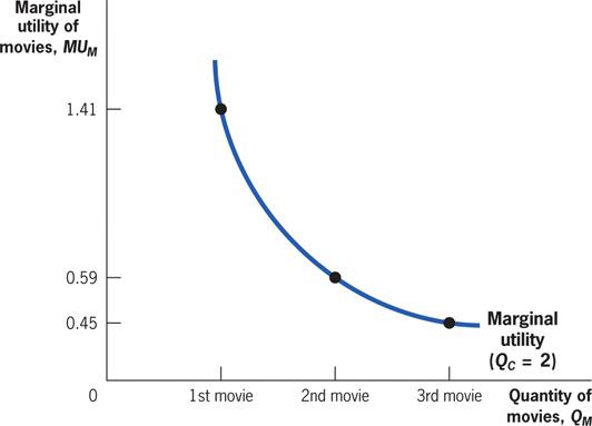
• Marginal utility: The additional increment to utility obtained by consuming an additional unit of a good.
•
Diminishing marginal utility: The consumption of each additional unit of a good makes the individual less happy than the consumption of the previous one.
• Many utility functions exhibit diminish marginal utility, including
o The first bite of pizza is often the tastiest.
With each additional movie consumed, utility increases but by ever smaller amounts.
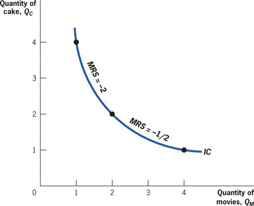
• Marginal rate of substitution (MRS): The rate at which a consumer is willing to trade one good for another.
• Moving along an indifference curve keeps a consumer equally well off, so
• The MRS is equal to the slope of the indifference curve, the rate at which the consumer will trade the good on the vertical axis for the good on the horizontal axis.
As Andrea moves down the indifference curve, getting more movies and fewer cakes, the marginal utility of cakes rises, and the marginal utility of movies falls, lowering the MRS.
• Budget constraint: A mathematical representation of all the combinations of goods an individual can afford to buy if she spends her entire income.
• Opportunity cost: The cost of any purchase is the next best alternative use of that money, or the forgone opportunity.
• Quick hint: When a person’s budget is fixed, if he buys one thing he is, by definition, reducing the money he has to spend on other things. Indirectly, this purchase has the same effect as a direct good-for-good trade.
The slope of the budget constraint is the rate at which she can trade cakes for movies in the marketplace, PM/PC = –8⁄16 = –1⁄2.
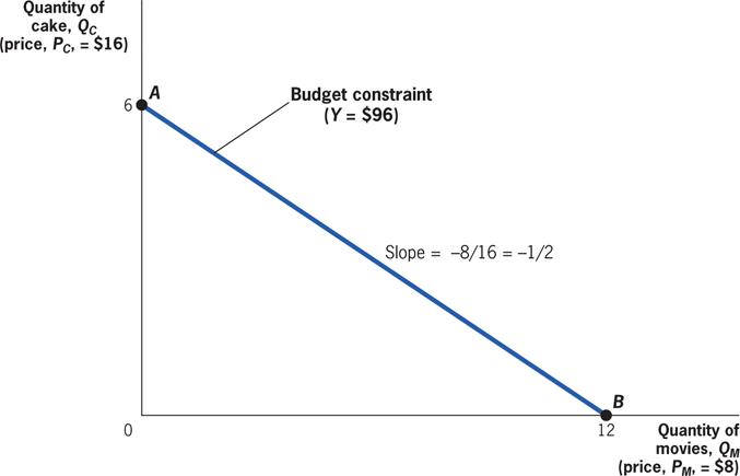
• The slope of the budget constraint says how much of one good you can buy if you give up one unit of the other, .
• The marginal rate of substitution says how much you like trading one good for another.
• If � � , you get more utility buying fewer CDs and more movies.
• If � � , you get more utility buying more CDs and fewer movies.
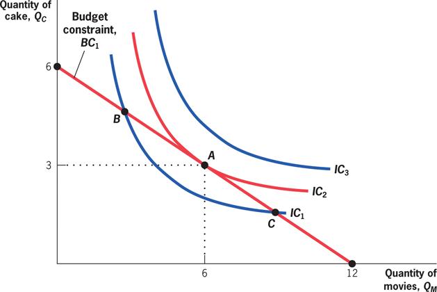
• To maximize utility, therefore:
• Or, find tangency between indifference curves and budget constraint.
Whenever a consumer is at a point where the indifference curve and the budget constraint are not tangent, she can make herself better off by moving to a point of tangency.
• Maximizing utility tells us how many goods a person buys at a given price.
• What happens when we change the prices?
• Substitution effect: Holding utility constant, a relative rise in the price of a good will always cause an individual to choose less of that good.
• Income effect: A rise in the price of a good will typically cause an individual to choose less of all goods because her income can purchase less than before.
The substitution effect holds utility constant but changes the income while reflecting the change in relative prices.

How do changes in income affect demand?
• Normal goods: Goods for which demand increases as income rises.
• Inferior goods: Goods for which demand falls as income rises.
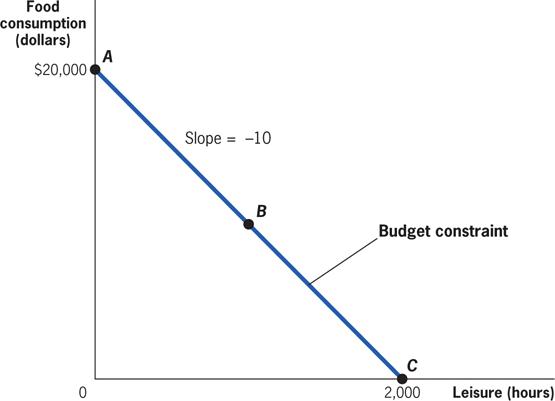
The TANF program was created in 1996 and provides a monthly support check to families with incomes below a threshold level that is set by each state.
• Suppose that Joelle is a single mother who spends all of her earnings and TANF benefits on food for herself and her children.
• By working more hours, she can earn more money for food, but she has less time at home with her children and for leisure.
• She would prefer time at home to time at work (leisure is a normal good). With these preferences, more work makes Joelle worse off, but it allows her to buy more food.
• How does Joelle decide on the optimal amount of labor to supply?
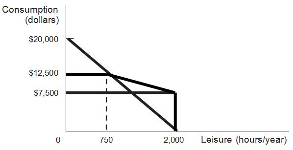
If she takes no leisure, she can have consumption of $20,000 per year; but if she takes 2,000 hours of leisure, her consumption falls to 0. This is represented by the budget constraint with a slope of –10, the relative price of leisure in terms of food consumption.
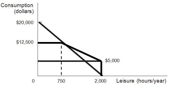
Point D marks the end of the new budget constraint and provides a new option: she can have 2,000 hours of leisure and $5,000 in food consumption because of the $5,000 TANF benefit guarantee.
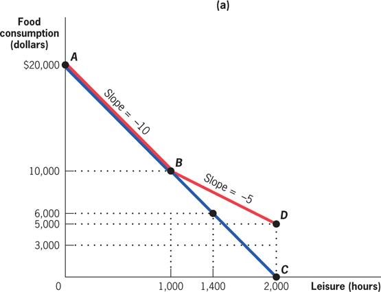
If the guarantee falls to $3,000, the budget constraint (AEF) doesn’t flatten until she takes more than 1,400 hours of leisure; now, with 2,000 hours of leisure, her consumption is only $3,000 at point F.
The substitution effect holds utility constant but changes relative prices.
The size of the response depends on:
• How much was earned before the benefit change.
• The size of the income and substitution effects on her leisure/labor decision.
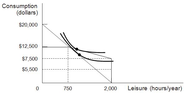
• Let’s consider two individuals: Individual 2 values leisure more highly relative to consumption than Individual 1 does.
When the TANF guarantee is $5,000, the optimal choice is to take 1,910 hours of leisure and consume $5,450 (at point A). When the guarantee falls to $3,000, she reduces her leisure to 1,655 hours, and her consumption falls to $4,725 (at point B).
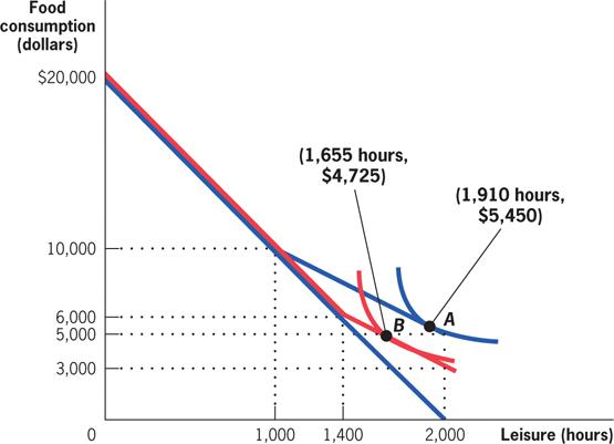
Because leisure is valued more highly relative to consumption for this individual, she chooses 2,000 hours of leisure regardless of the TANF guarantee. The reduction in guarantee therefore lowers her consumption from $5,000 (at point A) to $3,000 (at point B).
How do markets determine what gets produced? Do they produce the right amount?
• Market: The arena in which demanders and suppliers interact.
• Market equilibrium: The combination of price and quantity that satisfies both demand and supply, determined by the interaction of the supply and demand curves.
• Welfare economics: The study of the determinants of well-being, or welfare, in society.
How much of a good do people want to buy at the market price?
• Demand curve: A curve showing the quantity of a good demanded by individuals at each price.
• Obtained by finding the utility-maximizing bundle at each price.