Full link downoad Calculus Single and Multivariable 6th
Edition by Hughes-Hallett Gleason and McCallumTest bank:
https://testbankpack.com/p/test-bank-for-calculus-single-andmultivariable-6th-edition-by-hughes-hallett-gleason-and-mccallum-isbn047088861x-9780470888612/
Solution manual:
https://testbankpack.com/p/solution-manual-for-calculussingle-and-multivariable-6th-edition-by-hughes-hallett-gleasonand-mccallum-isbn-047088861x-9780470888612/
CHAPTER TWO
Solutions for Section 2.1
2. The average velocity over a time period is the change in position divided by the change in time. Since the function x(t) gives the position of the particle, we find the values of x(0) = 2 and x(4) = 6 Using these values, we find
3. The average velocity over a time period is the change in position divided by the change in time Since the function x(t) gives the position of the particle, we find the values of x(2) = 14 and x(8) = 4 Using these values, we find
4. The average velocity over a time period is the change in position divided by the change in time. Since the function s(t) gives the distance of the particle from a point, we read off the graph that s(0) = 1 and s(3) = 4 Thus,
5. The average velocity over a time period is the change in position divided by the change in time Since the function s(t) gives the distance of the particle from a point, we read off the graph that s(1) = 2 and s(3) = 6. Thus,
6. The average velocity over a time period is the change in position divided by the change in time. Since the function s(t) gives the distance of the particle from a point, we find the values of s(2)
Using these values, we find
7. Theaverage velocity overa timeperiod is the change in the distance divided by thechange in time.Sincethefunction s(t) √ √ gives the distance of the particle from a point, we find the values of s(π/3) = 4 + 3 3/2 and s(7π/3) = 4 + 3 3/2 Using these values, we find
Though the particle moves, its average velocity is zero, since it is at the same position at
8. (a) Let s = f (t).
(i) We wish to find the average velocity between t = 1 and t = 1 1 We have
(ii)
(b) We see in part (a) that as we choose a smaller and smaller interval around t = 1 the average velocity appears to be getting closer and closer to 6, so we estimate the instantaneous velocity at t = 1 to be 6 m/sec
9. (a) Let s = f (t).
(i) We wish to find the average velocity between t = 0 and t = 0 1 We have
(b) We see in part (a) that as we choose a smaller and smaller interval around t = 0 the average velocity appears to be getting closer and closer to 0, so we estimate the instantaneous velocity at t = 0 to be 0 m/sec
Looking at a graph of s = f (t) we see that a line tangent to the graph at t = 0 is horizontal, confirming our result.
10 (a) Let s = f (t).
(i) We wish to find the average velocity between t = 1 and t = 1 1 We have
(ii) We have
(iii) We have
(b) We see in part (a) that as we choose a smaller and smaller interval around t = 1 the average velocity appears to be getting closer and closer to 0 83, so we estimate the instantaneous velocity at t = 1 to be −0 83 m/sec In this case, more estimates with smaller values of h would be very helpful in making a better estimate.
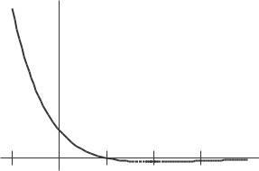
11. See Figure 2 1
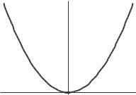
12 See Figure 2 2
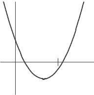
13 See Figure 2 3
Problems
14. Using h = 0 1, 0 01, 0 001, we see

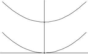
These calculations suggest that lim
15. Using radians,
These values suggest that lim
16. Using h = 0 1, 0 01, 0 001, we see
This suggests that lim 7 1 ≈ 1.9.

17. Using h = 0 1, 0 01, 0 001, we see
These values suggest that lim
fact, this limit is
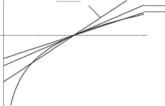
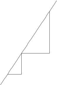
20. 0 < slope at C < slope at B < slope of AB < 1 < slope at A (Note that the line y = x, has slope 1.)
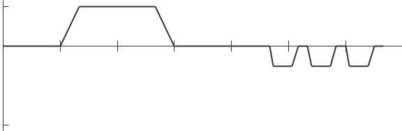
F <B <E <0<D <A<C. 22. ! Average velocity = s(0 2) s(0) 0 < t < 0.2 0.2− 0 ! Average velocity = s(0 4)− s(0 2) 0.2 < t < 0.4 0.4− 0.2 0.5 = 0.2 = 2.5 ft/sec 1.3 = 0.2 = 6.5 ft/sec
A reasonable estimate of the velocity at t = 0.2 is the average:
4
(b) After 1 second, the ball’s height is f (1) = 16 + 50 + 36 = 70 feet, so it traveled 70 36 = 34 feet in 1 second, and its average velocity was 34 ft/sec
(c) At t = 1.001, the ball’s height is f (1.001) = 70.017984 feet, and its velocity about 70 017984−70 = 17.984 18 ft/sec
(d) We complete the square:
f (t) = 16t 2 + 50t + 36
= 16 t 2 − 25 t + 36
2 25 625 625
= 16 t 8 t + 256 +36+16 256
= 16(t − 25 )2 + 1201 16
so the graph of f is a downward parabola with vertex at the point (25/16, 1201/16) = (1 6, 75 1). We see from Figure 2.5 that the ball reaches a maximum height of about 75 feet. The velocity of the ball is zero when it is at the peak, since the tangent is horizontal there
(e) The ball reaches its maximum height when t = 25 = 1.6.
Strengthen Your Understanding
29. Speed is the magnitude of velocity, so it is always positive or zero; velocity has both magnitude and direction
30. We expand and simplify first
Many other answers are possible.
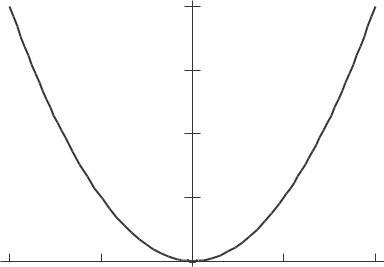
33. One possibility is the position function s(t) = t2 Any function that is symmetric about the line t = 0 works. For s(t) = t2 , the slope of a tangent line (representing the velocity) is negative at t = 1 and positive at t = 1, and that the magnitude of the slopes (the speeds) are the same.
34. False. For example, the car could slow down or even stop at one minute after 2 pm, and then speed back up to 60 mph at one minute before 3 pm. In this case the car would travel only a few miles during the hour, much less than 50 miles.
10 Chapter Two /SOLUTIONS
2.1 SOLUTIONS
35 False Its average velocity for the time between 2 pm and 4 pm is 40 mph, but the car could change its speed a lot during that time period For example, the car might be motionless for an hour then go 80 mph for the second hour. In that case the velocity at 2 pm would be 0 mph
36. True During a short enough time interval the car can not change its velocity very much, and so it velocity will be nearly constant. It will be nearly equal to the average velocity over the interval.
37. True The instantaneous velocity is a limit of the average velocities The limit of a constant equals that constant
38. True. By definition, Average velocity = Distance traveled/Time.
39. False Instantaneous velocity equals a limit of difference quotients.
Solutions for Section 2.2
Exercises
1. The derivative, f ′ (2), is the rate of change of x 3 at x = 2 Notice that each time x changes by 0 001 in the table, the value of x 3 changes by 0 012 Therefore, we estimate
f ′ (2) =Rate of change 0.012 of f at x = 2 ≈ 0.001 = 12
The function values in the table look exactly linear because they have been rounded For example, the exact value of x 3 when x = 2 001 is 8 012006001, not 8 012 Thus, the table can tell us only that the derivative is approximately 12. Example 5 on page 95 shows how to compute the derivative of f (x) exactly.
2. With h = 0 01 and h = 0 01, we have the difference quotients
= 0 001 and h = −0 001,
The values of these difference quotients suggest that the limit is about 3 0 We say
3. (a) Using the formula for the average rate of change gives
1 ≤ q ≤ 2
for 2 ≤ q ≤ 3 1
So we see that the average rate decreases as the quantity sold in kilograms increases.
(b) With h = 0.01 and h = 0.01, we have the difference quotients
R(2 01) R(2) = 59 9 dollars/kg and R(1 99) R(2) = 60 1 dollars/kg 0 01 0 01
With h = 0 001 and h = −0 001,
R(2 001) − R(2) = 59 99 dollars/kg and R(1 999) R(2) = 60 01 dollars/kg 0 001 0 001
The values of these difference quotients suggest that the instantaneous rate of change is about 60 dollars/kg To confirm that the value is exactly 60, that is, that R ′ (2) = 60, we would need to take the limit as h → 0.
First we find the average rates of change of f (x) = log x between x = 1.5 and x = 2, and between x = 2 and
Now we approximate the instantaneous rate of change at x = 2 by finding the average of the above rates, i e
Since sin x is decreasing for values near x = 3π, its derivative at x = 3π is negative
8 f ′ (1) = lim log(1 + h) − log 1 = lim log(1 + h)
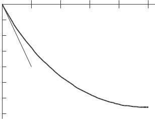
Evaluating log(1+h) for h = 0 01, 0 001, and 0 0001, we get 0 43214, 0 43408, 0 43427, so f ′ (1) ≈ 0 43427 The corresponding secant lines are getting steeper, because the graph of log x is concave down. We thus expect the limit to be more than 0 43427 If we consider negative values of h, the estimates are too large We can also see this from the graph below:
9. We estimate f ′ (2) using the average rate of change formula on a small interval around 2. We use the interval x = 2 to x = 2 001 (Any small interval around 2 gives a reasonable answer ) We have
001 2 = 2 001 2 = 0 001 = 9 89
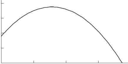
10. (a) The average rate of change from x = a to x = b is the slope of the line between the points on the curve with x = a and x = b Since the curve is concave down, the line from x = 1 to x = 3 has a greater slope than the line from x = 3 to x = 5, and so the average rate of change between x = 1 and x = 3 is greater than that between x = 3 and x = 5

(b) Since f is increasing, f (5) is the greater.
(c) As in part (a), f is concave down and f ′ is decreasing throughout so f ′ (1) is the greater.
11. Since f ′ (x) = 0 where the graph is horizontal, f ′ (x) = 0 at x = d The derivative is positive at points b and c, but the graph is steeper at x = c Thus f ′ (x) = 0.5 at x = b and f ′ (x) = 2 at x = c Finally, the derivative is negative at points a and e but the graph is steeper at x = e. Thus, f ′ (x) = 0.5 at x = a and f ′ (x) = 2 at x = e. See Table 2.3. Thus, we have f ′ (d) = 0, f ′ (b) = 0 5, f ′ (c) = 2, f ′ (a) = 0 5, f ′ (e) = 2.
Table 2.3
x f ′ (x) d
12. One possible choice of points is shown below
Problems
13. The statements f (100) = 35 and f ′ (100) = 3 tell us that at x = 100, the value of the function is 35 and the function is increasing at a rate of 3 units for a unit increase in x Since we increase x by 2 units in going from 100 to 102, the value of the function goes up by approximately 2 3 = 6 units, so
f (102) ≈ 35 + 2 3 = 35 + 6 = 41
14 The answers to parts (a)–(d) are shown in Figure 2 6
Slope= f ′ (3)
❄
✻✻✛ f (4) f (2)
f (x)
Slope= f (5)−f (2)
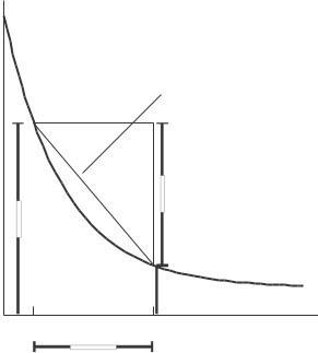
15. (a) Since f is increasing, f (4) > f (3).
(b) From Figure 2 7, it appears that f (2) − f (1) > f (3) − f (2).
(c) The quantity f (2) f (1) represents the slope of the secant line connecting the points on the graph at x = 1 2 1

(d)
and x = 2 This is greater than the slope of the secant line connecting the points at x = 1 and x = 3 which is f (3) f (1) 3 − 1
The function is steeper at x = 1 than at x = 4 so f ′ (1) > f ′ (4).
The quantities f ′ (2), f ′ (3) and f (3) − f (2) have the following interpretations:
• f ′ (2) = slope of the tangent line at x = 2
• f ′ (3) = slope of the tangent line at x = 3
• f (3) − f (2) = f (3) f (2) = slope of the secant line from f (2) to f (3). 3−2
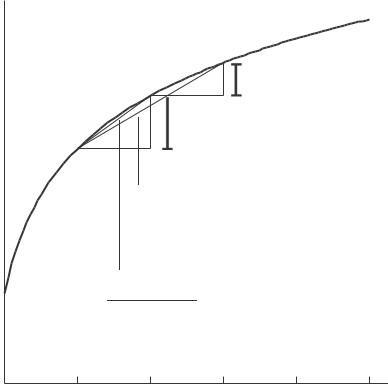
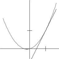
From Figure 2 8, it is clear that 0 < f (3) − f (2) < f ′ (2). By extending the secant line past the point (3, f (3)), we can see that it lies above the tangent line at x = 3 Thus 0 < f ′ (3) < f (3) − f (2) < f ′ (2).
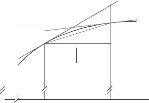
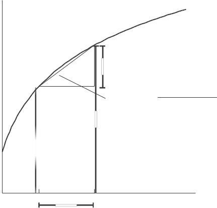
17 The coordinates of A are (4, 25) See Figure 2 9 The coordinates of B and C are obtained using the slope of the tangent line Since f ′ (4) = 1 5, the slope is 1.5
From A to B, ∆x = 0 2, so ∆y = 1 5(0 2) = 0 3 Thus, at C we have y = 25 + 0.3 = 25 3 The coordinates of B are (4 2, 25 3).
From A to C , ∆x = 0 1, so ∆y = 1 5(−0 1) = 0 15 Thus, at C we have y = 25 − 0 15 = 24 85 The coordinates of C are (3 9, 24 85).
18 (a) Since the point B = (2, 5) is on the graph of g, we have g(2) = 5 (b) The slope of the tangent line touching the graph at x = 2 is given by
20. See Figure 2 11
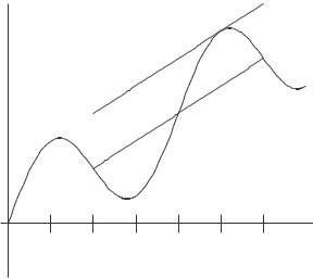
21 (a) For the line from A to B, Slope = f (b) f (a) b − a
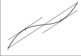
(b) The tangent line at point C appears to be parallel to the line from A to B. Assuming this to be the case, the lines have the same slope
(c) There is only one other point, labeled D in Figure 2 12, at which the tangent line is parallel to the line joining A and B.
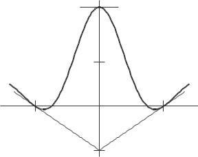
22. (a) Figure 2 13 shows the graph of an even function We see that since f is symmetric about the y-axis, the tangent line at x = 10 is just the tangent line at x = 10 flipped about the y-axis, so the slope of one tangent is the negative of that of the other. Therefore, f ′ ( 10) = f ′ (10) = 6.
(b) From part (a) we can see that if f is even, then for any x, we have f ′ (−x) = f ′ (x). Thus f ′ ( 0) = f ′ (0), so f ′ (0) = 0
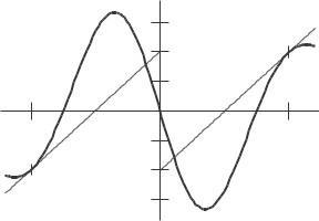
23 Figure 2 14 shows the graph of an odd function We see that since g is symmetric about the origin, its tangent line at x = 4 is just the tangent line at x = 4 flipped about the origin, so they have the same slope Thus, g ′ (−4) = 5
To four decimal places,
(b) Consider the ratio sin h h . As we approach 0, the numerator, sin h, will be much smaller in magnitude if h is in degrees than it would be if h were in radians. For example, if h = 1 ◦ radian, sin h = 0 8415, but if h = 1 degree, sin h = 0 01745 Thus, since the numerator is smaller for h measured in degrees while the denominator is the same, we expect the ratio sin h to be smaller h
25. We find the derivative using a difference quotient:
Thus at x = 3, the slope of the tangent line is
therefore its equation is
The graph is in Figure 2 15
26 Using a difference quotient with h = 0 001, say, we find
The fact that f ′ is larger at x = 2 than at x = 1 suggests that f is concave up between x
27 We want f ′ (2). The exact answer is f (2 + h) − f (2) (2 + h) 2+h 4
= lim = lim , h→0 h but we can approximate this. If h = 0 001, then h
h and if h = 0 0001 then
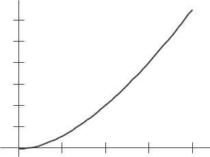
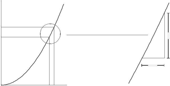
28. Notice that we can’t get all the information we want just from the graph of f for 0 ≤ x ≤ 2, shown on the left in Figure 2 16 Looking at this graph, it looks as if the slope at x = 0 is 0 But if we zoom in on the graph near x = 0, we get the graph of f for 0 ≤ x ≤ 0 05, shown on the right in Figure 2 16 We see that f does dip down quite a bit between x = 0 and x ≈ 0 11 In fact, it now looks like f ′ (0) is around 1 Note that since f (x) is undefined for x < 0, this derivative only makes sense as we approach zero from the right.
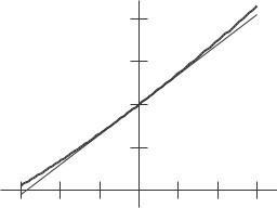
We zoom in on the graph of f near x = 1 to get a more accurate picture from which to estimate f ′ (1). A graph of f for 0.7 ≤ x ≤ 1.3 is shown in Figure 2 17 [Keep in mind that the axes shown in this graph don’t cross at the origin!] Here we see that f ′ (1) ≈ 3 5
′ (1) = lim f (1 + h) f (1) = lim ln(cos(1 + h)) ln(cos 1)
For h = 0.001, the difference quotient = 1.55912; for h = 0.0001, the difference quotient = −1.55758. The instantaneous rate of change of f therefore appears to be about 1.558 at x = 1. At
= π 4 , if we try h = 0 0001, then
The instantaneous rate of change of f appears to be about 1 at x = π 4
30. The quantity f (0) represents the population on October 17, 2006, so f (0) = 300 million The quantity f ′ (0) represents the rate of change of the population (in millions per year). Since 1 person
seconds
so we have f ′ (0) = 2.867.
6 mi = llion people = 2 867 million people/year,
60 24 365) years
31. We want to approximate P ′ (0) and P ′ (7). Since for small h
32 (a) From Figure 2 18, it appears that the slopes of the tangent lines to the two graphs are the same at each x For x = 0, the slopes of the tangents to the graphs of f (x) and g(x) at 0 are
= 2, the slopes of the tangents to the graphs of f (x) and g(x) are
+
+ C (f (x) + C ) h
lim f (x + h) f (x)
33. As h gets smaller, round-off error becomes important When h = 10−12 , the quantity 2h 1 is so close to 0 that the calculator rounds off the difference to 0, making the difference quotient 0 The same thing will happen when h = 10 20
34. (a) Table 2.4 shows that near x = 1, every time the value of x increases by 0.001, the value of x 2 increases by approximately 0 002 This suggests that f ′ (1) 0 002 = 2 0 001
(b) The derivative is the limit of the difference quotient, so we look at
f ′ (1)= lim f (1 + h) f (1) h→0 h
Using the formula for f , we have
Since the limit only examines values of h close to, but not equal to zero, we can cancel h in the expression (2h + h2 )/h We get
f ′ (1) = lim h(2 + h) h→0 h = lim (2 + h). h→0
This limit is 2, so f ′ (1) = 2 At x = 1 the rate of change of x 2 is 2
(c) Since the derivative is the rate of change, f ′ (1) = 2 means that for small changes in x near x = 1, the change in f (x) = x 2 is about twice as big as the change in x As an example, if x changes from 1 to 1 1, a net change of 0 1, then f (x) changes by about 0 2 Figure 2 19 shows this geometrically Near x = 1 the function is approximately linear with slope of 2
41. Using the definition of the derivative, we have
42. Usingthedefinition of the derivative, we have
which
43. Using the definition
47. As we saw in the answer to Problem 41, the slope of the tangent line to f (x) = 5x2 at x = 10 is 100 When x = 10, f (x) = 500 so (10, 500) is a point on the tangent line Thus y = 100(x − 10) + 500 = 100x − 500
48. As we saw in the answer to Problem 42, the slope of the tangent line to f (x) = x 3 at x = 2 is 12 When x = 2, f (x) = 8 so we know the point ( 2, 8) is on the tangent line Thus the equation of the tangent line is y = 12(x + 2) − 8 = 12x + 16
49 We know that the slope of the tangent line to f (x) = x when x = 20 is 1 When x = 20, f (x) = 20 so (20, 20) is on the tangent line Thus the equation of the tangent line is y = 1(x − 20) + 20 = x
50. First find the derivative of f (x) = 1/x2 at x = 1
= lim
Thus the tangent line has a slope of 2 and goes through the point (1, 1), and so its equation is
Strengthen Your Understanding
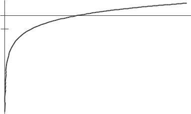
51 The graph of f (x) = log x is increasing, so f ′ (0 5) > 0
52. The derivative of a function at a point is the slope of the tangent line, not the tangent line itself
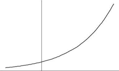
53. f (x) = e x
Many other answers are possible.
54 A linear function is of the form f (x) = ax + b The derivative of this function is the slope of the line y = ax + b, so f ′ (x) = a, so a = 2 One such function is f (x) = 2x + 1
55. True. The derivative of a function is the limit of difference quotients. A few difference quotients can be computed from the table, but the limit can not be computed from the table.
56.True The derivative f ′ (10) is the slope of the tangent line to the graph of y = f (x) at the point where x = 10 When you zoom in on y = f (x) close enough it is not possible to see the difference between the tangent line and the graph of f on the calculator screen. Thelineyouseeon the calculator is a littlepieceof thetangent line,so its slopeis the derivativef ′ (10).
57.True This is seen graphically The derivative f ′ (a) is the slope of the line tangent to the graph of f at the point P where x = a The difference quotient (f (b) − f (a))/(b − a) is the slope of the secant line with endpoints on the graph of f at the points where x = a and x = b The tangent and secant lines cross at the point P The secant line goes above the tangent line for x > a because f is concave up, and so the secant line has higher slope
58. (a). This is best observed graphically
Solutions for Section 2.3
Exercises
1 (a) We use the interval to the right of x = 2 to estimate the derivative. (Alternately, we could use the interval to the left of 2, or we could use both and average the results.) We have
f
(2)
f (4)− f (2) 24− 18 6
(b) We know that f ′ (x) is positive when f (x) is increasing and negative when f (x) is decreasing, so it appears that
2 For x = 0, 5, 10, and 15, we use the interval to the right to estimate the derivative For x = 20, we use the interval to the left. For x = 0, we have
Similarly, we find the other estimates in Table 2 5
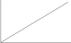
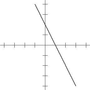
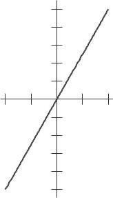
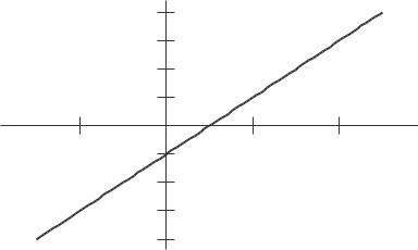
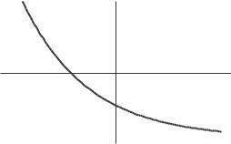
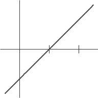
3 The graph is that of the line y = 2x + 2 The slope, and hence the derivative, is 2 See Figure 2 20
6. See Figure 2 23
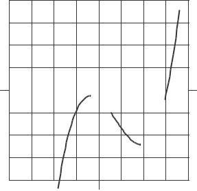
7. The slope of this curve is approximately 1 at x = 4 and at x = 4, approximately 0 at x = 2.5 and x = 1 5, and approximately 1 at x = 0 See Figure 2 24


14. See Figures 2 32 and 2 33
15. See Figures 2 34 and 2 35
16. The graph of f (x) and its derivative look the same, as in Figures 2.36 and 2.37.

17. See Figures 2 38 and 2 39
18 See Figures 2 40 and 2 41
19 Since 1/x = x 1 , using the power rule gives
20. Since
22.
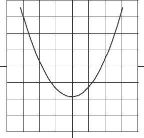
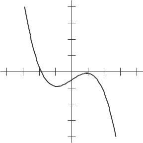
24. Since f ′ (x) > 0 for x < 1, f (x) is increasing on this interval. Since f ′ (x) < 0 for x > 1, f (x) is decreasing on this interval. Since f ′ (x) = 0 at x = 1, the tangent to f (x) is horizontal at x = 1. One possible shape for y = f (x) is shown in Figure 2.42.
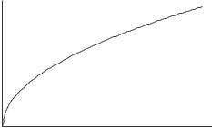
At x = 1, the values of ln x are increasing by 0 001 for each increase in x of 0 001, so the derivative appears to be 1 At x = 2, the increase is 0 0005 for each increase of 0 001, so the derivative appears to be 0 5 At x = 5, ln x increases by 0 0002 for each increase of 0 001 in x, so the derivative appears to be 0 2 And at x = 10, the increase is 0 0001 over intervals of 0 001, so the derivative appears to be 0 1 These values suggest an inverse relationship between x and f ′ (x), namely f ′ (x) = 1 x
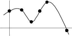
26. We know that f ′ (x) ≈ f (x + h) f (x) For this problem, we’ll take the average of the values obtained for h = 1 h
f (x + 1) − f (x − 1) and h = 1; that’s the average of f (x + 1) − f (x) and f (x) − f (x − 1) which equals
f ′ (0) ≈ f (1) − f (0) = 13 18 = 5.
f ′ (1) ≈ (f (2) − f (0))/2 = (10 − 18)/2 = 4.
f ′ (2) ≈ (f (3) − f (1))/2 = (9 13)/2 = −2. f ′ (3) ≈ (f (4) − f (2))/2 = (9 − 10)/2 = 0 5 f ′ (4) ≈ (f (5) − f (3))/2 = (11 9)/2 = 1 f ′
(5) ≈ (f (6) − f (4))/2 = (15 9)/2 = 3 f ′ (6) ≈ (f (7) − f (5))/2 = (21 − 11)/2 = 5
. Thus,
f ′ (7) ≈ (f (8) − f (6))/2 = (30 − 15)/2 = 7 5
f ′ (8) ≈ f (8) − f (7) = 30 21 = 9
The rate of change of f (x) is positive for 4 ≤ x ≤ 8, negative for 0 ≤ x ≤ 3. The rate of change is greatest at about
27. The value of g(x) is increasing at a decreasing rate for
30. This is a line with slope 2, so the derivative is the constant function
= 2. The graph is a horizontal line at y
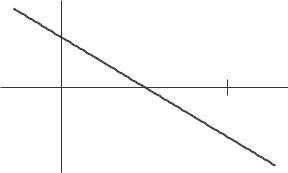
2 See Figure 2 44
33 See Figure 2 47
34 See Figure 2 48
35. See Figure 2 49
36. One possible graph is shown in Figure 2 50 Notice that as x gets large, the graph of f (x) gets more and more horizontal. Thus, as x gets large, f ′ (x) gets closer and closer to 0
37 See Figure 2 51
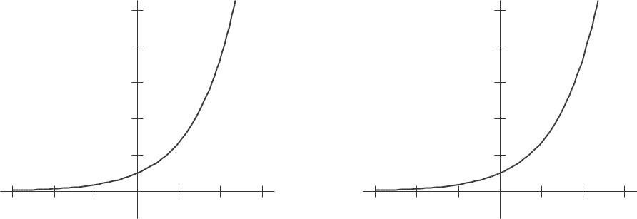
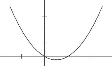
40. (a) Graph II (b) Graph I (c) Graph III
41.
42 The derivative is zero whenever the graph of the original function is horizontal Since the current is proportional to the derivative of the voltage, segments where the current is zero alternate with positive segments where the voltage is increasing and negative segments where the voltage is decreasing See Figure 2 54 Note that the derivative does not exist where the graph has a corner.