First course in statistics 11th edition mcclave solutions manual by carmen.hight310

Methods for Describing Sets of Data

2.2 In a bar graph, a bar or rectangle is drawn above each class of the qualitative variable corresponding to the class frequency or class relative frequency. In a pie chart, each slice of the pie corresponds to the relative frequency of a class of the qualitative variable.

2.4 First, we find the frequency of the grade A. The sum of the frequencies for all 5 grades must be 200. Therefore, subtract the sum of the frequencies of the other 4 grades from 200. The frequency for grade A is:

200 (36 + 90 + 30 + 28) = 200 184 = 16

To find the relative frequency for each grade, divide the frequency by the total sample size, 200. The relative frequency for the grade B is 36/200 = .18. The rest of the relative frequencies are found in a similar manner and appear in the table:

2.6

a. The graph shown is a pie chart.

b. The qualitative variable described in the graph is opinion on library importance.

c. The most common opinion is more important, with 46.0% of the responders indicating that they think libraries have become more important.

Methods for Describing Sets of Data 5

Grade on Statistics Exam Frequency Relative Frequency A: 90 100 16 .08 B: 80 89 36 .18 C: 65 79 90 .45 D: 50 64 30 .15 F: Below 50 28 .14 Total 200 1.00

Chapter 2 First Course in Statistics 11th Edition McClave Solutions Manual Visit TestBankDeal.com to get complete for all chapters

d. Using MINITAB, the Pareto diagram is:

Of those who responded to the question, almost half (46%) believe that libraries have become more important to their community. Only 18% believe that libraries have become less important.

2.8 a. Data were collected on 3 questions. For questions 1 and 2, the responses were either ‘yes’ or ‘no’. Since these are not numbers, the data are qualitative. For question 3, the responses include ‘character counts’, ‘roots of empathy’, ‘teacher designed’, other’, and ‘none’. Since these responses are not numbers, the data are qualitative.

b. Using MINITAB, bar charts for the 3 questions are:

Importance Percent Less Same More 50 40 30 20 10 0 Importance

Classroom Pets Count Yes No 60 50 40 30 20 10 0 Chart of Classroom Pets

c. Many different things can be written. Possible answers might be: Most of the classroom teachers surveyed (61/75 = .813) keep classroom pets. A little less than half of the surveyed classroom teachers (35/75 = .467) allow visits by pets.

2.10 a. A PIN pad is selected and the manufacturer is determined. Since manufacturer is not a number, the data collected are qualitative.

Methods for Describing Sets of Data 7

Pet Visits Count Yes No 40 30 20 10 0 Chart of Pet Visits Education Count None Other Teacher designed Roots of empathy Character counts 30 25 20 15 10 5 0 Chart of Education

b. Using MINITAB, the frequency bar chart is:

c. The Pareto chart for the data is:

Most of the PIN pads were shipped by Fujian Landi. They shipped almost twice as many PIN pads as the second highest manufacturer, which was SZZT Electronics. The three manufacturers with the smallest number of Pin pads shipped were Glintt, Intelligent, and Urmet.

2.12 a. The two qualitative variables graphed in the bar charts are the occupational titles of clan individuals in the continued line and the occupational titles of clan individuals in the dropout line.

8 Chapter 2 Copyright

Manufacturer Count Urmet Toshiba TEC SZZT Electronics ProvencoCadmus Pax Tech. Omron KwangWoo Intelligent Glintt Fujuan Landi CyberNet Bitel 120000 100000 80000 60000 40000 20000 0 Chart of Manufacturer

Manufacturer Count Urmet Intelligent Glintt Pax Tech. Toshiba TEC Bitel CyberNet ProvencoCadmus Omron KwangWoo SZZT Electronics Fujuan Landi 120000 100000 80000 60000 40000 20000 0 Chart of Manufacturer

b. In the Continued Line, about 63% were in either the high or the middle grade. Only about 20% were in the nonofficial category. In the Dropout Line, only about 22% were in either the high or middle grade while about 64% were in the nonofficial category. The percents in the low grade and provincial official categories were about the same for the two lines.

2.14 Suppose we construct a relative frequency bar chart for this data. This will allow the archaeologists to compare the different categories easier. First, we must compute the relative frequencies for the categories. These are found by dividing the frequencies in each category by the total 837. For the burnished category, the relative frequency is 133 / 837 = .159. The rest of the relative frequencies are found in a similar fashion and are listed in the table.

The most frequently found type of pot was the Monochrome. Of all the pots found, 55% were Monochrome. The next most frequently found type of pot was the Painted in Geometric Decoration. Of all the pots found, 19.7% were of this type. Very few pots of the types Painted in naturalistic decoration, Cycladic white clay, and Conical cup clay were found.

Methods for Describing Sets of Data 9

Pot Category Number Found Computation Relative Frequency Burnished 133 133 / 837 .159 Monochrome 460 460 / 837 .550 Slipped 55 55 / 837 .066 Curvilinear Decoration 14 14 / 837 .017 Geometric Decoration 165 165 / 837 .197 Naturalistic Decoration 4 4 / 837 .005 Cycladic White clay 4 4 / 837 .005 Cononical cup clay 2 2 / 837 .002 Total 837 1.001

relative

Pot Category Relative Frequency Conical Cycladic Naturalistic Geometric Curvilinear Slipped Monochrome Burnished .60 .48 .36 .24 .12 0

frequency bar chart is:

Chart of Pot Category

2.16 Using MINITAB, a bar graph is:

Most of the types of papers found were interviews. There were about twice as many interviews as all other types combined.

2.18 a. There were 1,470 responses that were missing. In addition, 14 responses were 8 = Don’t know and 7 responses were 9 = Missing. The missing values were not included, but those responding with an 8 were kept. Therefore, there were only 1333 useable responses. The frequency table is:

Fieldwork Count 4Grounded 3Observ 2Obs+Partic 1Interview 5000 4000 3000 2000 1000 0 Chart of Fieldwork

Response Frequency Relative Frequency 1 450 450/1333 = .338 2 627 627/1333 = .470 3 219 219/1333 = .164 4 23 23/1333 = .017 8 14 14/1333 = .011 Totals 1333 1.000

b. Using MINITAB, the pie chart for the data is:

c. The response with the highest frequency is 2, ‘the Bible is the inspired word of God but not everything is to be taken literally’. Almost 47% of the respondents selected this answer. About one-third of the respondents answered 1, ‘the Bible is the actual word of God and is to be taken literally’. Very few (1.7%) of the respondents chose response 4, ‘the Bible has some other origin’ and response 8 (1.1%), ‘Don’t know’.

2.20 Using MINITAB a bar chart for the Extinct status versus flight capability is:

It appears that extinct status is related to flight capability. For birds that do have flight capability, most of them are present. For those birds that do not have flight capability, most are extinct.

Methods for Describing Sets of Data 11

8 4 3 2 1 Category 8 1 2 3 4

Pie Chart of Bible Categories

Count Extinct Flight Extinct Present Absent Yes No Yes No Yes No 80 70 60 50 40 30 20 10 0 Chart of Extinct, Flight

The bar chart for Extinct status versus Nest Density is:

It appears that extinct status is not related to nest density. The proportion of birds present, absent, and extinct appears to be very similar for nest density high and nest density low.

The bar chart for Extinct status versus Habitat is:

It appears that the extinct status is related to habitat. For those in aerial terrestrial (TA), most species are present. For those in ground terrestrial (TG), most species are extinct. For those in aquatic, most species are present.

2.22 The difference between a bar chart and a histogram is that a bar chart is used for qualitative data and a histogram is used for quantitative data. For a bar chart, the categories of the qualitative variable usually appear on the horizontal axis. The frequency or relative frequency for each category usually appears on the vertical axis. For a histogram, values of the quantitative variable usually appear on the horizontal axis and either frequency or relative frequency usually appears on the vertical axis. The quantitative data are grouped into intervals which appear on the horizontal axis. The number of observations appearing in each interval is then graphed. Bar charts usually leave spaces between the bars while histograms do not.

Count Extinct Nest Density Extinct Present Absent L H L H L H 60 50 40 30 20 10 0 Chart of Extinct, Nest Density

Count Extinct Habitat Extinct Present Absent TG TA A TG TA A TG TA A 40 30 20 10 0 Chart of Extinct, Habitat

2.24 In a stem-and-leaf display, the stem is the left-most digits of a measurement, while the leaf is the right-most digit of a measurement.

2.26 As a general rule for data sets containing between 25 and 50 observations, we would use between 7 and 14 classes. Thus, for 50 observations, we would use around 14 classes.

2.28 Using MINITAB, the relative frequency histogram is:

2.30

a. This is a frequency histogram because the number of observations are displayed rather than the relative frequencies.

b. There are 14 class intervals used in this histogram.

c. The total number of measurements in the data set is 49.

2.32 a. Using MINITAB, the dot plot of the honey dosage data is:

Dotplot of Honey Dosage Group

b. Both 10 and 12 occurred 6 times in the honey dosage group.

Methods for Describing Sets of Data 13

Class Interval Relative frequency 16.5 14.5 12.5 10.5 8.5 6.5 4.5 2.5 0.5 .25 .20 .15 .10 .05 0

ImproveScore 16 14 12 10 8 6 4

c. From the graph in part c, 8 of the top 11 scores (72.7%) are from the honey dosage group. Of the top 30 scores, 18 (60%) are from the honey dosage group. This supports the conclusions of the researchers that honey may be a preferable treatment for the cough and sleep difficulty associated with childhood upper respiratory tract infection.

2.34 Using MINITAB, the stem-and-leaf display is:

Stem-and-Leaf Display: Depth

Stem-and-leaf of Depth N = 18

Leaf Unit = 0.10

2 13 29

4 14 00

8 15 7789

(3) 16 125

7 17 08

5 18 11

3 19 347

The data in the stem-and-leaf display are displayed to 1 decimal place while the actual data is displayed to 2 decimal places. To 1 decimal place, there are 3 numbers that appear twice –14.0, 15.7, and 18.1. However, to 2 decimal places, none of these numbers are the same. Thus, no molar depth occurs more frequently in the data.

2.36 a. Using MINITAB, the dot plot for the 9 measurements is:

b. Using MINITAB, the stem-and-leaf display is:

Character Stem-and-Leaf Display

Stem-and-leaf of Cesium N = 9

Leaf Unit = 0.10 1

14 Chapter 2

Cesium -4.2 -4.5 -4.8 -5.1 -5.4 -5.7 -6.0 Dotplot of Cesium

-6 0

-5 5

-5

-4

00 (3) -4 865 2

2.38

c. Using MINITAB, the histogram is:

d. The stem-and-leaf display appears to be more informative than the other graphs. Since there are only 9 observations, the histogram and dot plot have very few observations per category.

e. There are 4 observations with radioactivity level of -5.00 or lower. The proportion of measurements with a radioactivity level of -5.0 or lower is 4 / 9 = .444.

a. Using MINITAB, the stem-and-leaf display is:

Stem-and-Leaf Display: Spider

Stem-and-leaf of Spider N = 10 Leaf Unit = 10

b. The spiders with a contrast value of 70 or higher are in bold type in the stem-and-leaf display in part a. There are 3 spiders in this group.

c. The sample proportion of spiders that a bird could detect is 3 / 10 = .3. Thus, we could infer that a bird could detect a crab-spider sitting on the yellow central part of a daisy about 30% of the time.

Methods for Describing Sets of Data 15

Cesium Frequency -4.0 -4.5 -5.0 -5.5 -6.0 2.0 1.5 1.0 0.5 0.0 Histogram of Cesium

1 0 0 3 0 33 (3) 0 455 4 0 67 2 0 9 1 1 1

2.40 a. A stem-and-leaf display of the data using MINITAB is: Stem-and-leaf of FNE N = 25

= 1.0

b. The numbers in bold in the stem-and-leaf display represent the bulimic students. Those numbers tend to be the larger numbers. The larger numbers indicate a greater fear of negative evaluation. Thus, the bulimic students tend to have a greater fear of negative evaluation.

c. A measure of reliability indicates how certain one is that the conclusion drawn is correct. Without a measure of reliability, anyone could just guess at a conclusion.

2.42 a. Using MINITAB, histograms of the two sets of SAT scores are:

It appears that the distributions of both sets of scores are somewhat skewed to the right. However, there appears to be more lower SAT scores for 2009 and more higher SAT scores for 2009 than 2005.

16 Chapter 2

Leaf Unit

2 0 67 3 0 8 6 1 001 10 1 3333 12 1 45 (2) 1 66 11 1 8999 7 2 0011 3 2 3 2 2 45

Frequency 1200 1120 1040 960 18 16 14 12 10 8 6 4 2 0 1200 1120 1040 960 SAT2005 SAT2009 Histogram of SAT2005, SAT2009

b. Using MINITAB, a histogram of the differences of the 2009 and 2005 SAT scores is:

c. It appears that there are more differences less than 0 than above 0. Thus, it appears that in general, the 2009 SAT scores are lower than the 2005 SAT scores.

d. Wyoming had the largest improvement in SAT scores from 2005 to 2009, with an increase of 48 points. 2.44 a. 5132112 x =++++=

b. 2222225132140 x =++++=

c. (1)(51)(11)(31)(21)(11)7 x −=−+−+−+−+−=

d. 222222 (1)(51)(11)(31)(21)(11)21 x

2.46 Using the results from Exercise 2.44,

b. 222222 (2)(52)(12)(32)(22)(12)12 x −=−+−+−+−+−=

c. 2 10401030 x −=−=

Methods for Describing Sets of Data 17

Diff Frequency 40 20 0 -20 -40 -60 -80 20 15 10 5 0 Histogram of Diff

∑

=++++== ∑ = (5 + 1 + 3 + 2 + 1)2 = 122 = 144

−=−+−+−+−+−=

e. ()

22 (51321)12144 x

−=−=−= ∑ ∑

a. () 2 2 144 404028.811.2 55 x x

∑

2.48 A measure of central tendency measures the “center” of the distribution while measures of variability measure how spread out the data are.

2.50 The sample mean is represented by x . The population mean is represented by µ

2.52 A skewed distribution is a distribution that is not symmetric and not centered around the mean. One tail of the distribution is longer than the other. If the mean is greater than the median, then the distribution is skewed to the right. If the mean is less than the median, the distribution is skewed to the left.

2.54 Assume the data are a sample. The sample mean is:

3.22.52.13.72.82.016.3 2.717 66 x x n +++++

The median is the average of the middle two numbers when the data are arranged in order (since n = 6 is even). The data arranged in order are: 2.0, 2.1, 2.5, 2.8, 3.2, 3.7. The middle two numbers are 2.5 and 2.8. The median is:

2.52.85.3 2.65 22 + ==

2.56 The median is the middle number once the data have been arranged in order. If n is even, there is not a single middle number. Thus, to compute the median, we take the average of the middle two numbers. If n is odd, there is a single middle number. The median is this middle number.

A data set with 5 measurements arranged in order is 1, 3, 5, 6, 8. The median is the middle number, which is 5.

A data set with 6 measurements arranged in order is 1, 3, 5, 5, 6, 8. The median is the average of the middle two numbers which is 5 2 10

Median = 33 3 2 + = (mean of 3rd and 4th numbers, after ordering)

Median = 3 (7th number, after ordering)

Median = 4850 49 2 + = (mean of 5th and 6th numbers, after ordering)

18 Chapter 2

∑

====

2.58 a. 7415 2.5 66 x x n ++ ==== ∑

2 5 5 = = + .

2440

1313 x x n

==== ∑

= 3

5137496

1010 x x n

==== ∑

Mode = 3 b.

3.08

Mode

49.6

Mode = 50

2.60 a. From the printout, the sample mean is 50.02, the sample median is 51, and the sample mode is 54. The average age of the 50 most powerful women in business in the U.S. is 50.02 years. The median age is 51. Half of the 50 most powerful women in business in the U.S. are younger than 51 and half are older. The most common age is 54.

b. Since the mean is slightly smaller than the median, the data are skewed slightly to the left.

c. The modal class is the interval with the largest frequency. From the histogram the modal class is 50 to 54.

2.62 a. There are 35 observations in the honey dosage group. Thus, the median is the middle number, once the data have been arranged in order from the smallest to the largest. The middle number is the 18th observation which is 11.

b. There are 33 observations in the DM dosage group. Thus, the median is the middle number, once the data have been arranged in order from the smallest to the largest. The middle number is the 17th observation which is 9.

c. There are 37 observations in the control group. Thus, the median is the middle number, once the data have been arranged in order from the smallest to the largest. The middle number is the 19th observation which is 7.

d. Since the median of the honey dosage group is the highest, the median of the DM groups is the next highest, and the median of the control group is the smallest, we can conclude that the honey dosage is the most effective, the DM dosage is the next most effective, and nothing (control) is the least effective.

2.64

a. The mean of the driving performance index values is:

The median is the average of the middle two numbers once the data have been arranged in order. After arranging the numbers in order, the 20th and 21st numbers are 1.75 and 1.76. The median is: 755 1 2 76 1 75 1 = +

The mode is the number that occurs the most frequently and is 1.4.

b. The average driving performance index is 1.927. The median is 1.755. Half of the players have driving performance index values less than 1.755 and half have values greater than 1.755. Three of the players have the same index value of 1.4.

Methods for Describing Sets of Data 19

927 1 40 77.07 = = = ∑ n x x

c. Since the mean is greater than the median, the data are skewed to the right. Using MINITAB, a histogram of the data is:

2.66 a. The salaries of all persons employed by a large university are probably skewed to the right. There will be a few individuals with very large salaries (i.e. president, football coach, Dean of the Medical school). However, the majority of the employees will have salaries in a rather small range.

b. The grades on an easy test will probably be skewed to the left. Most students will get very high grades on the test. Since there is an upper limit to the grades (i.e. 100%), there will likely be many grades in this upper range. However, even on an easy test, a few individuals will still not do well.

c. The grades on a difficult test will probably be skewed to the right. Most students will get fairly low grades on the test. However, even on a difficult test, a few individuals will still do quite well.

d. The amounts of time students in your class studied last week will probably be close to symmetric. Some individuals will not study very much, while others will study quite a bit. However, most students will study an average amount of time.

e. The ages of cars on a used car lot will probably be skewed to the left. Most of the cars will be fairly new. However, there will probably be a few fairly old cars.

f. The amounts of time spent by students on a difficult examination will probably be skewed to the left. If there is a maximum time limit, then most students will take that amount of time or close to it. There will probably be a few students who take less time than the maximum allowed.

Education, Inc.

2013 Pearson

Performance Frequency 3.5 3.0 2.5 2.0 1.5 10 8 6 4 2 0 Histogram of Performance

2.68 a. The mean number of ant species discovered is:

33...4141 12.82 1111 x

The median is the middle number once the data have been arranged in order: 3, 3, 4, 4, 4, 5, 5, 5, 7, 49, 52.

The median is 5.

The mode is the value with the highest frequency. Since both 4 and 5 occur 3 times, both 4 and 5 are modes.

b. For this case, we would recommend that the median is a better measure of central tendency than the mean. There are 2 very large numbers compared to the rest. The mean is greatly affected by these 2 numbers, while the median is not.

c. The mean total plant cover percentage for the Dry Steppe region is:

4052...27202 40.4

The median is the middle number once the data have been arranged in order: 27, 40, 40, 43, 52.

The median is 40.

The mode is the value with the highest frequency. Since 40 occurs 2 times, 40 is the mode.

d. The mean total plant cover percentage for the Gobi Desert region is:

3016...14168 28 66 x x n +++ ====

The median is the mean of the middle 2 numbers once the data have been arranged in order: 14, 16, 22, 30, 30, 56.

The median is 223052 26 22 + ==

The mode is the value with the highest frequency. Since 30 occurs 2 times, 30 is the mode.

e. Yes, the total plant cover percentage distributions appear to be different for the 2 regions. The percentage of plant coverage in the Dry Steppe region is much greater than that in the Gobi Desert region.

Methods for Describing Sets of Data 21

∑

x n +++ ====

∑

55 x x n +++ ====

∑

2.70 a. The mean number of power plants is:

The median is the mean of the middle 2 numbers once the data have been arranged in order:

The median is 347 3.5 22 + == .

The number 1 occurs 5 times. The mode is 1.

b. Deleting the largest number, 11, the new mean is:

The median is the middle number once the data have been arranged in order:

The median is 3.

The number 1 occurs 5 times. The mode is 1.

By dropping the largest measurement from the data set, the mean drops from 3.9 to 3.526. The median drops from 3.5 to 3 and the mode stays the same.

c. Deleting the lowest 2 and highest 2 measurements leaves the following:

The new mean is:

111...756 3.5 1616

The trimmed mean has the advantage that some possible outliers have been eliminated.

2.72 The primary disadvantage of using the range to compare variability of data sets is that the two data sets can have the same range and be vastly different with respect to data variation. Also, the range is greatly affected by extreme measures.

2.74 The variance of a data set can never be negative. The variance of a sample is the sum of the squared deviations from the mean divided by n 1. The square of any number, positive or negative, is always positive. Thus, the variance will be positive.

Pearson Education, Inc.

2013

2020 n i i x x n =

==== ∑

524...378 3.9

++++

1, 1, 1, 1, 2, 2, 3, 3, 3, 4, 4, 4, 5, 5, 5, 6, 7, 9,

n i i x x n =

==== ∑

524...367 3.526 1919

++++

1, 1, 1, 1, 1, 2, 2, 3, 3, 3, 4, 4, 4, 5, 5, 5, 6, 7, 9

1, 1, 1, 2, 2, 3, 3, 3, 4, 4, 4, 5, 5, 5, 6, 7

n i i x x n =

==== ∑

++++

The variance is usually greater than the standard deviation. However, it is possible for the variance to be smaller than the standard deviation. If the data are between 0 and 1, the variance will be smaller than the standard deviation. For example, suppose the data set is .8, .7, .9, .5, and .3. The sample mean is:

Methods for Describing Sets of Data 23

.8.7.9.5.33.2 .64 .55 x x n ++++ ==== ∑ The sample variance is: () 2 2 2 2 3.2 2.28 2.282.048 5 .058 1514 x x n s n ==== ∑ ∑ The standard deviation is .058.241 s == 2.76 a. () 2 2 2 2 20 84 10 4.8889 1101 x x n s n === ∑ ∑ 4.88892.211 s == b. () 2 2 2 2 100 380 40 3.3333 1401 x x n s n === ∑ ∑ 3.33331.826 s == c. () 2 2 2 2 17 18 20 .1868 1201 x x n s n === ∑ ∑ .1868.432 s == 2.78 a. Range = 4 0 = 4 () 2 2 2 2 8 22 5 2.3 141 x x n s n === ∑ ∑ 2.31.52 s == b. Range = 6 0 = 6 () 2 2 2 2 17 63 7 3.619 171 x x n s n === ∑ ∑ 3.6191.90 s ==

2.80 This is one possibility for the two data sets.

The two sets of data above have the same range = largest measurement smallest measurement = 9 0 = 9.

The means for the two data sets are:

The dot diagrams for the two data sets are shown below.

= 8 ( 2) = 10 () 2 2 2 2 27 145 9 8 191 x x n s n === ∑ ∑ 82.828 s ==

( 3) = 5 () 2 2 2 2 (5) 29 18 1.624 1181 x x n s n === ∑ ∑ 1.6241.274 s ==

c. Range

d. Range = 2

Data Set 1: 0, 1, 2, 3, 4, 5, 6, 7, 8, 9 Data Set 2: 0, 0, 1, 1, 2, 2, 3, 3, 9, 9

1 012345678945 4.5 1010 x x n = +++++++++ === ∑ 2 001122339930 3 1010 x x n +++++++++ ==== ∑

Data Group 8 6 4 2 0 1 2 x-bar x-bar Dotplot of Data vs Group 2.82 a. () 2 2 2 2 28 226 69.2 5 17.3 1514 x x n s n ==== ∑ ∑ 17.34.1593 s ==

2.84

a. For those students who earned A, the range is 53 – 24 = 29.

2.86

b. For those students who earned a B or C, the range is 40 – 16 = 24.

c. The students who received A’s have a more variable distribution of the number of books read. The range, variance, and standard deviation for this group are greater than the corresponding values for the B-C group

a. The range is the difference between the largest and smallest observations and is 17.83 –4.90 = 12.93 meters.

b. The variance is:

c. The standard deviation is 16.7674.095 s == meters.

Education,

b. () 2 2 2 2 55 1213 456.75 4 152.25 1413 x x n s n ==== ∑ ∑ square feet 152.2512.339 s == feet c. () 2 2 2 2 (15) 59 21.5 6 4.3 1615 x x n s n ==== ∑ ∑ 4.32.0736 s == d. () 2 2 2 2 242 .2933 256 .0587 1615 x x n s n ==== ∑ ∑ square ounces .0587.2422 s == ounce

Pearson

Inc.

The variance is () 2 2 2 2 296 11,482 530 8 75.7143 177 x x n s n ==== ∑ ∑ The standard deviation

2 75.71438.701 ss=== .

The variance is () 2 2 2 2 147 3,965 363.5 6 72.7 155 x x n s n ==== ∑ ∑ The standard deviation is 2 72.78.526 ss=== .

() 2 2 2 2 126.32 1428.64 13 16.767 square meters 1131 x x n s n === ∑ ∑

2.88 a. The maximum age is 64. The minimum age is 28. The range is 64 – 28 = 36.

b. The variance is:

c. The standard deviation is:

d. Since the standard deviation of the ages of the 50 most powerful women in Europe is 10 years and is greater than that in the U.S. (6.444 years), the age data for Europe is more variable.

e. If the largest age (64) is omitted, then the standard deviation would decrease. The new variance is:

The new standard deviation is 2 38.2416.184 ss=== . This is less than the standard deviation with all the observations (s = 6.444).

2.90 Chebyshev's rule can be applied to any data set. The Empirical Rule applies only to data sets that are mound-shaped—that are approximately symmetric, with a clustering of measurements about the midpoint of the distribution and that tail off as one moves away from the center of the distribution.

2.92 Since no information is given about the data set, we can only use Chebyshev's rule.

a. Nothing can be said about the percentage of measurements which will fall between xs and xs + .

b. At least 3/4 or 75% of the measurements will fall between 2 xs and 2 xs + .

c. At least 8/9 or 89% of the measurements will fall between 3 xs and 3 xs +

() 2 2 2 2 2501 127135 50 41.530 1501 x x n s n === ∑ ∑

41.536.444 ss===

() 2 2 2 2 2437 123039 49 38.241 1491 x x n s n === ∑ ∑

2.94 a. 206 8.24 25 x x n === ∑ () 2 2 2 2 206 1778 25 3.357 1251 x x n s n === ∑ ∑ 2 1.83 ss==

c. The percentages in part b are in agreement with Chebyshev's rule and agree fairly well with the percentages given by the Empirical Rule.

d. Range = 12 5 = 7

s ≈ range/4 = 7/4 = 1.75

The range approximation provides a satisfactory estimate of s

2.96 From Exercise 2.60, the sample mean is 50.02 x = . From Exercise 2.88, the sample standard deviation is s = 6.444. From Chebyshev’s Rule, at least 75% of the ages will fall within 2 standard deviations of the mean. This interval will be:

2.98 a. If the data are symmetric and mound shaped, then the Empirical Rule will describe the data. About 95% of the observations will fall within 2 standard deviation of the mean. The interval two standard deviations below and above the mean is 2392(6)3912(27,51)

xs ± ⇒ ± ⇒ ± ⇒ . This range would be 27 to 51.

b. To find the number of standard deviations above the mean a score of 51 would be, we subtract the mean from 51 and divide by the standard deviation. Thus, a score of 51 is 5139 2 6 = standard deviations above the mean. From the Empirical Rule, about .025 of the drug dealers will have WR scores above 51.

c. By the Empirical Rule, about 99.7% of the observations will fall within 3 standard deviations of the mean. Thus, nearly all the scores will fall within 3 standard deviations of the mean. The interval three standard deviations below and above the mean is 3393(6)3918(21,57)

xs ± ⇒ ± ⇒ ± ⇒ . This range would be 21 to 57.

2.100 a. 213.22(19.5)13.239(25.8,52.2)xs ± ⇒ ± ⇒ ± ⇒ . Since time cannot be negative, the interval will be (0,52.2) .

b. The number of minutes a student uses a laptop for taking notes each day must be a positive number. The standard deviation is larger than the mean. Thus, even one standard deviation below the mean is a negative number. This implies that the distribution cannot be symmetric.

Methods for Describing Sets of Data 27

Interval Number of Measurements in Interval Percentage xs ± , or (6.41, 10.07) 18 18/25 = .72 or 72% 2 xs ± , or (4.58, 11.90) 24 24/25 = .96 or 96% 3 xs ± , or (2.75, 13.73) 25 25/25 = 1 or 100%

250.022(6.444)50.0212.888(37.132,62.908)xs ± ⇒ ± ⇒ ± ⇒

c. Since we know the distribution of usage times cannot be symmetric, we can use Chebyshev’s Rule. We know that at least ¾ or 75% of the observations will be within 2 standard deviations of the mean. Thus, we know that at least 75% of the students have laptop usages between -25.8 and 52.2 minutes per day. Since we know we cannot have negative usages, the interval will be from 0 to 52.2 minutes.

2.102 a. There are 2 observations with missing values for egg length, so there are only 130 useable observations.

b. The data are not symmetrical or mound-shaped. Thus, we will use Chebyshev’s Rule. We know that there are at least 8/9 or 88.9% of the observations within 3 standard deviations of the mean. Thus, at least 88.9% of the observations will fall in the interval:

360.653(43.99)60.65131.97(71.32, 192.69)

Since it is impossible to have negative egg lengths, at least 88.9% of the egg lengths will be between 0 and 192.69.

2.104 If we assume that the distributions are symmetric and mound-shaped, then the Empirical Rule will describe the data. We will compute the mean plus or minus one, two and three standard deviations for both data sets:

28 Chapter 2

7,885 60.65 130 x x n ∑ === () 2 2 2 2 (7,885) 727,842 249,586.4231 130 1,934.7785 11301129 x x n s n ==== ∑ ∑ 2 1,934.778543.99 ss===

xs ± ⇒ ± ⇒ ± ⇒

Low income: 7.628.91(1.29,16.53) xs ± ⇒ ± ⇒ 27.622(8.91)7.6217.82(10.20,25.44)xs ± ⇒ ± ⇒ ± ⇒ 37.623(8.91)7.6226.73(19.11,34.35)xs ± ⇒ ± ⇒ ± ⇒ Middle Income: 15.5512.24(3.31,27.79) xs ± ⇒ ± ⇒ 215.552(12.24)15.5524.48(8.93,40.03)xs ± ⇒ ± ⇒ ± ⇒ 315.553(12.24)15.5536.72(21.17,52.27)xs ± ⇒ ± ⇒ ± ⇒

The histogram for the middle income group is as follows: .35 .30 .25 .20 .15 .10 .05

The histogram for the low income group is as follows: Relatie frequency 52.27 40.03 27.79 15.55 3.31 -8.93 -21.17

The spread of the data for the middle income group is much larger than that of the low income group. The middle of the distribution for the middle income group is 15.55, while the middle of the distribution for the low income group is 7.62. Thus, the middle of the distribution for the middle income group is shifted to the right of that for the low income group.

We might be able to compare the means for the two groups. From the data provided, it looks like the mean score for the middle income group is greater than the mean score for the lower income group.

Methods for Describing Sets of Data 29

Complexity Relatie frequency 34.35 25.44 16.53 7.62 -1.29 -10.00 -19.11 .35 .30 .25 .20 .15 .10 .05

(Note: From looking at the data, it is rather evident that the distributions are not moundshaped and symmetric. For the low income group, the standard deviation is larger than the mean. Since the smallest measurement allowed is 0, this indicates that the data set is not symmetric but skewed to the right. A similar argument could be used to indicate that the data set of middle income scores is also skewed to the right.)

2.106 To decide which group the patient is most likely to come from, we will compute the z-score for each group.

The patient is most likely to have come from Group T. The z-score for Group T is z = 1.58. This would not be an unusual z-score if the patient was in Group T. The z-scores for the other 2 groups are both greater than 2. We know that z-scores greater than 2 are rather unusual.

2.108 a. The 50th percentile is also called the median.

b. The QL is the lower quartile. This is also the 25th percentile or the score which has 25% of the observations less than it.

c. The QU is the upper quartile. This is also the 75th percentile or the score which has 75% of the observations less than it.

2.110 For mound-shaped distributions, we can use the Empirical Rule. About 95% of the observations will fall within 2 standard deviations of the mean. Thus, about 95% of the measurements will have z-scores between -2 and 2.

2.112 We first compute z-scores for each x value.

The above z-scores indicate that the x value in part a lies the greatest distance above the mean and the x value of part b lies the greatest distance below the mean.

Group T: 58 1 6 7 10.5 22.5 = = = σ µ x z Group V: 48 2 5 7 9 3 5 22 = = = σ µ x z Group C: 81 2 5 7 4 1 5 22 = = = σ µ x z

a. 10050 2 25 x z µ σ === b. 14 3 1 x z µ σ ===− c. 0200 2 100 x z µ σ ===− d. 105 1.67 3 x z µ σ ===

2.114 The mean score is 283. This is the arithmetic average score of U.S. eighth graders on the mathematics assessment test. The 25th percentile score is 259. This indicates that 25% of the U.S. eighth graders scored 259 or lower on the assessment test. The 75th percentile score is 308. This indicates that 75% of the U.S. eighth graders scored 308 or lower on the assessment test. The 90th percentile score is 329. This indicates that 90% of the U.S. eighth graders scored 329 or lower on the assessment test.

2.116 From Exercise 2.35, 95.699 x = and s = 4.963.

a. The z-score for the Nautilus Explorer is:

The score for the Nautilus Explorer is 4.37 standard deviations below the mean for all the cruise ships.

b. The z-score for the Rotterdam is:

The score for the Rotterdam is 0.75 standard deviations below the mean for all the cruise ships.

2.118 a. The mean number of books read by students who earned an A grade is:

From Exercise 2.84, s = 8.701.

8.701 xx z s === . Thus, someone who read 40 books read more than the average number of books, but that number is not very unusual.

The z-score for a score of 40 books is

b. The mean number of books read by students who earned a B or C grade is:

147 24.5 6 x x n ===

From Exercise 2.84, s = 8.526.

The z-score for a score of 40 books is 4024.5 1.82 8.526 xx z s === . Thus, someone who read 40 books read many more than the average number of books. Very few students who received a B or a C read more than 40 books.

c. The group of students who earned A’s is more likely to have read 40 books. For this group, the z-score corresponding to 40 books is .34. This is not unusual. For the B-C group, the z-score corresponding to 40 books is 1.82. This is close to 2 standard deviations from the mean. This would be fairly unusual.

Methods for Describing Sets of Data 31

7495.699

4.963 xx z s

4.37

===−

9295.699 0.75 4.963 xx z s ===−

296 37

∑

8 x x n ===

4037

0.34

∑

2.120 Since the 90th percentile of the s less than the USEPA level of .01 of drinking water with unhealthy

study sample in the subdivision was .00372 mg/L, whi 15 mg/L, the water customers in the subdivision are no y lead levels.

2.122 a. If the distribution is mound

Approximately 68% of the between 53% ± 15% or bet fall within 2 standard devia and 83%. Approximately a mean or between 53% ± 3(

d-shaped and symmetric, then the Empirical Rule can e scores will fall within 1 standard deviation of the mea tween 38% and 68%. Approximately 95% of the scor ations of the mean or between 53% ± 2(15%) or betwe all of the scores will fall within 3 standard deviations o (15%) or between 8% and 98%.

b. If the distribution is mound

Approximately 68% of the between 39% ± 12% or bet fall within 2 standard devia and 63%. Approximately a mean or between 39% ± 3(

d-shaped and symmetric, then the Empirical Rule can e scores will fall within 1 standard deviation of the mea tween 27% and 51%. Approximately 95% of the scor ations of the mean or between 39% ± 2(12%) or betwe all of the scores will fall within 3 standard deviations o (12%) or between 3% and 75%.

c. Since the scores on the red score of 20% is more likely

d exam are shifted to the left of those on the blue exam y to occur on the red exam than on the blue exam.

2.124 Yes. From the graph in Exercise scores greater than 3. There is th different from the rest of the dat know that by ranking the data, w loose valuable information.

e 2.121 c, we can see that there are 4 observations wit hen a gap down to 2.18. Those 4 observations are qui ta. After those 4 observations, the data are fairly simil we can reduce the influence of outliers. But, by doing t

2.126 The interquartile range is the dis

stance between the upper and lower quartiles.

2.128 For a mound-shaped distribution observations will fall within 3 st observations will have z-scores b

n, the Empirical Rule can be used. Almost all of the tandard deviations of the mean. Thus, almost all of the between -3 and 3.

2.130 The interquartile range is IQR =

QU QL = 85 60 = 25.

The lower inner fence = QL 1.5

The upper inner fence = QU + 1.

The lower outer fence = QL 3(

5(IQR) = 60 1.5(25) = 22.5.

5(IQR) = 85 + 1.5(25) = 122.5.

(IQR) = 60 3(25) = 15.

The upper outer fence = QU + 3(

(IQR) = 85 + 3(25) = 160.

With only this information, the b

box plot would look something like the following:

ch is t at risk be used. n or es will en 23% f the be used. n or es will en 15% f the , a h zte ar. We his, we

32 Chapter 2 Copyright

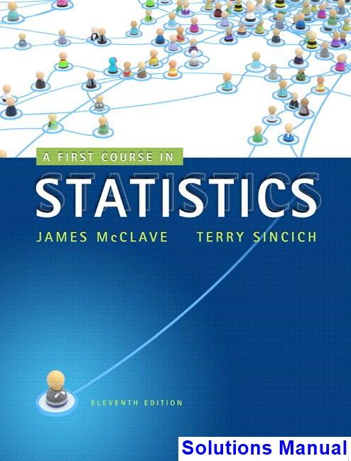
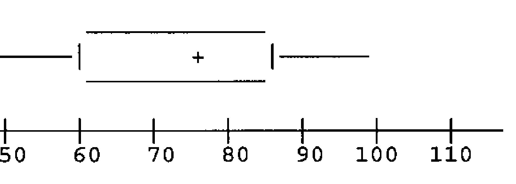
The whiskers extend to the inner fences unless no data points are that small or that large. The upper inner fence is 122.5. However, the largest data point is 100, so the whisker stops at 100. The lower inner fence is 22.5. The smallest data point is 18, so the whisker extends to 22.5. Since 18 is between the inner and outer fences, it is designated with a *. We do not know if there is any more than one data point below 22.5, so we cannot be sure that the box plot is entirely correct.

2.132 a. Using Minitab, the box plot for sample A is given below.

Using Minitab, the box plot for sample B is given below.

b. In sample A, the measurements 84 and 100 are outliers. These measurements fall outside the outer fences.

Lower outer fence = Lower hinge 3(IQR)

≈ 158 3(172 158) = 158 3(14) = 116

In addition, 122 and 196 may be outliers. They lie outside the inner fences. In sample B, 140.4 and 206.4 may be outliers. They lie outside the inner fences.

Methods for Describing Sets of Data 33

Sample A 200 175 150 125 100 Boxplot of Sample A

Sample B 210 200 190 180 170 160 150 140 Boxplot of Sample B

b. Yes, we would consider this measurement an outlier. Any observation with a z-score that has an absolute value greater than 3 is considered a highly suspect outlier.

b. Yes, I would consider the z-score associated with the largest ratio to be unusually large. We know if the data are approximately mound-shaped that approximately 95% of the observations will be within 2 standard deviations of the mean. A z -score of 2.45 would indicate that less than 2.5% of all the measurements will be larger than this value.

c. Using MINITAB, the box plot is:

From this box plot, there are no observations marked as outliers.

2.136 a. The z-score associated with the largest ratio is 45 2 63439 5069 3 06 5 = = = s x x z The z-score associated with the smallest ratio is 98 1 63439 5069 3 25 2 = = = s x x z The z-score associated with the mean ratio is 0 63439 5069 3 5069 3 = = = s x x z

Tillratio 5.0 4.5 4.0 3.5 3.0 2.5 2.0 Boxplot of Tillratio

2.138 Using MINITAB, a boxplot of the data is:

From the boxplot, there is no indication that there are any outliers. We will now use the z-score criterion for determining outliers. From Exercises 2.59 and 2.86,

= and s = 4.095. The z-score associated with the minimum value is

===− and the z-score associated with the maximum value is

. Neither of these indicates there are any outliers.

2.140 a. Using MINITAB, the boxplots of the three groups are:

of Honey, DM, Control

b. The median improvement score for the honey dosage group is larger than the median improvement scores for the other two groups. The median improvement score for the DM dosage group is higher than the median improvement score for the control group.

Methods for Describing Sets of Data 35

Rockfall 17.5 15.0 12.5 10.0 7.5 5.0 Boxplot of

Rockfall

4.99.72 1.18 4.095

z s

17.839.72 1.98 4.095 xx z s ===

9.72 x

16 12 8 4 0 16 12 8 4 0 Honey DM Control Boxplot

c. Because the interquartile range for the DM dosage group is larger than the interquartile ranges of the other 2 groups, the variability of the DM group is largest. The variability of the honey dosage group and the control group appear to be about the same.

d. There appears to be one outlier in the honey dosage group and one outlier in the control group.

b. The z-score is low enough to suspect that the librarian's claim is incorrect. Even without any knowledge of the shape of the distribution, Chebyshev's rule states that at least 8/9 of the measurements will fall within 3 standard deviations of the mean (and, consequently, at most 1/9 will be above z = 3 or below z = 3).

c. The Empirical Rule states that almost none of the measurements should be above z = 3 or below z = 3. Hence, the librarian's claim is even more unlikely.

This is not an unlikely occurrence, whether or not the data are mound-shaped. Hence, we would not have reason to doubt the librarian's claim.

2.144 Scatterplots are useful with quantitative variables.

2.146 Using MINITAB, the scatterplot is as follows:

It appears that as variable 1 increases, variable 2 also increases.

36 Chapter 2

a. 47 3 1 x z µ σ ===−

2.142

When 2 σ = , 47 1.5 2 x z µ σ ===−

Variable 1 Variable 2 5 4 3 2 1 0 18 16 14 12 10 8 6 4 2 0 Scatterplot of Variable 2 vs Variable 1

2.148 Using MINITAB, a scatter plot of the data is:

2.150

If one uses the one obvious outlier (Denver), then there does appear to be a trend in the data. As the elevation increases, the slugging percentage tends to increase. However, if the outlier is removed, then it does not look like there is a trend to the data.

b. There appears to be a trend. As the age increases, the number of strikes tends to decrease.

Methods for Describing Sets of Data 37

ELEVATION SLUGPCT 6000 5000 4000 3000 2000 1000 0 0.625 0.600 0.575 0.550 0.525 0.500 0.475 0.450 Scatterplot of

SLUGPCT vs

ELEVATION

Age Strikes 190 180 170 160 150 140 130 120 90 80 70 60 50 40 30 20 10 Scatterplot of Strikes vs Age

a. A scattergram of the data is:

2.152 Using MINITAB, a scatterplot of the data is:

There is an increasing trend and there is very little variation in the plot. This supports the researcher’s theory.

2.154 a. Using MINITAB, the scatterplot of JIF and cost is:

There does not appear to be much of a trend between these two variables.

Resonance Freq 25 20 15 10 5 0 7000 6000 5000 4000 3000 2000 1000 Scatterplot of Freq vs Resonance

Cost JIF 1800 1600 1400 1200 1000 800 600 400 200 0 3.5 3.0 2.5 2.0 1.5 1.0 0.5 0.0 Scatterplot of JIF vs Cost

b. Using MINITAB, the scatterplot of cites and cost is:

There appears to be a positive linear trend between cites and cost.

c. Using MINITAB, the scatterplot of RPI and cost is:

There appears to be a positive linear trend between RPI and cost.

Methods for Describing Sets of Data 39

Cost Cites 1800 1600 1400 1200 1000 800 600 400 200 0 800 700 600 500 400 300 200 100 0 Scatterplot of Cites vs Cost

Cost RPI 1800 1600 1400 1200 1000 800 600 400 200 0 4 3 2 1 0 Scatterplot of RPI vs Cost

2.156 a. Using MINITAB, a graph of the Anthropogenic Index against the Natural Origin Index is:

This graph does not support the theory that there is a straight-line relationship between the Anthropogenic Index against the Natural Origin Index. There are several points that do not lie on a straight line.

b. After deleting the three forests with the largest anthropogenic indices, the graph of the data is:

After deleting the 3 data points, the relationship between the Anthropogenic Index against the Natural Origin Index is much closer to a straight line.

F-Natural F-Anthro 40 35 30 25 20 15 10 5 90 80 70 60 50 40 30 20 10 0 Scatterplot of F-Anthro vs F-Natural

F-Natural F-Anthro 40 35 30 25 20 15 10 5 60 50 40 30 20 10 0 Scatterplot of F-Anthro vs F-Natural

2.158 Using MINITAB, a scattergram of the data is:

Yes, there appears to be a negative trend in this data. As time increases, the mass tends to decrease. There appears to be a curvilinear relationship. As time increases, mass decreases at a decreasing rate.

2.160 The range can be greatly affected by extreme measures, while the standard deviation is not as affected.

2.162 The z-score approach for detecting outliers is based on the distribution being fairly moundshaped. If the data are not mound-shaped, then the box plot would be preferred over the zscore method for detecting outliers.

2.164 The relative frequency histogram is:

Methods for Describing Sets of Data 41

Time Mass 60 50 40 30 20 10 0 7 6 5 4 3 2 1 0 Scatterplot of Mass vs Time

Class Interval Percent 9.00 8.25 7.50 6.75 6.00 5.25 4.50 3.75 3.00 2.25 1.50 0.75 0.00 20 15 10 5 0 Histogram of Class Interval

2.166 From part a of Exercise 2.165, the 3 z-scores are 1, 1 and 2. Since none of these z-scores are greater than 2 in absolute value, none of them are outliers.

From part b of Exercise 2.165, the 3 z-scores are 2, 2 and 4. There is only one z-score greater than 2 in absolute value. The score of 80 (associated with the z-score of 4) would be an outlier. Very few observations are as far away from the mean as 4 standard deviations.

From part c of Exercise 2.165, the 3 z-scores are 1, 3, and 4. Two of these z-scores are greater than 2 in absolute value. The scores associated with the two z-scores 3 and 4 (70 and 80) would be considered outliers.

From part d of Exercise 2.165, the 3 z-scores are .1, .3, and .4. Since none of these z-scores are greater than 2 in absolute value, none of them are outliers.

2.168 σ ≈ range/4 = 20/4 = 5

2.170 a. 131103330 x

42 Chapter 2

∑ 2222221311033288 x =++++= ∑ 30 6 5 xx=== ∑ () 2 2 2 2 30 288 108 5 27 1514 x x n s n ==== ∑ ∑ 275.20 s == b. 1366025 x =+++= ∑ 2222213660241 x =+++= ∑ 25 6.25 4 x x n === ∑ () 2 2 2 2 25 241 84.75 4 28.25 1413 x x n s n ==== ∑ ∑ 28.255.32 s == c. 1011011111549 x =++++++= ∑ 22222222 10110111115569 x =++++++= ∑ 49 7 7 x x n === ∑ () 2 2 2 2 49 569 226 7 37.67 1716 x x n s n ==== ∑ ∑ 37.676.14 s == d. 333312 x =+++= ∑ 22222333336 x =+++= ∑

=++++=

2.172

a. The experimental unit of interest is a penny.

b. The variable measured is the mint date on the penny.

c. The number of pennies that have mint dates in the 1960’s is 125. The proportion is found by dividing the number of pennies with mint dates in the 1960’s (125) by the total number of pennies (2000). The proportion is 125/2,000 = .0625.

d. Using MINITAB, a pie chart of the data is:

a) 262(5.2)610.4(4.4,16.4)xs ± ⇒ ± ⇒ ± ⇒ All or 100% of the observations are in this interval.

26.252(5.32)6.2510.64(4.39,16.89)xs ± ⇒ ± ⇒ ± ⇒ All or 100% of the observations are in this interval.

272(6.14)712.28(5.28,19.28)xs ± ⇒ ± ⇒ ± ⇒ All or 100% of

232(0)30(3,3)xs ± ⇒ ± ⇒ ± ⇒

the observations are in this interval. d)

All or 100% of the observations are in this interval.

40.0% 1990's 36.4% 1980's 16.5% 1970's 6.3% 1960's 0.9% Pre-1960's Category 1990's Pre-1960's 1960's 1970's 1980's Pie Chart of Frequency vs Mint Date

2.174 A pie chart of the data is:

More than half of the cars received 4 star ratings (60.2%). A little less than a quarter of the cars tested received ratings of 3 stars or less.

2.176 a. The mean of the data is

The median is the average of the middle two numbers once the data are arranged in order. The data arranged in order are: 0 0 0 0 0 1 1 1 1 2 2 3 4 5

The middle two numbers are 1 and 1. The median is 11 1 2 + =

The mode is the number occurring the most frequently. In this data set, the mode is 0 because it appears five times, more than any other.

b. The average number of flycatchers killed is 1.429. The median number of flycatchers killed is 1. This means that 50% of the flycatchers killed is less than or equal to 1. The most frequent number of flycatchers killed is 0. Because the mode is the smallest value of the three, the median is the next smallest, and the mean is the largest, the data are skewed to the right. Because the data are skewed, the median is probably a more representative measure for the middle of the data set. Only 5 of the 14 observations are larger than the mean.

18.4% 5 60.2% 4 17.3% 3 4.1% 2 Category 2 3 4 5 Pie Chart of Count vs Drive Star

0000011520 1.429 1414 x x n ++++++++ ==== ∑

c. Using MINITAB, the scatterplot of the data is:

vs Breeders

There is a fairly weak negative relationship between the number killed and the number of breeders. As the number of breeders increase, the number of killed tends to decrease.

2.178 a. Using MINITAB, a histogram of the data is:

From the graph, it looks like the proportion of wells with ph levels less than 7.0 is:

Methods for Describing Sets of Data 45

Breeders Killed 140 120 100 80 60 40 20 0 5 4 3 2 1 0 Scatterplot of Killed

pH Percent 9.0 8.4 7.8 7.2 6.6 6.0 5.4 12 10 8 6 4 2 0 Histogram of pH

.005 + .01 + .02 + .015 + .027 + .031 + .05 + .07 + .017 + .05 = .295

b. Using MINITAB, a histogram of the MTBE levels for those wells with detectible levels is:

From the graph, it looks like the proportion of wells with MTBE levels greater than 5 is:

From the histogram in part a, the data look approximately mound-shaped. From the Empirical Rule, we would expect about 95% of the wells to fall in this range. In fact, 212 of 223 or 95.1% of the wells have pH levels between 5.7932 and 9.0608.

Education, Inc.

2013 Pearson

MTBE-Level Percent 45.0 37.5 30.0 22.5 15.0 7.5 0.0 60 40 20 0 Histogram of MTBE-Level MTBE-Detect = Detect

.03 + .01 + .01 + .01 + .01 + .01 + .01 =.09 c. The sample mean is: 7.427 223 1,656.16 223 6.33 7.11 8.63 7.87 1 = = + ⋅ ⋅ ⋅ + + + = = ∑ = n x x n i i The variance is: () 66727 222 148.13391 1 223 223 16 656 1 447.9812 12 1 2 2 2 2. ,, n n x x s i = = = = ∑ ∑ The standard deviation is: 2 .66727.8169 ss=== 0608). 9 7932, (5 6338 1 427 7 2(.8169) 427 7 2 ⇒ ± ⇒ ± ⇒ ± s x

d. The sample mean of the wells with detectible levels of MTBE is:

From the histogram in part b, the data do not look mound-shaped. From Chebyshev’s Rule, we would expect at least ¾ or 75% of the wells to fall in this range. In fact, 67 of 70 or 95.7% of the wells have MTBE levels between -14.0602 and 20.9422.

The opinion that occurred most often was "favorable/recommended" with 238 responses. The total number of responses was 19 + 37 + 35 + 238 + 46 = 375. The proportion of books receiving a "favorable/recommended" opinion is 238/375 = .635.

b. Books receiving either a 4 (favorable/recommended or a 5 (outstanding/significant) were reviewed as favorable and recommended for purchase. The total number of books receiving a rating of 4 or 5 is 238 + 46 = 284. The proportion of books receiving these ratings is 284/375 = .757. This proportion is more than .75 or 75%. Thus, the statement made is correct.

Methods for Describing Sets of Data 47

441 3 70 86 240 70 10 48 24 24 23 1 = = + + + + = = ∑ = n x x n i i The variance is: () 76.5725 69 5011 5283 1 70 70 86 240 6112.266 1 2 2 2 2 = = = = ∑ ∑n n x x s i The standard deviation is: 2 76.57258.7506 ss=== ). 14.0602, ( 17.5012 3.441 2(8.7506) 3.441 2 20.9422 ⇒ ± ⇒ ± ⇒ ± s x

Opinion Code Reviews 1 3 2 5 4 250 200 150 100 50 0 Chart of Reviews vs Opinion Code

2.180 a. Using MINITAB, the Pareto diagram is: