Peter Rindisbacher
Senior Thesis | 2025

Mapping Dynamics: Invariant Manifolds in Theory and Application
1 Abstract
Dynamical systems provide a fundamental framework for understanding how various systems evolve over time, with applications spanning physics, engineering, biology, economics, and neuroscience. Historically, analysis focused on finding exact solutions which remains the ultimate goal of quantitative analysis. However, many modern systems are too complex to generate exact solutions, prompting the development of alternative methods. One such approach involves invariant manifolds, which reveal the qualitative behavior of orbits near saddle points and enable the sorting of trajectories without requiring exact solutions. Although useful, these tools were historically limited to local approximations of the global manifold. Recent advances in computational power, however, have allowed mathematicians to extend local invariant manifolds to their global representations, greatly expanding the range of problems that can be analyzed by this method. This paper outlines the standard notation and definitions used in dynamical systems and introduces the graphical intuitions that support them. It presents basic tools of analysis, introduces invariant manifolds in both continuous and discrete systems, and demonstrates the process of computing a local manifold. The discussion then turns to two modern methods for computing global manifolds and concludes with an example of their application to neurochemistry.
2 Introduction
2.1 Continuous Systems
A dynamical system, as the name implies, is a set of equations that simulates the dynamics of a system. This generally takes two forms. Either a system of functions where time passes by a discrete time step represented by iterating the functions, or a continuous system governed by differential equations, where the dynamics are described by the derivatives of the variables. The study of dynamical systems historically began with the pursuit of exact solutions, rooted in classical mechanics. Early mathematicians sought quantitative analyses to fully characterize the evolution of systems. Continuous dynamical systems, in particular, evolve according to differential equations, where the rate of change of a system’s state variables is described as a function of the current state and time. Mathematically, this is represented as:
! = f(x,t)
Where x is a function of t and ! = !" !# [3]. This paper will focus mainly on autonomous systems where f is only dependent on x.
2.2 Discrete Systems
A discrete dynamical system can be defined as a transformation of an initial condition based on a rule or function. This is expressed mathematically as:
Xn+1 = g(xn)
Where xn is the initial condition and xn+1 is the corresponding point according to the transformation g. Continuing this process, setting xn = xn+1 and performing the next transformation gives the second iterate of this system expressed as:
F2(xn) = g(g(xn)) = xn+2
This is the basic methodology of an iterative process. Extending this to an arbitrary iterate number:
F(i)(xn) = g(...g(xn)) = xn+i
where the function g is applied i times. This iterative process tracks the evolution of the system over time [9]. A familiar and innocuous manifestation of these iterative processes, are repeated operations in a calculator such as hitting the multiplication and 2 keys over and over again. This process could be interpreted as a dynamical system for a population of bacteria that doubles after a time step. These processes can be predicted relatively quickly and accurately without performing any computations simply by graphing the function y = g(x) where g(x) is the transformation, alongside the line y = x. Then, beginning at an initial point and tracing a line straight up to the function g(x), and next tracing a line horizontally until it meets the y = x line and repeating gives a quick picture of the behavior of the system as seen in figure 1.


Figure 1: cobweb plots of orbits with initial conditions (0.2) for different parameter values k in the logistic system yn+1 = kyn(1 − yn)
These are called cobweb plots and they show a very intuitive visualization of discrete system [6] [5]. For smaller parameter values the orbit with an initial condition of 0.2 approaches a point near 0.6 but as the parameter increases the orbit instead falls into a stable orbit that in turn becomes more chaotic.
2.3 Higher Order Dynamical Systems
The concept of dynamical systems can be extended by considering interactions between multiple time evolving quantities. These systems are represented using vector-valued relations for discrete systems:
Xn+1 = F(Xn) and in the continuous case:
$ = F(X)
where Xn is a vector representing the state of all of the variables and F is the transformation that determines the system’s evolution. A well-known example of a discrete higher-order system is the Lotka-Volterra model, describing predator-prey interactions:
= αx − βxy
= −γy + δxy or xn+1 = xn(1 + α – βyn) yn+1 = yn(1 − γ + δxn)
where x is the prey population, y is the predator population, α is the prey’s growth rate, β is the predation rate, γ is the predator’s natural death rate, and δ is the rate at which consumed prey supports predator reproduction. Collaborative systems take the same form save that interactions between the populations benefit both populations while in competitive systems interactions are detrimental to both populations [3] [9]. In two-dimensional continuous systems, dynamics can be visualized in phase space by plotting vectors with the values of derivatives at each point.


(a) collaborative system (b) competitive system
Figure 2: Phase planes for Lotka-Volterra systems
Shown above are phase planes for a collaborative and competitive system respectively. (a) represents the collaborative system as orbits are either pushed up to ∞ or fall to extinction while in (b) every orbit goes to a state where only one population survives marking a competitive system. The orbits can be traced by starting at an initial condition and tracing a curve tangent at all points to the vectors at those points [3].
2.4 Change of Variables
Another complicated system that can be modeled are systems in which the current state depends not only on the previous state but also on earlier states. These time delay systems are particularly relevant in ecological modeling, where the growth or decline of a population may be influenced by past populations’ impact on their environment rather than just the population at most recent time. In continuous systems this is written as a differential equation that depends higher order derivatives. ! = ! g(x,t) + h(x,t)
Second order equations can be decomposed into systems of 2 first order equations by defining a new variable v := ! . This gives the new system: ! = v
' = vg(x,t) + h(x,t)
Using this method, a differential equation of arbitrary order can be decomposed into an equally large system of first order equations [3]. A classic example of discrete higher order systems is the time delay logistic equation:
yn+1 = kyn(1 – yn 1)
This system can decompose this system identically to the continuous case by defining a new variable xn := yn 1. Clearly xn+1 = yn so plugging this new variable in gives us the 2 dimensional system:
xn+1 = yn
yn+1 = kyn(1 − xn)
This transformation allows us to analyze the time delay system using tools developed for standard dynamical systems [9]. Just as with one dimensional systems the dynamics of the system can be observed by graphing it. In a 2 dimensional system the cobweb plot will have 3 axes; in the time delay logistic system, the axes are xn, yn, and yn+1 and the functions are yn+1 = kyn(1 − xn), yn = xn and yn+1 = yn. Then by bouncing between these graphs in the same way as in the one dimensional case the orbits can be traced.
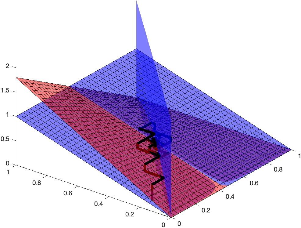
(a) k = 1.8

(b) k = 2.2
Figure 3: Cobweb plots of 3 dimensional orbits with initial conditions (0.1,0.2) for different values of k. The bottom plane corresponds to the regular xn,yn phase plane extended by yn+1 in the z direction
The varied behavior of such systems is observed in figure 3 where for smaller parameter values orbits decay to a fixed point while for larger values they expand into a stable orbit.
2.5 Bifurcations
These qualitative changes in the behavior of dynamical systems as a control parameter is varied are called bifurcations. In essence, bifurcations mark points where the system undergoes a transition from one type of behavior to another, such as from approaching a stable fixed point to periodic orbits or from periodic to chaotic motion. Bifurcations provide insight into the sensitivity of a system to changes in external conditions, and they are often characterized by dramatic shifts in the system’s dynamics [3].


(a) [2,4] (b) [3,4]
Figure 4: The bifurcation diagram for the logistic system also called the logistic map over the intervals [2,4] and [3,4]
A simple approach to tracking bifurcations is through graphing maps. For example, in the logistic equation xn+1 = kxn(1 − xn), varying k reveals how the system transitions from stable fixed points to oscillations and eventually to chaotic behavior [6]. A logistic map can be easily generated through a simple computer program that simulates the system for a wide array of parameter values and then selects a subset of the iterates and plots them against their parameter value. In this case for the logistic equation, the system was iterated 200 times and the final 50 points where sampled to produce figure 4. For parameter values less than 3 the system resolves quickly to a single point and then follows a 2 point orbit until the parameter comes to 3.5 where it once again doubles and so on until the chaotic behavior observed in figure 1 emerges. This behavior called a period doubling bifurcation, is one of the most common types of chaos1 in discrete dynamical systems [5]. Bifurcation diagrams are particularly useful because they can show us wrinkles in the behavior of the system. Presumably period doubling occurs uniformly and therefore covers the entire region evenly however seen in figure 3(b) that there is a pocket when the parameter k ≈ 3.85
1 In the 'ield of dynamical systems, chaos refers to systems with sensitive dependence on initial conditions colloquially referred to as the butter'ly effect
where orbits spread out. In fact there exists an entire family of third order stable orbits in this cavity [6].
3 Quantitative analysis
3.1 Fixed Points
The most prominent attributes of a dynamical system are its fixed points. In discrete systems, a fixed point is defined as a point x∗ , where the system’s transformation yields the same value: x∗ = g(x∗)
For example, in the time delay logistic equation fixed points are found by writing:
Solving this system of equations gives the solutions:
In a continuous system this manifests as a point where every derivative is zero: !$ !% = (($∗ ) = 0. An important classification on fixed points is their suitability. A fixed point is said to be stable if solutions with close initial conditions approach it as the system progresses forward through time and unstable if the inverse is true [3][9].
3.2 Linearization
3.2.1
Affine Dynamical Systems
Observing the dynamics of the simplest dynamical system; the affine, or linear, transformation where a and b are constants.
xn+1 = axn + b
Extending this transformation to a general expression:

The long term behavior of the system can be examined by taking the limit as n → ∞.

clearly if |a| < 1 then limn→∞ an = 0, meaning that orbits converge to a fixed point at b regardless of the initial condition of x. However, if |a| > 1 orbits will expand to infinity for any initial condition not x = b [9].
The continuous affine system:
! = ax + b
can be solved simply by rearranging terms and integrating to give the general solution where c1 is an arbitrary constant.

In this case taking the limit as t → ∞ all solutions diverge if a > 0 and conversely, converge if a < 0.
These forms precisely determine the behavior of any affine dynamical system for any time and at any initial condition. Crucially this form shows the stability of the fixed points in an arbitrary affine system. However, this kind of equation is impossible to write for systems with more complex dynamics and thus requires the development of techniques to approximate nonlinear systems as affine near equilibrium points. This is achieved by expanding the Taylor series of the transformation around a fixed point x∗ .

For points suitably close to x∗, the nonlinear terms reduce to zero due to the higher order powers of their terms. Thus, a linear approximation of the behavior of the system can be made which holds in a neighborhood {x ∈ ℝ | (x x∗) < r}.
F(xn) = F(x∗) + F ′(x∗)xn
and recalling our analysis in 3.1.1 the point is stable if |F ′(x∗)| < 1 and unstable if |F ′(x∗)| > 1. The same analytical approach can be applied to linearize continuous systems. The key difference is that, unlike discrete affine systems where stability depends on whether a value is less than or greater than 1, continuous systems use 0 as the threshold for determining convergence or divergence. In multidimensional systems, linearization again begins by expanding the system into its Taylor series around a fixed point and neglecting the higher-order nonlinear terms. This yields a linear approximation of the system near the equilibrium point: F(Xn) ≈ F(X ∗) + J(X ∗)Xn
where J(X ∗) is the Jacobian matrix of F evaluated at X ∗ .
This linear representation allows the behavior of points near the fixed point to be analyzed through the eigenvalues of the Jacobian matrix J(X ∗).
3.3 Finding Bifurcations
As discussed in section 3.2, bifurcations represent changes in the qualitative behavior of orbits in a dynamical system and further in section 3.3 orbits are intrinsically tied to the nature of the fixed
points in the phase space of the system. Therefore, by observing the nature of a linearized fixed point in relation to the system’s parameter values, bifurcations can be analyzed.
Considering the delay logistic equation with a fixed point at the point (1 ' ( ,1 − ' ( ). Computing the Jacobian matrix at this point:

with eigenvalues | λ | = √1 7 . When k > 2 the fixed point is unstable and for k < 2 the point is stable [5]. This matches with the behavior observed in the simulation in figure 4.
4 Invariant Manifold Theory
4.1 Separatrices
The exploration of invariant manifolds begins with the simplest case: separatrices in two-dimensional systems. Returning to the phase plane for the cooperative Lotka-Volterra system from section 2.3.
Figure 5: The phase plane for a continuous competitive system
In this system orbits seem to split into 4 sections depending on what section of phase space they begin from and progress towards. In figure 6 that these regions are split by a curve where orbits with initial conditions above expand to infinity and points below the line decay to the origin, and a curve that with time reversed, separates the trajectories flowing to the top left and bottom right corners. These lines called separatrices, are special trajectories in phase space that serve as boundaries between qualitatively different types of motion. These structures can be understood as a lower-dimensional example of invariant manifolds, which describe the long-term behavior of trajectories near fixed points. In simple systems, manifolds appear as seperatricies that divide phase space into regions with distinct dynamic behaviors either approaching fixed points, periodic orbits, or infinite expansion. In higher-dimensional and nonlinear systems, invariant manifolds serve the same role splitting phase space into regions of distinct behavior. A higher
dimensional invariant manifold need not be a line, it can be represented by a manifold of any dimension as it contains the behavior of every stable or unstable eigenvector.
4.1.1
Computing Separatrices
Given the Lotka-Volterra system in figure 6:

A saddle point was identified at (3/2,5/3). To compute the separatrices, the system is first translated so that this fixed point lies on the origin, this transformation yields the new system:

This new system has eigenvalues λ = ± √15 with eigenvectors

With these pieces in place, the computation of the separatrices can begin. The separatrix is first approximated as a power series:

, The derivative with respect to time is then taken for this series:

and by Substituting ! and % from the system and replacing the remaining y with the polynomial expression yields an equation that depends only on x. By considering points in a small neighborhood around the fixed point, similar to linearization, all terms with powers higher than a chosen n can be disregarded in the local neighborhood of the fixed point. So finally solving the resulting equation for the
coefficients ai gives us an approximation of the separatrix. Following this procedure for the third order approximation the following expression is obtained:


Solving for the coefficients gives 2 sets of solutions: , and ; and , and . These values for c line up with the fact that the separatrix is tangent to its associated eigenvectors at the fixed point since . Now by plugging these coefficients back into the polynomial gives the two seperatricies. Then by plotting these polynomials over the shifted system gives us the figure:

Figure 6: The phase plane for a the Lotka-Volterra system overlaid with the 9th order approximation of the stable (blue) and unstable (red) seperatricies
This was a simple approximation of a relatively straightforward system, yet it required a considerable amount of computation. As one might expect, separatrices become practically impossible to compute accurately in more complex systems. To address this issue, the concept of separatrices is generalized to invariant manifolds. [10].
4.2 Continuous Case
For continuous dynamical systems, a general nonlinear system takes the form where λ and µ are the linear parameters of the system and the functions h(x,y) and g(x,y) are the nonlinear terms of the system.:

This system is then rewritten in matrix form as $ = AX + γ(X)

where A is the Jacobian matrix at the fixed point: and γ contains the nonlinear terms.
To analyze the behavior near the fixed point, a solution of the following form is sought. X(t) = eAtξ(X)
Substituting this into the differential equation and simplifying leads to the following integral form where τ is an arbitrary initial time.

To understand the structure of the stable and unstable manifolds, a local neighborhood Q around the fixed point is defined: Q := {(x,y) : |x|,|y| ≤ r}, and within this neighborhood the local stable manifold is defined as the set of points remaining in Q under forward progression: 9 ) (:) = {! ∈ : | lim %→+ @ (A) ∈ : }
Similarly, the corresponding local unstable manifold consists of points that remain within Q under backward progression:
9 , (:) = {! ∈ : | lim %→+ @ (A ) ∈ : }
Therefore invariant manifolds correspond to solutions of the differential equations that remain bounded for all time, forwards in the stable case and backwards in the unstable case. To find each of these manifolds the general solution is projected onto the axes parallel to the stable and unstable eigenvectors respectively. The stable projection with τ = 0 is expressed as:

where πs is the projection matrix associated with the stable eigenvector. This projection corresponds to eigenvalues having negative real parts, so these terms decay over time. Ensuring that the stable manifold is bounded as t → ∞.
Contrastingly, the unstable projection corresponds to terms with positive real eigenvalues. Therefore, to fit our definition of an invariant manifold, a set of constraints must be found such that this projection remains bounded for all t. this projection can be rewritten as and since eAt → ∞ as t → ∞, for this solution to be bounded, a form must be found such that
Rearranging this expression leads to:

and since the choice of τ was arbitrary a change of variables τ = t can be performed to derive the unstable projection:

Using the linearity of these projections to combine the stable and unstable parts, X(t) = πsX(t) + πuX(t), the bounded solution to the differential equation is found:
At this point, the integral equation is reinterpreted as a new dynamical system, this time operating on functions instead of scalar states. The manifold equation is treated as a map on the space of trajectories, where each iteration refines the approximation of the invariant manifold.
The system was designed so that its solutions remain bounded for all t in a neighborhood of the fixed point. This property is crucial, as it allows the invocation of the Poincaré–Bendixson theorem, which insures the existence of a stable, attractive state within this bounded region of the function state. Using this fact in conjunction with Banach’s contraction mapping theorem requires that orbits in this bounded region approach the fixed point found from Poincaré–Bendixson.
To compute the invariant manifold in practice, the process begins with an initial guess for the trajectory functions such as a straight line or simple curve through the fixed point. These are plugged into the integral expression producing a new function, which is then fed back into the integral operator. This process yields better and better approximations of the manifold as the solution approaches the fixed point in function space. To visualize the manifold it is sufficient to chose any time t, it is usually most convenient to pick t = 0, and plot the parametric curve of x and y given by the initial condition σ [8].
4.2.1 Example:
Considering the nonlinear system given by the differential equations
! = 2x + xy – y2 ,
% = –y + x2 ,
with a fixed point at the origin. To approximate the invariant manifold near this point, begin by linearizing the system evaluating the Jacobian matrix A at the origin: ,

A has eigenvalues λ1 = 2 and λ2 = −1, indicating a saddle point with one stable and one unstable direction. Projecting solutions onto the eigenspaces, by defining the projection matrices: . allows for the decomposition of orbits into stable and unstable components. Using these projections to evaluate the integral found in 4.2 renders an operator T for the system, which acts on trajectories and approaches the invariant manifolds. In this case, the operator is given by , where σx and σy are initial parameters corresponding to the projection of the initial state. Starting from the zero function and taking σy = 0, the first iterate is


.
Inserting this back into the operator yields the second iterate:
Evaluating the integral and simplifying: produces the expression and evaluating at t = 0 gives the manifold approximation: ,


This shows the manifold as the graph of the function % = '! . or: .

Each successive iterate refines the approximation of the invariant manifold, with convergence guaranteed in a sufficiently small neighborhood of the origin. So continuing to the next iterate by feeding X2(t) into T again, generates polynomial corrections of the form:
4.3 Discrete Case
For discrete dynamical systems, consider a system of the form:

where λ and µ are the linear parameters of the system and the functions h(x,y) and g(x,y) are the nonlinear terms of the system. For discrete systems the local manifolds are expressed as the points in the neighborhood Q which remain inside Q under forwards and backwards iteration respectively. This is expressed similarly to the continuous case as: 9 ) (:) = {! ∈ : | lim / →+ C (/ ) (!) ∈ : } 9 , (: ) = {! ∈ : | lim / →+ C (/ ) (!) ∈ : }
To compute an approximation of the unstable manifold, it is written locally as a power series:
n = S(xn) = ∑ '2 !3 2 4 2 5.
That is, a function S(x) is sought such that the manifold consists of points of the form (xn,S(xn)). To ensure this manifold remains invariant under the transformation, the following invariance condition is imposed: yn+1 = S(xn+1) = ∑ '2 !36' 2 4 2 5.
Plugging S(xn) and S(xn+1) into the original system and rearranging, the following expression is derived.
By choosing the order of approximation and setting all terms !3 2 with i greater than the chosen order to zero, the coefficients υi can be solved for. This allows for the computation of an approximation of the manifold. [10].
Alternatively this expression solving the invariance condition can be interpreted as a power series solution of a dynamical system similar to the system T(x)(x) for the continuous case. In this view taking higher order approximations is analogous to iterating the system and since same conditions hold in this case as in the
continuous one, these solutions contract to the invariant manifold [12] [5].
4.4 Computation of Global Manifolds
Our analysis so far has only considered the local invariant manifolds in the region Q near the saddle point. The global manifolds consist of all points that eventually limit to the equilibrium in forward and backward time respectively. It is often necessary to find a larger representation of the manifold that can depicts the global behavior of the system. One way to analyze global development is by inferring the behavior of the manifold through broader knowledge of the system’s dynamics. For example, in the system considered in Figure 8, it is known that every orbit is bounded by the x and y-axes, and points in the bottom left corner are bounded by the stable manifold. Therefore the Poincare-Bendixson theorem applies, this theorem states that if an orbit is bounded in a region for all time it must approach either a fixed point or a stable orbit in this region. From this, it can be inferred that the unstable manifold must approach some fixed point or stable orbit in this region. Since the origin is a fixed point in this region, it can be concluded that the separatrix approaches the origin. The Poincare-Bendixson theorem is one of the most consequential theorems for the qualitative analysis of dynamical systems, however it is limited to only two and lower dimensional continuous systems. To overcome this limitation several computational models have been developed to numerically compute the global manifolds. Two notable computational approaches are a subdivision algorithm by Dellnitz and Hohmann, and a geodesic level set method developed by Krauskopf and Osinga.
4.4.1 Subdivision Method
Dellnitz and Hohmann developed a subdivision algorithm aimed at approximating global attractors, which inherently contain all
invariant sets. The global attractor of a system is defined to be the set which is eventually approached by every orbit in a region of the underlying dynamical system. In other words it contains all the possible end states of the system. In particular, the global attractor contains all the limit sets including the unstable manifold. The core idea Dellnitz and Hohmann’s method is to iteratively refine a covering of the phase space to capture the structure of these manifolds.


(a) (b)
Figure 7: (a) A series of subdivisions for the 3 dimensional

dynamical system and (b) the final approximation of the manifold [4]
The algorithm begins by enclosing the region of interest in a finite collection of compact sets, which can be thought of as simple geometric shapes like boxes. Each set is then tested to determine if it intersects the global attractor. This is typically done using a combination of forward and backward time integration to check for invariant behavior within the set. Sets that do not intersect the attractor are disregarded while sets that intersect the attractor are subdivided into smaller subsets, and the process is repeated. Through successive iterations, the collection of sets converges to a detailed approximation of the global attractor and its unstable manifolds. This method is particularly advantageous because it
provides a systematic way to handle high-dimensional systems and can prove the existence of certain dynamical features within the attractor. [4]
4.4.2 Geodesic Level Set Expansion
Krauskopf and Osinga introduced a method that computes global manifolds by constructing geodesic level sets. This approach focuses on the intrinsic geometry of the manifolds, treating them as surfaces of constant geodesic distance from a reference point on the manifold.
The process starts with a local approximation of the manifold near an equilibrium point or periodic orbit like that computed in 4.2. From this initial segment, the method extends the manifold by incrementally adding points that are a fixed geodesic distance away from the existing manifold. This is achieved by solving boundary value problems (a special kind of differential equation) to ensure the new points adhere to the dynamics of the system.

Figure 8: The computed global manifold for the Lorenz system. The alternating colored bands represent each distinct topological circle computed [7].
By iterating this procedure, the algorithm traces out the manifold globally, capturing its intricate structure. One of the strengths of this method is its ability to handle manifolds with complex geometries, including folds and twists, by focusing on their intrinsic distances rather than extrinsic coordinates. [7]
Both methods have significantly advanced the numerical computation of global manifolds in dynamical systems, providing researchers with powerful tools to explore and understand complex behaviors in various applications.
4.5 Applications of Invariant Manifold Theory
One modern application of invariant manifolds is in the analysis of the pituitary system. The pituitary gland is a small but critical organ located at the base of the brain. It regulates a wide array of physiological processes by secreting hormones that control growth, metabolism, stress response, and reproductive function. It does so by receiving electrical signals from the hypothalamus. The strength and pattern of these electric signals determine the type and amount of hormones that are released by the pituitary. One such signal is a patter called bursting.

Figure 9: An example of a bursting cycle from a rat pituitary gland [11].
Bursting is a rhythmic pattern of electrical activity in which a cell alternates between periods of rapid active potentials (spiking) and silent phases. This oscillatory behavior is fundamental for hormone secretion in the pituitary. The bursting pattern directly influences the timing and amount of hormone release, ensuring that endocrine signals remain effective and properly regulated. The bursts arise due to the interaction between fast and slow ionic processes in the cell
membrane due to sodium and potassium, and calcium respectively. By modeling the interactions between these compounds and the resultant pituitary activity Stern et al. were able to analyze the dynamics of the system to better understand the chemical processes that regulate the endocrine system [1].
Dynamically the system divides into a fast subsystem that determines the spikes of the bursting pattern and a slow calcium subsystem that drives the pattern. Because of this the researchers were able to focus in on the slow subsystem as it determines the general dynamics of the system. This subsystem was shown to contain a the active and silent phases were identified by high-voltage and low-voltage states respectively [1].
Phase resetting refers to how a periodic biological system such as the bursting activity of pituitary cells responds to an external perturbation. In this context, a perturbation can be a stimulus such as an injected current, a neurotransmitter signal, or another form of external input. Depending on when the perturbation occurs during a burst cycle as well as the strength of the input, it can either advance, delay, or completely displace the timing of the next burst.
This concept is crucial for understanding how pituitary cells synchronize with physiological signals, ensuring precise hormone release. Phase resetting is often studied using Phase Response Curves (PRCs), which describe how a system’s cycle shifts in response to external perturbations.

Figure 10: Fast subsystem bifurcation diagrams and superimposed periodic orbits for various perturbations from a study of inner ear sensory cells whose development depends on a similar system to hormone release in the pituitary. The blue solid and the red dashed curves represent the stable and unstable equilibria, respectively. The blue and green surfaces represent the stable and unstable periodic orbits, respectively [2]
If a perturbation occurs at the right phase as seen in (a), (b), and (c), it attains the high-voltage state and synchronizes with the natural cycle of hormone secretion. However, if perturbations happen during the wrong phases, they can desynchronize bursts as in (e), (f), and (g). In these examples the perturbation misses the high-voltage state and cycle back to low voltage without initiating hormone secretion.
In a healthy pituitary gland, the natural ionic interactions produce the proper charge structures in order to self regulate the endocrine system. However if there exists a defect in the gland this can cause improper hormone regulation that can cause endocrine disorders that have crippling effects on development. In such cases, the pituitary can be regulated externally through the use of medications. These medications serve as external perturbations and as the bursting cycle of the pituitary is very precise the perturbation must be exactly timed to induce the desired hormone secretion. By modeling phase resetting mathematically using invariant manifolds, researchers can simulate how external stimuli affect hormone secretion dynamics. The ability to predict how a burst will reset helps in designing interventions for hormonal imbalances [11].
5 Conclusion
This thesis explored the geometric structures that govern the evolution of nonlinear dynamical systems. In cases where analytic solutions are impossible, the topology of phase space becomes the focus of analysis. In particular, invariant manifolds offer a powerful method of studying the behavior of a system, not by tracking single trajectories, but by analyzing the structures that constrain and guide all possible motion. Through the use of computational techniques applied to both discrete and continuous systems, these manifolds can be approximated and visualized beyond their local neighborhoods. The result is a clear understanding of the local rules that generate complex global structures, and how these structures, in turn, shape the full dynamical landscape [5] [12].
A striking consequences of global manifold theory is the appearance of heteroclinic intersections. These are points which appear where the stable and unstable manifolds of two distinct fixed points intersect.

Figure 11: A heteroclinical intersection between manifolds emanating from the fixed points p and q
Since this intersection point lies on the a stable manifold the next intersection must also lie on that manifold. However this point also lies on the unstable manifold of a different fixed point so the next iteration also lies on this manifold. Therefore the manifolds must intersect a second time an the a third and so on approaching the fixed point of the stable manifold. As the manifold gets closer and closer to this fixed point it is pulled apart by the other unstable manifold so that it is compacted in one direction by the stable manifold and stretched in the other by the unstable one. The same argument can be made with time reversed to show that the stable manifold is also stretched and compacted near the other fixed point resulting is the picture seen in figure 12. This leads to extraordinary chaotic behavior. In fact it can be shown that if points that visit the neighborhood of p are called heads and points near q tails, then for any random sequence of coin flips, there exists an orbit in the dynamical system that realizes exactly this sequence of results. This reveals that the system is capable of encoding arbitrary symbolic
dynamics within its orbits. These orbits are not only chaotic but also deterministic; there must exist an orbit satisfying this condition for ANY sequence [12]. This behavior is present more generally in horseshoe maps where entire regions of phase space are contorted resulting in an infinite web of heteroclinical intersections. These intersections mark the onset of deterministic chaos and signal the transition from the relatively smooth behavior simple systems to the intricate, layered complexity of complicated modern applications. From fluid flows to celestial mechanics, this underlying geometric scaffold reveals a deep structure behind seemingly erratic systems [5].
Invariant manifolds are not merely a tools for approximation, but a window into the deeper structure of complex systems. By analyzing how manifolds emerge, intersect, and evolve, a broader understanding of both predictable and chaotic behavior becomes possible. As computational tools continue to advance, so too will our ability to uncover and manipulate the invisible geometry of complex systems’ geometry that ultimately governs everything from planetary orbits to neuronal firing patterns.
References
[1] Computing Global Invariant Manifolds: Techniques and Applications, 10 2014.
[2] H. Baldemir, D. Avitabile, and K. Tsaneva-Atanasova, Fast subsystem bifurcation diagrams and superimposed periodic orbits, 08 2019.
[3] P. Blanchard, R. L. Devaney, and G. R. Hall, Differential Equations, Brooks/Cole, Cengage Learning, 4 ed., 2012.
[4] M. Dellnitz and A. Hohmann, A subdivision algorithm for the computation of unstable manifolds and global attractors, Numerische Mathematik, 75 (1997), pp. 293–317.
[5] R. Devaney, A First Course In Chaotic Dynamical Systems: theory and experiment, CRC Press, 04 2020.
[6] R. Gilmore and M. Lefranc, Discrete Dynamical Systems: Maps, The Topology of Chaos, John Wiley & Sons, 09 2012.
[7] B. Krauskopf and H. M. Osinga, Computing geodesic level sets on global (un)stable manifolds of vector fields, SIAM Journal on Applied Dynamical Systems, 2 (2003), pp. 546–569.
[8] J. D. Meiss, Invariant Manifolds, Differential Dynamical Systems, Revised Edition, SIAM, 01 2017.
[9] P. J. Olver, Nonlinear systems, University of Minnesota, (2022).
[10] R. H. Rand and D. Armbruster, Perturbation Methods, Bifurcation Theory and Computer Algebra, Springer-Verlag, 1987.
[11] J. V. Stern, H. M. Osinga, A. LeBeau, and A. Sherman, Resetting behavior in a model of bursting in secretory pituitary
cells: Distinguishing plateaus from pseudo-plateaus, Bulletin of Mathematical Biology, 70 (2007), pp. 68–88.
[12] E. Zehnder, Lectures on Dynamical Systems, European Mathematical Society, 2010.