
Abstract
This work presents results on AutomataGPT, a small transformer model designed to predict how 2D binary CA evolve and infer their rules from one step. AutomataGPT was trained on three different scales, 2 rules, 10 rules, or 100 rules. After training, AutomataGPA’s ability to solve the forward problem can be tested, i.e. predicting the next grid, and the inverse problem, i.e. predicting the ruleset. The findings of this paper suggest that training on a broad set of rules yields a much higher accuracy for both the forward and inverse problem, showing that the model can generalize beyond a single CA. This allows researchers to use CA as a framework for real-world modeling, with AI figuring out discrete local update rules from CA simulations of real-world phenomena.
Introduction
Imagine a 16x16 grid that is projected onto a torus, or a donut. Each square is either “on” (1) or “off” (0). At every timestep, the program looks at each square’s neighbors to decide whether it should stay on or switch off. This mechanism, where a cell’s fate is determined by its local interactions, defines a class of mathematical objects called cellular automata (CA). Despite the simple instructions of CA, they frequently display extremely intricate behaviors. This leads to a certain paradox, in which complex patterns arise from simple interactions between neighboring cells. Stephen Wolfram, in his seminal work A New
Kind of Science, 1 showed that rules that rely only on local neighborhoods can produce global patterns ranging from stable structures of 1s to entirely random configurations. Traditional mathematical and probabilistic methods struggle to capture the nuances of the supposedly random configurations of cellular automata.
The primary draw of studying CA is because CA are able to model a wide variety of biological and mathematical processes. For example, CA are used in the study of the spread of forest fires, with cells turning “on” if fire spreads into that area;2 another CA might capture how traffic jams form and dissolve on a highway;3 yet another can track how cells multiply in a model tissue sample. Some CA are Turing-complete, meaning that, in principle, they can perform all the computations a standard computer can if given the right rules.4 The ruleset for each CA can be defined as being the collection of rules that govern how a given cell locally moves from one state to another. For a binary CA, each neighborhood arrangement can map to either 0 or 1 at the next time step. If one knows the exact rules of a CA, it is straightforward to evolve the CA step-by-step. However, one can imagine a scenario in which there is a sample of the grid at two states, the “before” and “after” states. Can the local rules of the CA be inferred from these samples? This becomes difficult when
1 Stephen Wolfram, A New Kind of Science (Champaign, IL: Wolfram Media, 2002).
2 Feng, Tianjun, Keyi Liu, and Chunyan Liang. "An Improved Cellular Automata Traffic Flow Model Considering Driving Styles." Sustainability 15, no. 2 (2023): 952. https://doi.org/10.3390/su15020952
3 Freire, J. G., and C. C. DaCamara. "Using Cellular Automata to Simulate Wildfire Propagation and to Assist in Fire Management." Natural Hazards and Earth System Sciences 19, no. 1 (2019): 169–179. https://doi.org/10.5194/nhess-19-169-2019.
4 John von Neumann, Theory of Self-Reproducing Automata, ed. and completed by Arthur W. Burks (Urbana: University of Illinois Press, 1966).
one considers that the most basic type of CA has 218 possible rulesets. This is one of the simplest types of CA - the CA that are used in real-world mathematical modeling can have trillions of possible rulesets. A random search is unwieldy, so artificial intelligence can be used to find rules based on two states. Transformers are a type of artificial intelligence. They were first used in natural language processing, where they were used to read text to predict the next token in a sentence.5 Transformers used self-attention mechanisms to process long sequences.6 This same method can be used to learn the rules of any data with a sequential pattern, such as CA grids flattened into tokens. Can one model handle multiple rules instead of memorizing a single one, and can it solve the inverse problem from a single step of state evolution?
Research Question
This project aims to address the following questions: Can a small, decoder-only transformer model accurately learn both the forward (forecasting the next 2D grid state) and inverse (inferring the rule matrix) tasks for binary cellular automata, and how does expanding the set of training rules affect performance on these tasks?Can training on a small set of unique rules (2 or 10) yields a higher or lower accuracy to training on a larger set of unique rules (100)? And finally, can the model’s performance rise enough to make it a general CA simulator?
5 Vaswani, Ashish, Noam Shazeer, Niki Parmar, Jakob Uszkoreit, Llion Jones, Aidan N. Gomez, Łukasz Kaiser, and Illia Polosukhin. "Attention Is All You Need." Advances in Neural Information Processing Systems 30 (2017): 5998-6008.
6 Ashish Vaswani et al., “Attention Is All You Need,” in Advances in Neural Information Processing Systems 30 (2017): 5998–6008.
Methods
Training Process
AutomataGPT-2DBD was created in Python and built with the software library x-transformers.7 It was trained on a powerful computer equipped with a high-performance graphics card, the NVIDIA RTX A4000. Hyperparameters were optimized to make the model run efficiently based on the capabilities of the graphics card. The graphics card has 16 GB of memory. Each training iteration is a small step in teaching a model how to update the tiles on the grid. At every step, the model takes an initial pattern and tries to predict the next pattern using the given rules. After each guess, the model’s internal settings were adjusted so it can predict more accurately next time. Over many such steps, or iterations, the model refines its understanding and learns to produce the correct updates to the grid. At each iteration, the model’s performance is recorded by computing both training and validation losses. Training loss reflects how well the model fits the data it learns from directly, while validation loss shows whether the model is capturing more general patterns rather than memorizing specific examples. Every epoch, the model’s accuracy on predicting the next grid state is assessed across all samples in the testing dataset. Since the next state involves 256 positions for a 16×16 grid, accuracy is defined as the fraction of those 256 positions predicted correctly. By monitoring how both loss values and accuracy scores change over time, the model’s predictions were analyzed when they became stable and reliable.
7 Phil Wang. "x-transformers: A Concise but Complete Full-Attention Transformer with a Set of Promising Experimental Features from Various Papers." GitHub repository. Accessed March 9, 2025. https://github.com/lucidrains/x-transformers.
Database
The dataset includes a wide variety of two-dimensional binary cellular automata samples. Each sample consists of a rule matrix that encodes all possible neighborhood configurations (18 total) and their corresponding next states (2 possible states), resulting in 36 bits of information. Each of these 18 configurations can lead to either a 0 or a 1, and since there are 218 possible deterministic rules, the dataset is incredibly diverse. An initial condition (IC), which is a 16×16 grid of binary states (256 bits). The next state (GS2), which is the correct 16x16 configuration that follows from applying the rules from the rule matrix to the IC. The entire dataset is split such that 90% of samples are used for training the model’s parameters, 9% for validation (to adjust the model and fine-tune the training without overfitting the model), and 1% for testing (to confirm the generalization the rules the automata learned). To make these patterns easier for the model to process, both the IC and the GS2 can be represented as one-dimensional sequences of length 256, each element being either 0 or 1; this is because each IC and GS2 is a 16x16 grid. The rules, represented as a 2x18 binary matrix, may be flattened into 18 tokens. A token represents the next state of a given configuration of cells. The rules, the IC, and the GS2 were concatenated together into a single linear sequence. This consistent format allows the transformer to understand the twodimensional mathematical patterns as a one-dimensional string.
Rules Matrix Generation
As shown in Figure 1, the transformation from a graph to a 2D binary adjacency matrix illustrates the mapping from neighborhood configurations to cell state transitions. Each rule matrix is randomly generated. To do this, the net possible rules of
the rule matrix must first be rigorously derived. Consider each cell on the grid along with its eight neighbors, forming a local 3x3 neighborhood. In a binary automaton, each neighbor is either 0 or 1. For a cell’s own state, there are 2 possibilities. Hence, there are 18 unique neighborhood configurations. Because each cell has 2 possible future states (0 and 1), the number of rule matrices can be represented as a 2x18 grid. The rows of the grid are the possible next states of that cell, and the columns represent each neighborhood configuration. Hence, there are 218 possible grids.

Figure 1: Transformation of a graph representation of state transition in 2D binary CA to a 2D binary adjacency matrix. The latter mathematical object is referred to as a rule matrix. One can see how the value in top column represents the probability that the next state of a given cell with the metastate represented by the image in the top row evolves into a dead cell.
Initial Condition Generation
Initial conditions of each automaton are generated by an algorithm. Note that each tile can be either “off” (0) or “on” (1). To decide how likely a tile is to be off or on, pick one random number between zero and one; this number can be called “p.” If there are only 2 states, 0 and 1, then the probability that a tile is off is p and the probability that a tile is on is 1-p. For example, if p is 0.3, that means each tile has a 30% chance of being off and a 70% chance of being on. After "p" has been chosen, the state of each of the 256 tiles is set. For each tile, another random number, n, is selected from the interval between zero and one. If n is greater than p, the tile is set to off (0); otherwise, it is set to on (1).
The goal of this convoluted generation process is to ensure that the dataset is broad-entropy, ie. the ratio of 0’s and 1’s in each automaton ranges equally from 0% to 100%, rather than a binomial distribution around 50%. If each cell was assigned with a 50% probability of equalling 0 or 1, then the dataset would not be truly representative of real-world conditions.
NGS Generation
Once the model receives a rules matrix (which encodes all possible state transitions for a binary, two-dimensional cellular automaton) and an initial condition (IC), the next logical step is to determine the subsequent game state, here called “NGS” or next game state. Each automaton has 256 cells, each of which may be equal to 0 or 1. By examining the neighborhood configuration of each cell, the code can find the column in the rule matrix that corresponds to the neighborhood configuration of that cell. The rules matrix tells us whether the cell should become 0 or 1 in the
next time-step. The code can apply this process to each of the 256 cells simultaneously, producing the next 16×16 grid. This fully updated grid is the NGS. Generating the NGS from the IC and rules is a deterministic procedure: the same IC and rules will always create the exact same NGS, guaranteeing a direct one-toone mapping that the model will learn.
Instruction Tuning
Instruction tuning is a method to guide the model’s training process by embedding the problem description and desired output format directly into the input data. Instead of simply providing the raw sequences of tokens representing the rules matrix, IC, and NGS, the dataset is formatted into prompts that clearly state what the model must do. For example, a prompt might say: “Predict the next state given the initial condition and the rules,” and then show the rules and the IC, marking where the NGS should be placed by the model. Certain tokens and textual clues will help the model understand where each NGS should be placed. This formatting instructs the model to actually produce a transform to verify its knowledge instead of just learning patterns.
Data Splitting
To properly train and evaluate the model, the dataset is divided into three subsets: training, validation, and testing. Approximately 90% of the samples become the training set. This is the dataset subset the model sees repeatedly while adjusting its internal parameters (weights) through gradient-based optimization. About 9% of the samples form the validation set, which is used to monitor the model’s performance without directly updating the model’s weights from these samples. By examining validation loss (and possibly other metrics), researchers can detect overfitting (where the model memorizes
training examples but fails to understand the patterns behind the examples) or confirm that training is progressing as intended. 1% of the samples constitute the testing set. This small portion is held out until training is completely finished. Only then is the model’s accuracy on this unseen data evaluated, ensuring a reliable measure of the model’s true generalization performance. By separating the data, researchers can understand whether the model truly understands the rules that govern cellular automata or whether it has simply memorized the entire dataset.
Tokenization
Tokenization is the process of encoding complex data as ‘tokens.’ A limited alphabet of 22 tokens is first defined. Tokens represent binary digits, or a symbol that represents the start and end of a section. This way, the model only needs to handle a small set of symbols. Then, two-dimensional 16-by-16 grids (which has 256 cells), are turned into a single row of 256 binary values. Each binary value (0 or 1) is turned into a token from our small set of tokens. Similarly, the rules can be flattened into a 1d list of 18 tokens. The program then concatenates the rules, the initial condition, and a placeholder for the next state into a single sequence.
Inference
Inferences were performed in both forward and inverse modes to evaluate and validate model predictions under minimal prior assumptions. The procedure consisted of generating outputs from a pretrained model and comparing these outputs to the true outputs, either in the form of binary strings or rule matrices. The core methods are outlined below.
Forward Problem
Forward inference was conducted by systematically iterating over the testing dataset and extracting the initial conditions (IC) and corresponding rules matrices (RM) for each sample. These elements were tokenized and provided as input to the AutomataGPT-2DBD model, which then auto-regressively generated the inferred next game state (GS2) with the temperature parameter set to zero, ensuring deterministic output. The generated GS2 was subsequently decoded into a binary string, isolating only the relevant binary data (0s and 1s) for comparison with the ground truth. A custom accuracy computation procedure was employed to measure the correspondence between the predicted GS2 and the actual GS2, resulting in an accuracy score for each individual sample. These per-sample accuracy scores were systematically logged, and an overall average forward accuracy was calculated across all testing samples.
Inverse Problem
Inverse inference was conducted to reconstruct the rules matrix (RM) governing a cellular automaton from observed initial conditions (IC) and subsequent game states (GS2). For each sample in the testing set, the IC and GS2 were extracted and tokenized before being input into the AutomataGPT-2DBD model. The model then auto-regressively generated an inferred RM with the temperature parameter set to zero to ensure deterministic output, which was subsequently decoded and reshaped into a 2×18 array representing the binary state transitions.
The inferred RM underwent a validation process to ensure its plausibility by verifying that each column's entries summed to one, confirming valid transition probabilities. If an inferred RM
failed this validation, both accuracy metrics, Rules Matrix
Inference Accuracy (A_RMI) and Inferred Rules Matrix
Application Accuracy (A_IRMA), were assigned a value of zero for that sample. For validated RMs, the IC was updated using the inferred RM to generate a computed GS2, which was then compared to the ground truth GS2 to calculate A_IRMA. If the computed GS2 perfectly matched the ground truth, A_RMI was set to one; otherwise, it was determined by the proportion of correctly inferred tokens relative to the total number of tokens in the RM. Both A_RMI and A_IRMA were recorded for each sample, and average inverse problem accuracies were computed across the entire testing set.
Results and Discussion
Forward Problem Quantitative Results
Accuracy in predicting the next 16x16 grid increases with the number of rule matrices (N_RM) in the training set. For N_RM=2, the average accuracy on the testing set is 63.0 percent. For N_RM=10, accuracy improves to 81.4 percent. At N_RM=100, accuracy reaches 98.5 percent, with only 3 out of 200 samples deviating from a perfect match. The fraction of perfectly predicted samples (f_p) stands at 10.5 percent for the 2rule model, 58.5 percent for the 10-rule model, and 98.5 percent for the 100-rule model. These results show a substantial drop in error as the training set expands across more distinct rules.
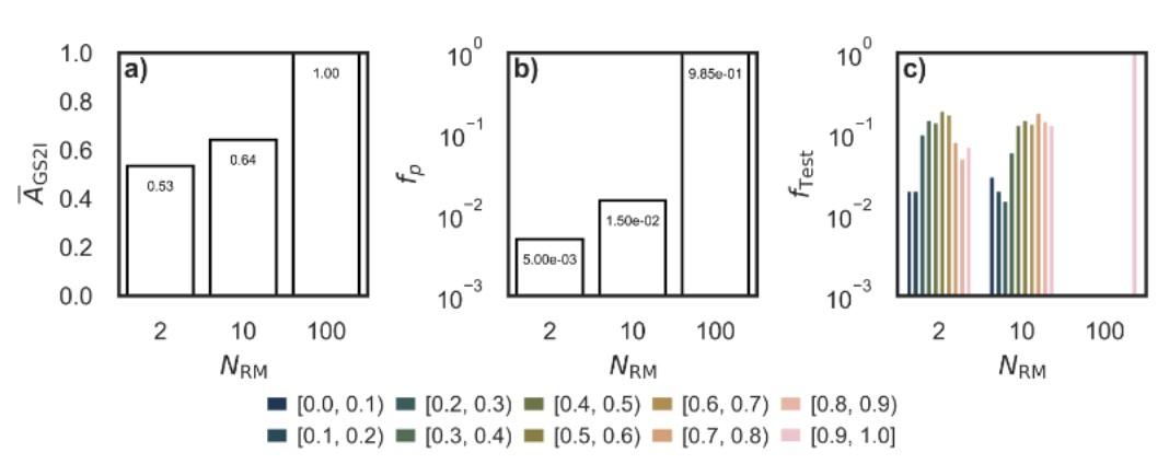
Figure 2: The first graph shows the correlation between the N_RM and the accuracy of the forward problem. At N_RM=2, A_GS2=0.53, at N_RM=10, A_GS2=0.64, at. N_RM=100, A_GS2=1.00. The second graph shows the correlation between N_RM and f_p (the percentage of samples that were predicted perfectly). At N_RM=2, f_p=0.5%, at N_RM=10, f_p=1.5%, but at N=100, f_p shoots up to 98.5%. The third graph is a more in-depth version of the second graph, such that shades of darker blue are equivalent to a very low accuracy and lighter shades of pink are equivalent to a very high accuracy.
Inverse Problem Results
The model’s ability to reconstruct the rule matrix is quantified by its average Rules Matrix Inference Accuracy (A_RMI). With N_RM=2, A_RMI is 0.60, with about 10 percent of the inferred matrices deemed illogical. When N_RM=10, A_RMI increases to 0.77, and illogical outputs drop to 6 percent. At N_RM=100, A_RMI reaches 0.92, while illogical outputs fall below 1 percent. For Inferred Rules Matrix Application Accuracy (A_IRMA), the 2rule model scores 0.68, the 10-rule model 0.84, and the 100-rule model 0.95. Perfectly reconstructed rule matrices rise from under 5 percent for 2 rules to almost 50 percent for 100 rules (Figure 2).
Comparative Analysis of Forward and Inverse Problems
Forward prediction requires applying a known rule matrix once to obtain the next grid. By contrast, the inverse task demands extracting every transition from a single observed outcome. At lower N_RM values, forward accuracy is notably higher than inverse accuracy. With just 2 rules, forward predictions reach 63.0 percent while rule inference lags behind. By N_RM=100, both tasks show high performance. This contrast indicates that estimating a complete set of transitions is more challenging than performing a single update, although more diverse training is able to bridge the gap.
Performance Across the Rule Space
As the model sees a wider variety of rules, it handles novel or “distant” samples more effectively. At N_RM=2, test samples whose ground truth rule matrix differs sharply from the training examples often produce lower accuracy. Expanding to N_RM=100 broadens coverage, making it likely that any given test rule matrix is either already seen or at least similar to a seen one. Due to this, the correlation between distance and accuracy diminishes. This implies that a high-entropy sampling of the possible transitions allows for a better generalization of both predicting grids and inferring the rule matrix.
To quantify how well the model generalizes with increasingN_RM , c dissimilarity tests can be used to figure out how close to the true rule matrix the solution to the inverse problem is. The first test is the Hamming Distance. Imagine there are two strings of 0s and 1s, one representing the true rule matrix, and the other representing the predicted rule matrix. The Hamming distance counts how many positions differ between the two strings. If the rule matrices are represented as simple strings
of 18 binary digits, a low Hamming distance means the rules are nearly identical; a high distance means many of the rules differ. The second test is the Jaccard distance, which compares the number of common features between sets with the total number of features. The third test is the Jensen-Shannon Divergence, which measures the difference between two probability distributions. This measures how similar or different the actual distributions of values are between the true rule matrix and the predicted rule matrix.
One can compute the average distance, D_RM, between the rule matrix of the test sample and the two most similar rule matrices in our training set. The dissimilarity of the two most similar rule matrices can then be compared in the training set and the dissimilarity of the true rule matrix and the most similar rule matrix in the training set. Essentially, calculating these distances measures whether the rule matrix in the validation set is similar to a rule matrix that the model has been trained on. When a rule matrix in the validation set is very similar to those the model saw during training, one would expect a high accuracy. When they are very different, one might expect a lower accuracy.
The experimental results clearly show that when the model is trained with N_RM=2, the model poorly performs both the forward and inverse problems when D_RM is high. However, the model N_RM=2 performs significantly better when D_RM is low. This is because when D_RM is high, the rule matrix in the validation set is incredibly different from the rule matrices in the test set.
Interpretation
The results of this work show that AutomataGPT is able to learn and apply CA rules with very high accuracy. As the training
set expands to include a broader range of rules, the forward prediction of the next grid state becomes nearly perfect. The inverse problem reveals that even when the inferred rule matrix deviates from the correct rule matrix, AutomatGPT is still able to produce the correct grid update, likely due to the fact that the incorrect parts of the rule matrix not being applicable to that particular NGS. The transformer model is able to find robust token relationships that generalize very well across unseen rule matrices. In short, the model is able to almost completely understand CA rules using just a tiny fraction of the trillions of possible initial conditions.
Conclusion and Future Work
This work shows that a small, decoder-only transformer can learn and apply CA rules with high accuracy. The model achieves near-perfect forward and inverse prediction. The use of explicit rule matrices provides an abstract generalization of CA to real-world systems. Future work will extend this framework to nstate stochastic cellular automata. The current study focused on deterministic, binary systems. In contrast, stochastic cellular automata have randomness in their evolution; the next state is taken from a probability distribution rather than being fixed by the rules.
Future work will extend this framework to n-state stochastic cellular automata. The current study focused on deterministic, binary systems. By abstracting the rule matrix, the AutomatGPT can simulate any kind of cellular automata, including those with multiple states and inherent randomness. This is important due to the fact that many real-world systems are inherently random. For example, if one is using a cellular automaton to predict what will be built in an area with mixed-use
zoning, it could be an apartment building, a single-family home, a shop, or any number of different buildings. There are a very large number of factors that are impossible to isolate in a cellular automaton, such as zoning and planning commission approval.
We plan to use this future model, trained on stochastic cellular automata, to predict the growth of rhizomorphs. Rhizomorphs are essentially a variety of fungus. The growth of rhizomorphs is not well-understood, there are no existing mathematical models that are able to consistently predict how rhizomorphs grow. We plan to take videos of thousands of growing rhizomorphs in a variety of different soil conditions, then use existing machine learning techniques to isolate the rhizomorphs in the video against the background. This will give us a video of white pixels on a black background that represent the growth of the rhizomorphs. Then, the white pixels can be labeled as “alive” cells and the black pixels can be labeled as “dead” cells in a cellular automata. We can then use a stochastic version of AutomataGPT that is able to solve the inverse problem of these rhizomorph CA. This will give us a stochastic cellular automaton model that can simulate the growth of rhizomorphs given an initial state.
Bibliography
Wolfram, Stephen. A New Kind of Science. Champaign, IL: Wolfram Media, 2002.
Feng, Tianjun, Keyi Liu, and Chunyan Liang. "An Improved Cellular Automata Traffic Flow Model Considering Driving Styles." Sustainability 15, no. 2 (2023): 952. https://doi.org/10.3390/su15020952.
Freire, J. G., and C. C. DaCamara. "Using Cellular Automata to Simulate Wildfire Propagation and to Assist in Fire Management." Natural Hazards and Earth System Sciences 19, no. 1 (2019): 169–179. https://doi.org/10.5194/nhess-19-169-2019.
von Neumann, John. Theory of Self-Reproducing Automata. Edited and completed by Arthur W. Burks. Urbana: University of Illinois Press, 1966.
Vaswani, Ashish, Noam Shazeer, Niki Parmar, Jakob Uszkoreit, Llion Jones, Aidan N. Gomez, Łukasz Kaiser, and Illia Polosukhin. "Attention Is All You Need." Advances in Neural Information Processing Systems 30 (2017): 5998–6008.
Wang, Phil. "x-transformers: A Concise but Complete FullAttention Transformer with a Set of Promising Experimental Features from Various Papers." GitHub repository. Accessed March 9, 2025. https://github.com/lucidrains/x-transformers.