Isabella Silvestrini Zorrilla
Senior Thesis | 2025

Modeling Long-term Habitability in Known Exoplanets
Isabella Silvestrini Zorrilla
April 2025
Modeling Long-Term Habitability in Known Exoplanets
Isabella Silvestrini Zorrilla
April 11, 2025
Introduction & Background Information
Star Luminosity & Habitable Zones
Many researchers in astrobiology have been interested in habitable exoplanets since they were first discovered in 1994. In order to tackle the problem of finding habitable exoplanets, we must first define habitability. Since we cannot visit other planets, we assume a universality of known physical laws and define habitability as the minimum conditions required to sustain life on Earth. Instantaneous habitability refers to those conditions (defined below) being present in a planet for a relatively short and/or infinitely small period of time. Long-term habitability is defined as the sustained habitability of a planet long enough for intelligent life to develop.
In order for life to develop, three conditions have to be met: energy, nourishment, and water. One is energy. Most complex organisms can derive it from the sun, but some singlecelled organisms can derive their energy from chemicals in their environment. Second, all organisms need some sort of nourishment in order to survive. On Earth, all living things derive their energy from six different elements which are present in most exoplanets: Iron, Calcium, Phosphorus, Potassium, Sodium, and Magnesium. Some researchers theorize that an imbalance in Methane might indicate a sign of life, because it is a natural byproduct of carbon based organisms. In order to determine whether a planet meets the chemical requirements for life, scientists use we have to use a method called spectroscopy. By measuring the absorption lines of a
planet, from its star’s emission spectrum, we can detect some elements and molecules in the atmosphere. However, this is a very difficult process, and is impossible for most known planets.
Lastly, living things need liquid water to survive. Because the first two requirements are either almost always present (Energy) or very hard to detect (Atmospheric components), we use the possibility of the existence of liquid water as the primary factor in determining habitability. A planet’s habitable zone (HZ) is the distance from its star, where the conditions are just right to support liquid water. If the star is too close to the sun, the water evaporates; Too far, and the water will freeze into ice. This is why this HZ is often called the “Goldilocks Zone.” Put simply, to calculate the distance where the habitable zone lies in a main sequence star, we must take the absolute luminosity of the star and apply it to the formula for the inner and outer radii of a star’s HZ, (Kasting et. al., 1993) (Whitmear et. al.,1996): ()

Where ri and ro are the inner and outer boundaries for the HZ respectively. Lstar is the absolute luminosity of the star, meaning the intensity of the thermal radiation of the star time the surface area:
L = 4πR2starσT4star
Where Rstar is the star’s radius, T is the temperature in Kelvin, and σ is the Stefan Boltzmann constant (5.67E-8 W · m 2 · K 4). 1.1 and 0.53 are the constant values representing the stellar flux at the inner and outer radii, respectively (). A star’s Stellar flux (also known as bolometric flux) is the Luminosity over a specific area. It obeys the inverse square law, which means the flux decreases
quadratically as you increase the distance from a star. It is given by the equation
Fbol = Lπd2
Where L is the luminosity, and d is the distance from the star to the object.
However, there are a few important points that should be noted about the Habitable Zone concept. One is that it only describes the area where liquid water can exist at the surface. Stellar objects outside of the HZ may have liquid water beneath their surface. One such object is Saturn’s largest moon, Titan, which has liquid oceans beneath the surface, and its habitability is one of the most fiercely debated topics in astrobiology. Similarly, just because a planet is within its star’s HZ does not mean that it has liquid water. For example, the 4th planet from the sun, Mars, has no liquid water in its surface despite being well within the Sun’s HZ. Furthermore, it is important to take into account that we are passive observers of space and time, meaning that we only look at planets at a singular point in their lifetime. So, a planet that does not have liquid water now, could have had it in the past, or develop it in the future. Mars, for instance, has riverbeds engraved on its surface, suggesting that at one point in its past, it had liquid water. In order to predict whether a planet will be habitable for long periods of time we use complex mathematical models that require a lot of computing power. These are known as the Habitability Suitability Models (HSMs). But because they take into account a full prediction of weather and climate feedback, they take an immense amount of computing power and energy to run. Because of these constraints, determining long term habitability has been a challenge for astrobiologists, since we can only calculate actual habitability for a relatively short period of time (instantaneous habitability). However, some new models have been developed that only incorporate a single variable, time.
These are known as 1D models. Using similar equations to determine changes in the temperature of a planet, we can determine one of the most important aspects for life.
Spectral Types
There are two relevant classification systems for habitability. The Harvard classification system categorizes stars by temperature and spectral characteristics (O, B, A, F, G, K, M), while the Yerkes system classifies stars by their luminosity (I: Supergiants, II: Bright Giants, III: Giants, IV: Subgiants, V: Main Sequence, VI: Subdwarfs, VII: White Dwarfs). By integrating these two systems, we can assess which stars provide the best environments for habitable planets.
Main sequence stars (Class V) are the most stable and predictable stellar types for planetary habitability. They sustain nuclear fusion of hydrogen into helium through p-p reactions, providing a long and steady energy output. The habitable zone (HZ) of a main sequence star depends on its temperature and luminosity and can be approximated using the above equations for HZ.
G-type main sequence stars (G dwarfs) have surface temperatures between 5,200 and 6,000 K. The Sun, a G2V star, has a habitable zone ranging from approximately 0.95 to 1.67 AU. Gtype stars offer a balance of stability, lifespan (˜10 billion years), and sufficient ultraviolet radiation for biochemical reactions without excessive sterilization of planetary surfaces. These stars are ideal for habitability, as they provide stable conditions for billions of years, allowing complex life to evolve.
K-type main sequence stars (K dwarfs) are cooler (3,700–5,200 K) and slightly smaller than the Sun. Their habitable zones
range from about 0.3 to 1.0 AU, depending on the specific subclass (e.g., a K5V star has a narrower HZ than a K0V star). K-type stars have longer lifetimes (15–30 billion years), which increases the chances of biological evolution. Additionally, they produce less extreme stellar activity than M-dwarfs, reducing the risk of harmful radiation. As a result, K dwarfs are considered one of the most promising stellar types for long-term planetary habitability.
M-type stars (M dwarfs) are the most numerous stars in the universe, with temperatures below 3,700 K. Their habitable zones are extremely close typically within 0.03 to 0.3 AU. For example, the TRAPPIST-1 system (a viable candidate for habitability), has several planets within its narrow habitable zone.
However, M dwarfs present significant challenges. Firstly, Young M dwarfs are highly unstable and exhibit intense stellar activity. Including solar flares and coronal mass ejections, which present a significant barrier to habitability, as they can influence a planet’s magnetic and atmospheric fields, leading to higher rates of atmospheric loss.
Since the HZ for M type stars is so close to the star, planets inside it usually become tidally locked. Meaning they rotate at the same rate as they orbit their star. This results in only one side of the planet receiving solar radiation. Tidally locked objects have extreme temperatures and variability within their surface, this makes habitability highly unlikely.
Surface Temperature of Exoplanets
A planet’s surface temperature is mainly determined by two factors, the star’s energy, as well as the atmosphere of the planet. Although
it is possible to model extrasolar planetary climates, the process becomes very complicated very fast. Additionally, complex climate models are usually tuned to the parameters of Earth’s climate. This introduces another area of uncertainty for those models. However, if we ignore atmospheric and greenhouse gasses, temperature modeling of extra solar planets becomes much simpler. Using the thermal radiation that the sun emits, we can determine the nogreenhouse surface temperature of a planet within the solar system, also known as the radiative equilibrium temperature. A planet is in radiative equilibrium when it is radiating as a black body (meaning it is radiating all energy it receives) and only being heated by a star. A planet’s “no-greenhouse” temperature is given by:
T"no greenhouse”

Where a is the albedo of the planet. Albedo is how much light reflects. A planet made of ice would have a high albedo, and be more reflective. d is the distance from the planet to a star in AU. 280K would be the temperature of a completely black planet that reflects no light at a distance of 1 AU. However, the value of 280 only works for our solar system. For a more general solar system, we can use the formula:

Which can be further simplified to:

Where L⊙ is the luminosity of the star in watts, d is the distance to the star in meters, and the Stefan-Boltzmann constant is σ = 5.670373E 8 W m 2 K 4. The albedo is dimensionless, and the resulting temperature will be in Kelvins. The resulting temperature
is for the surface of a planet with no atmosphere, If the planet has a temperature, the equation will give a theoretical temperature for the top of the atmosphere. Additionally, a planet in true radiative equilibrium is impossible since planets also derive heat from tidal forces as well as radiative decay below the surface.
Atmospheric Loss
Atmospheric loss is a critical process that shapes a planet’s habitability by determining whether it can retain the gases necessary for a stable climate, protection from harmful radiation, and support for life. A planet’s ability to sustain an atmosphere is influenced by factors such as gravity, stellar radiation, and magnetic field strength. When an atmosphere is lost, the planet may become inhospitable, as seen with Mars, which transitioned from a potentially habitable environment to its current barren state. Understanding the mechanisms of atmospheric loss and their mathematical descriptions helps scientists assess the habitability of exoplanets and guide the search for life beyond Earth.
One key mechanism of atmospheric loss is thermal escape, where gas molecules in the upper atmosphere gain enough energy to exceed the planet’s gravitational pull. This process primarily affects lightweight molecules like hydrogen and helium. The escape rate is described by the Jeans escape equation: Where Φ is the escape flux (particles per second per unit area), n is the number density of gas molecules, v is the thermal velocity, and ve is the escape velocity of the planet. To calculate the escape velocity, we can use the equation:


Where G is the universal gravitational constant, M is the mass of the planet, and R is the radius of the planet. On planets with weak gravity or high atmospheric temperatures, thermal escape can strip away critical gases, potentially rendering the planet uninhabitable.
Solar wind stripping is a critical factor in determining the habitability of planets, particularly for those without magnetic fields to shield their atmospheres. Stellar winds, composed of charged particles from the host star, can erode a planet’s atmosphere over time, stripping away essential gases that regulate surface temperature, protect against radiation, and sustain life. The atmospheric mass loss rate due to solar wind stripping, ! , depends on the planet’s radius, the solar wind density, ρsw, and the wind velocity (vsw, and is given by the equation:
! = πR2ρswvsw
The solar wind density decreases with the square of the distance (d) from the star.

Where ! is the total mass of stellar wind that the star ejects per unit of time (kg/s). The solar wind velocity is given by:

Where T is the temperature of the stellar corona (K), kB is the Boltzmann constant, 1.38E 23 (J/K), which is in different units than in the previous section. mp is the mass of a Proton, 1.67E-27 kg.
Habitability and Climate Modelling
3D climate models, or General Circulation Models (GCMs), are essential tools for studying planetary atmospheres. These models are based on fundamental physical principles and simulate the behavior of a planet’s climate system over time. Their primary purpose is to understand atmospheric dynamics, radiative transfer, cloud formation, and surface interactions, all of which play a critical role in determining the habitability of a planet.
A 3D climate model divides a planetary atmosphere into a grid system, with each grid cell representing a small volume where climate variables such as temperature, pressure, and humidity are calculated. The atmosphere is layered vertically to account for altitude variations. The models solve Navier-Stokes equations, which govern fluid dynamics, along with equations for radiative transfer, energy conservation, and thermodynamics. The core equations include:
General Circulation Models for habitability are usually only capable of simulating short-term time scales (≈ 500 years). Due to the sheer computational complexity of solving navier stokes equations for longer time scales. Usually, only model habitability on a short-term scale (500 years max). Modeling exists mostly in the short-term basis (500 years max). Modeling habitability over
millions or even billions of years is difficult due to the computational complexity associated with atmospheric dynamics.
Methods
Planetary Processes
I used Professor Tyrell’s minimum complexity habitability model, (Tyrrell, 2020) to track different planets’ temperature/habitability over the course of billions of years. The short-term (instantaneous) habitability of the planet was not modeled.
A probability based approach was used to determine trends in planetary temperature. This is done by generating a randomly selected number of nodes equidistantly across a habitable temperature range to represent positive and negative atmospheric feedbacks of the planet. The long-term patterns in the temperature will attract towards the nodes. The number of nodes and their allocated temperature feedbacks are randomly generated. The model has only tracks temperature as a function of time. Other environmental conditions are not modelled, so the only state variable being tracked is thermal habitability only. The model only tracks temperature, determined by a single ordinary differential equation:
where t is time, dT/dt is the rate of change of the temperature with time (positive values indicate warming and negative values indicate cooling), and ϕ is a long-term forcing, summing over drivers that vary with time, such as effects from a star like luminosity or atmospheric loss (Tyrrell, 2020). Since the model is tracking long-
term habitability (i.e, the ability for a planet to remain habitable long enough for intelligent life to form), the time the model tracks is time since life first appeared on the planet, not time since the planet was formed. The total sum of warming or cooling (feedback response) at any temperature, T, is represented by the function f(T). Unlike more complex models, such as the 3D climate models described in the introduction, the individual feedbacks (like the ice-albedo effect) and processes (like the greenhouse effect) are not individually calculated. This is significant because, as a result, the model can represent many types of systems without becoming incredibly complex.
Changes in temperature and radiation due to atmospheric conditions were also accounted for, although specific climate modeling was not modeled. Usually, different types of atmospheric feedbacks can either amplify or reduce the surface temperature of a planet. The Ice-Albedo feedback decreases temperature, because the sun’s energy is being reflected back by ice and clouds. However this effect is counteracted by the Temperature-water vapor feedback. Which results in an increase of temperature due to higher water vapor levels in the atmospheres of watery worlds. Since water vapor is a greenhouse gas, it traps the sun’s heat energy in the planet’s atmosphere. Therefore, the model only uses a planet’s net feedbacks, meaning it doesn’t individually account for different processes and feedbacks; it only accounts for their sum effect of all the processes and feedback. This removes the complexity necessary to calculate the processes individually; instead of using and calculating several variables, it only needs to assign their sum a value. These feedbacks have random signs and magnitudes and are made to randomly vary as a function of temperature.
The feedback is determined by first choosing a random number (from 2 to 20) of nodes, with equal probability for each number. The nodes are then distributed evenly across the habitable temperature range (-10 to +60 ◦C). Then f(T) for each node is
determined by again using random numbers (∼ N(0,100)◦C ky 1 , where N is a Gaussian distribution). Each planet is also assigned a long-term forcing (ϕ), which can be either positive or negative. Tyrell’s model uses ∼ N(0,50)◦Cky 1/ as the distribution of forcing. The effects of a planet’s albedo increase, declining geothermal heating, and atmospheric loss all promote a gradual decline in temperature. He argues that these effects can cancel or even surpass a star’s increase in luminosity over time, leading to an equal probability for negative and positive forcing (Tyrrell, 2020). However, these effects would be less significant for super-earths, which have higher atmospheric density and mass, and are more likely to have higher albedos (that are harder to change) and lose less atmosphere (because of their higher escape velocity) (Schlichting, 2018). Therefore, I changed the model to have a higher probability for positive long-term forcing. Random numbers are also used to determine challenges to habitability. The Habitability over time is determined by calculating temperature evolutions after random perturbations and long-term forcing. These random temperature perturbations occur at random times, representing climate-altering events. They all have random effects, both positive and negative. There are three classes of perturbations, small, medium, and large, with different magnitude ranges for each class (∼ N(2,1), ∼ N(8,4), and ∼ N(32,16)◦C). Their frequency is determined randomly, with larger size classes generally occurring less frequently. Unlike feedbacks and long-term forcing, the perturbations for each rerun of the same planet vary. While Tyrell’s paper uses random numbers to generate a diverse collection of planets, each with different feedbacks, I use known data from NASA’s Exoplanet Archive(DOI: 10.26133/NEA12), and the habitable worlds catalog (HWC)(PHL @ UPR Arecibo, 2025). I used the list from the HWC’s optimistic sample, and data from the Exoplanet Archive. I modified Tyrell’s code to import the data and filter the planets based on their Earth Similarity Index (ESI)
values(PHL @ UPR Arecibo, 2025), distance from host star, and stellar type. I then categorized them into different “types”, ranging from initially stable and habitable to initially unstable and low habitability (unstable referring to the host star’s flux). These classifications determined the probability for the number of perturbations, their magnitude, and long-term forcing. Unstable planets had a greater likelihood of large perturbations.
Results and Discussion
The model I used is a simple representation of planetary climate regulation. It only includes the fundamentals necessary for simulating climate feedbacks and habitability tracks. As a result, it excludes non-essential details in exchange for simplicity and fast runtimes. The reason I chose to use this model is because there is a lack of significant data for exoplants. Models incorporating individual effects and complex phenomena are not easily applicable to all real observations due to their high degree of assumptions. This model’s simplicity, therefore, proves useful in determining trends from the accurate data we do have. By fitting the known values of the optimistic (41 planets) and conservative (29 planets) to change the perturbation, feedback, and long-term forcing values of the model, I was able to obtain habitability trends for each of the planets. Each planet was run 10 times with varying chance factors (different random sets of perturbations and initial temperatures) for each rerun.
Optimal Planet
The optimal planet (most likely to remain habitable) was created by decreasing the chance for larger perturbations and making the longterm forcing equally likely to be negative or positive since, ideally,
the star’s increase in luminosity over time is equal and opposite to the planetary effects of cooling (see Methods).
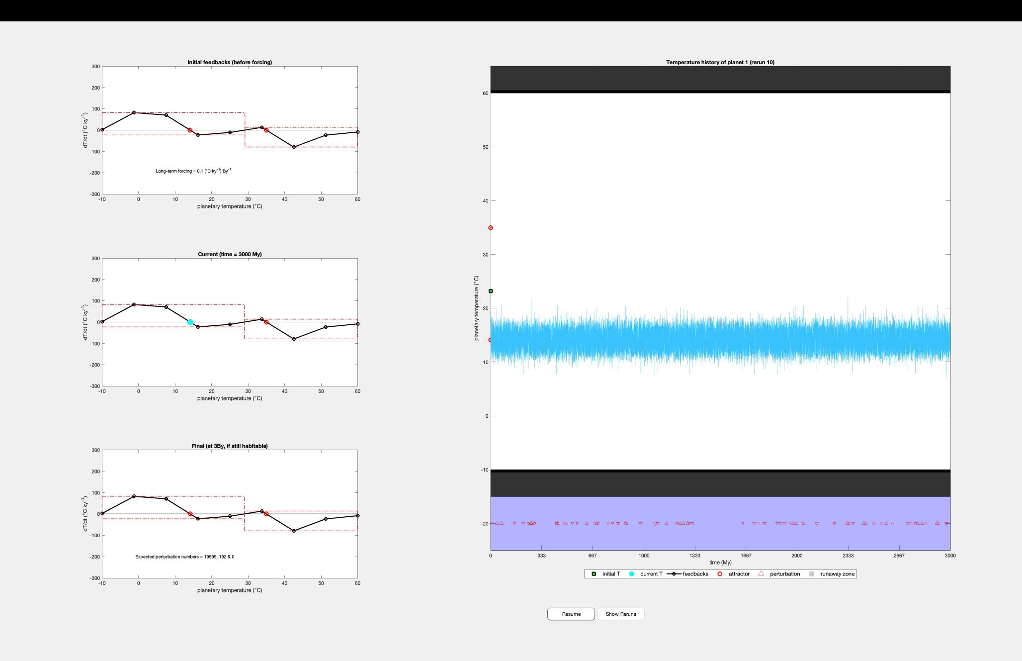
(a) Graph for final rerun of optimal planet. The graphs on the left represent initial conditions of the planet before forcing (top), current temperature (blue dot) vs change in temperature over time and after forcing (middle), and the final conditions (bottom graph)

(b) 4 of the 10 reruns for the optimal planet are shown. The graphs each show the planetary temperature as a function of time in Millions of years. Perturbations are represented by triangles along the x-axis, varying in size depending on the type of perturbation. The green square represents the initial temperature, and the red circles represent the nodes. Grey represents runaway feedbacks (i.e. temperature will irreversibly increase or decrease).
The optimal planet remained habitable for 3 billion years in all 10 reruns. 4 of them are shown in 1b. The long-term forcing that was calculated for the optimal planet was 0.1 ◦C ky 1 per billion years. The value for long-term forcing is consistent with the expected values, as are the feedbacks. In order to maximize habitability, the temperature should remain as constant as possible.
Figure 1: Long-term habitability for Teegarden’s Star b
The overall flat trend seen in Figure 1b is also expected. Since temperature must attract towards a node, the temperature shifts almost instantly to the nearest node and stays constant. Due to the low frequency of higher perturbations, the temperature also cannot shift between nodes.
Teegarden’s Star b
While all 70 planets were tested, only 27 had at least 2 successful runs of long-term habitability. They generally grouped around ESIs of 0.80, 0.85, and 0.94. The planet with the highest successful reruns was Teegarden’s Star b. It has an Earth Similarity Index of 0.97, a radius of ∼ 1.05 Earth radii, 116% of Earth’s mass, and an average stellar flux of 1.08 SE.
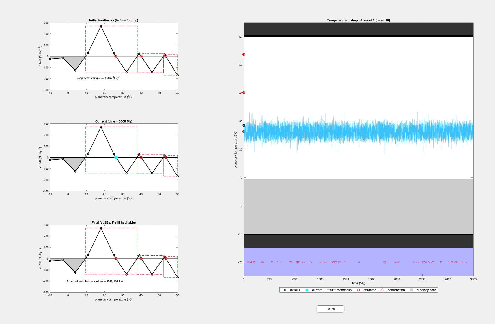
(a) Graph for final rerun of Teegarden’s Star b. The graphs on the left represent initial conditions of the planet before and after forcing (top 2), and the final conditions (bottom graph)

(b) graph of first four reruns of Teegarden’s Star b. The symbols represent the same things as in1b
Figure 2: Long-term habitability for Teegarden’s Star b
Teegarden’s Star b had the highest successful reruns of all the planets, remaining habitable for 7 of 10 reruns. It failed the first, second, and eighth reruns. The long-term forcing was 0.8 ◦C ly 1 per billion years, which explains the constant trend after reaching the node. The behavior that Teegarden’s Star b exhibited is most like the optimal planet (See Figure 1a.
The temperature trend for tea portrays an almost ideal. The initial feedbacks before forcing (Figure 2a top left graph) shows a closer relationship to the trend for the optimal planet than other planets tested. This is also supported by real world data; given that Teegarden’s Star b’s ESI score is 0.97. Additionally, in Figure 2b we see a similar initial shift towards nodes, followed by no significant
change in temperature over time. However, it should be noted that there are significantly more medium-sized perturbations, which can lead to a shift between nodes (see Figure 2b rerun 4).
TRAPPIST-1 e
The planet with the highest long-term habitability rate among the 0.85 ESI grouping was TRAPPIST-1 e. TRAPPIST-1 is an M-type star. Meaning it has relatively low luminosity and a higher variability in solar wind, which leads to a more unstable environment for the planet. TRAPPIST-1 e is an earth sized planet (0.92 RE), with mass of 0.69 Earth masses. Its stellar flux is 0.65 as large as Earth’s.

(a) Graph for final rerun of TRAPPIST-1 e, including initial conditions before and after forcing.

(b) graph of first four reruns of TRAPPIST-1 e.
Figure 3: Long-term habitability for Teegarden’s Star b
The simulation of TRAPPIST-1 e had 4 successful reruns, although the 6th rerun, which attracted to a similar node as rerun 4 came within 0.3 billion years of the cutoff. The high long-term forcing calculated (54.8◦C ly 1) per billion years) was significantly higher than that other planets, and there was a higher frequency of medium-sized perturbations for each rerun.
Since TRAPPIST-1 b is a M-type star, it is subject to higher variability in stellar flux, as well as a habitable zone very close to the star. This results in a high amount of energy being received by the planet. The planet’s small size works to somewhat counteract the star’s effect, but it’s not enough. The high fluctuations in solar wind
eventually degrade the planet’s atmosphere, which leads to lower temperatures, because there is significantly less greenhouse effect (Cohen et al., 2024)((Van Looveren et al., 2024). The high long-term forcing calculated (54.8◦C ly 1 per billion years) was due to this high degradation of the planet’s atmosphere).
Furthermore, because of the star’s variability, there is a higher frequency of medium to large-sized perturbations. This significantly impacts the planet’s long-term habitability because there is a greater chance of runaway feedback (denoted by grey areas in the graphs), which would cause the temperature to fall or rise (in this case, fall) irreversibly until the planet is no longer habitable.
This runaway feedback also explains the 2nd and 3rd reruns in Figure 3b. The planet became uninhabitable since the initial temperature (denoted by the green square) was within this runaway zone.
Kepler-1410 b
The planet with the most successful runs among those in the 0.80 ESI range was Kepler-1410 b. It is a K-type star. Meaning it is significantly hotter and more luminous than the sun. However, their size is also about .70 times the radius of the sun, so the stellar flux is relatively the same as for Earth (1.07 SE). Kepler-1410 b has an ESI of 0.80, radius of 1.78 RE, and mass of ∼ 3.82 ME. It is categorized as a super earth.

(a) Graph for final rerun of Kepler-1410 b, including initial conditions before and after forcing.

(b) graph of first four reruns of Kepler-1410 b.
Figure 4: Long-term habitability for Teegarden’s Star b
Figure 4 shows a greater fluctuation in temperature compared to the other 2 planets. The forcing graphs reveal a high number of fluctuations in temperature over time, with large magnitudes. It should be noted that despite a net negative long-term forcing of -1.8 (◦C ly 1) By 1, the temperature has a positive increase after each node except the last. As a result, the temperature vs. time graph of the planet tends to increase over time until it reaches the last node. In some cases, it skips nodes altogether (see Figure 4b rerun 4). In the 10 reruns of Kepler-1410 b, only 3 survived. Kepler1410 b is the most interesting example among the planets shown because it has the most variable temperature of all.
The planet is orbiting a K-type star, which has a very high temperature (and flux). Its orbital distance is also very close to the star, so (like TRAPPIST-1 b), it loses part of its atmosphere. However, because of its large surface area, it’s not prone to as much cooling as TRAPPIST-1 b. This means that its temperature will actually increase as it loses its atmosphere, resulting in an upward trend in temperature. The model supports this idea (see Figure 4b). In the first rerun, we see the temperature attract from one node to another due to a medium perturbation, and then almost immediately after, it increases to 50 ◦C. Additionally, the increased sensitivity to feedbacks, as well as the increased frequency of higher level feedbacks results in the low habitability of the planet. Since the planet tends to attract to higher nodes rapidly, and once it’s reached, the high frequency of medium-high level feedbacks almost ensures that the planet will become too hot to support the evolution of intelligent life.
Conclusion and Future Work
The implication from these results is that direct observations of other planets can be combined with simplistic, probability-based habitability models to accurately track habitability over time frames long enough for intelligent life to develop. Currently, the main limitation to this finding is that there aren’t enough observations on exoplanets. This limits the accuracy of the model for planets with unknown properties. However, as telescopes become more and more powerful, these limits are expected to improve (especially with the JWST). Since this approach is based on probability, future studies should use higher sample sizes and run each one more times to attain more accurate results.
Acknowledgements
This research has made use of the NASA Exoplanet Archive, which is operated by the California Institute of Technology, under contract with the National Aeronautics and Space Administration under the Exoplanet Exploration Program.
References
Tyrrell, T. (2020). Chance played a role in determining whether Earth stayed habitable. Communications Earth & Environment, 1(1). https://doi.org/10.1038/s4324702000057-8
Schlichting, H. E. (2018). Formation of Super-Earths. Handbook of Exoplanets, 1–20. https://doi.org/10.1007/978-3-31930648-3141 − 1
Cohen,O.,Glocer,A.,Garraffo,C.,Alvarado Gomez,J.D.,Drake,J.J., Monsch,K.,´&FauthPuigdomeorbitexoplanetsbytheirrapido rbitalmotionthroughanextremespaceenvironment.TheAstrop hysicalJournal, doi.org/10.3847/1538 − 4357/ad206a
Van Looveren, G., Gu¨del, M., Boro Saikia, S., & Kislyakova, K. (2024). Airy worlds or barren rocks? On the survivability of secondary atmospheres around the TRAPPIST-1 planets. Astronomy & Astrophysics, 683. https://doi.org/10.1051/0004-6361/202348079
NASA’s Exoplanet Archive https://doi.org/10.26133/NEA12
PHL at UPR Arecibo (YEAR, MONTH DAY). The Habitable Worlds Catalog (HWC). http://phl.upr.edu/hwc
Jagadeesh, M. K., Valluri, S. R., Kari, V., Kubska, K., & Kaczmarek, L. (2020). Indexing exoplanets with physical conditions potentially suitable for rock-dependent extremophiles. Life (Basel, Switzerland), 10(2), 10. doi: 10.3390/life10020010. 10.3390/life10020010
Jingxuan Yang, Patrick G J Irwin, Joanna K Barstow. (2023). , Testing 2D temperature models in bayesian retrievals of atmospheric properties from hot jupiter phase curves. Monthly Notices of the Royal Astronomical Society Pages, 525(4), 5146–5167. https://doi.org/10.1093/mnras/stad2555
Kasting, J. F., Whitmire, D. P., & Reynolds, R. T. (1993). Habitable zones around main sequence stars. Icarus, 101(1), 108–128. 10.1006/icar.1993.1010
Thompson, S. E., Coughlin, J. L., Hoffman, K., Mullally, F., Christiansen, J. L., Burke, C. J., Bryson, S., Batalha, N., Haas, M. R., Catanzarite, J., Rowe, J. F., Barentsen, G., Caldwell, D. A., Clarke, B. D., Jenkins, J. M., Li, J., Latham, D. W., Lissauer, J. J., Mathur, S., . . . Borucki, W. J. (2018). PLANETARY CANDIDATES OBSERVED BY kepler. VIII. A FULLY AUTOMATED CATALOG WITH MEASURED COMPLETENESS AND RELIABILITY BASED ON DATA RELEASE 25. The Astrophysical Journal.Supplement Series, 235(2), 38. doi: 10.3847/1538–4365/aab4f9. Epub 2018 Apr 9. 10.3847/1538-4365/aab4f9
Yang, J., Alday, J., & Irwin, P. (2024). Nemesispy [computer software]. Journal of Open Source Software, vol. 9, issue 101, id. 6874:10.21105/joss.06874