Egor Lazarevich
Senior Thesis | 2025

ON
SOME ASPECTS OF COMPUTER PROGRAMMING OF BUSINESS SIMULATION: AN EXAMPLE OF DEVELOPING A “NATIONAL ECONOMY DEVELOPMENT” SIMULATION
ABSTRACT:
Scientific research on the factors and conditions ensuring social and economic development and sustainable growth has long been the focus of many economic researchers. It has become increasingly clear to them that real-life socio-economic systems are prohibitively challenging to formalize mathematically in all detail. Hence, an accurate quantitative description remains resistant to our attempts. One way of coping with this problem and yet to get meaningful, if somewhat generalized and broad, predictions and forecasts regarding the reality of development is to restrict the analysis to a limited set of macroeconomic factors as fundamentals driving the system’s behavior. A business simulation was developed based on the premises of this framework in the form of an interactive computer program.
INTRODUCTION:
Human society is a complex, non-equilibrium system constantly evolving and changing. One of the essential aspects of the study of socio-economic processes in society is macroeconomic indicators. This simulation (sometimes referred to as a model) examines the behavior of a country’s economy as one large corporation. This model can predict the behavior of a country’s macroeconomic indicators depending on the use of new technologies, new equipment, tax levels, wages, etc. The basic assumptions behind the adopted model are as follows:
● A national economy (a country) performs as a single diversified financial holding company comprising several otherwise autonomous operational divisions (called towns), each consisting of production units.
● The source of capital investment and financing is external relative to the economy.
● Income per worker serves only two functions: the rate of employment/unemployment and the population dynamics over time.
Based on this model, the program helps identify possible scenarios of further change in the factors of interest and estimate the resulting development in demographic and economic situations for each scenario.
The work pursued three main objectives:
● To develop a computer-based business simulation to realize the model described above.
● To identify possible results using the program, depending on the values of variables such as technology, plant, wages, and taxes.
● To estimate the values of the model's key parameters from the data available in several countries; to conduct a comparative analysis of changes in national economic and demographic indicators.
MATHEMATICAL MODEL USED:
The country is modeled as a set of independent cities, each serving as an abstract shell for enterprises. Each enterprise can have numerous production facilities and a certain amount of means of production, which is a necessary condition for producing any products, of course if there are sufficient technologies for the given production process. It’s also worth noting that each enterprise has employees, the number of which depends on a particular set of factors and can change over time.
In addition, it’s worth noting that the current model does not consider marketing, logistics, and other components of the production economy. However, within the assumptions, enterprises and their employees are taxed in favor of the state according to a simplified scheme and a fixed percentage rate.
Let’s consider each economic object in more detail:
State:
In this model, the state's role is limited to setting interest rates and collecting taxes from enterprises and their employees. The central bank is not allocated as a separate regulatory body but is combined with the state itself for abstraction. Also, within the framework of this model, the regulatory and administrative levers of the state, internal costs for maintaining budget items that do not generate direct income, inflationary and deflationary processes are not taken into account, and foreign trade relations with other states, as a class, are entirely ignored.
Taxes:
Taxes from the population are deducted in favor of the city budget in the form of a fixed percentage of wages paid to employees at the enterprises where they work: ! = # ⋅ !%&'#
where s is the wage rate, taxes is the tax rate, and t is the amount collected.
The tax rate on the population is the same for everyone and is determined by the state, which is the regulatory body within the model.
Taxes from enterprises, in turn, are also deducted in favor of the city budget and are determined as a percentage of the enterprise’s income according to a scheme similar to that described above.
Enterprise:
Under this model, opening a new enterprise requires a loan from the Central Bank, an integral part of the state. The various types of loans are described below.
The Cobb-Douglas production function determines the production of each enterprise: ( = ) ⋅ * ! ⋅ +" !
where K is engaged capital, L is engaged labor, α and C are some constants, and Y is output.
As classics in economic theory show (1, 2, 3), the CobbDouglas production function depends mostly on capital, both materialistic (equipment, investments, etc.) and human resources (not necessarily salary dependencies, but the amount of labor and their motivation and qualification). In the original 1928 formula , = - ⋅ +$ ⋅ ) " $ , the authors tried to evaluate the coefficient k. In the USA, in 1904, this value was assessed to be 0.65; in 1919, it was 0.76; in Australia, in 1956, it was 0.615; in 1968, it was 0.536. This clearly shows the non-constant and nonmonotonic nature of this coefficient. The Cobb-Douglas function is still the most ubiquitous tool in theoretical and empirical analysis of growth and productivity, widely used to represent the relationship of output to inputs (4).
The following formula determines the engaged capital K: * = . ⋅ /'01%/%!234
Where k is the means of production, degradation is the degradation coefficient.
/'01%/%!234 = / ⋅ !
where d is the equipment degradation coefficient, which is some constant, and t is the time elapsed since the equipment was updated.
When the degradation coefficient becomes less than the critical degradation threshold, set as a constant critical in the model, the enterprise is forced to update its production facilities. When updating production facilities, the time t is reset to zero.
Enterprise profit is determined as follows:
634'7 = (#38/ ⋅ (& &% )
Where Money is enterprise profit, Ysold is the number of product units sold, x is the product's unit price, and &% is the unit
cost of raw materials, equal to a constant. A separate case is considered when not all products are sold. In this case, within the framework of this model, the remaining products are sent to an unlimited-size warehouse, where a certain percentage of their cost is charged for storage. Although the model does not take into account factors such as transportation costs, logistics costs, product shelf life, commodity loans, and other aspects of working with retailers, it is assumed within the model that a specific part of the products is simply “lost” in the warehouse over time. It is also assumed that when stored in a warehouse, the enterprise loses money proportional to the amount of stored goods, their cost, and a specific coefficient of financial loss.
The model introduces the assumption that all manufactured products are sold abroad, i.e., the source of money is external.
Export function:
Sales abroad are determined by the formula: < = =31'204>3'== ⋅ & &
Where n is the number of product units sold, foreigncoeff and β are some constants, and x is the price set by the factory.
Loans:
Within this model, a loan for production needed from the Central Bank can be of two types:
● Annuity, i.e., paid in equal shares at time intervals during the entire loan period (the principle for calculating an annuity loan will be given in the section devoted to the program description)
● Proportional, i.e., paid in the form of a particular constant amount + interest in each fixed period. The formula for a proportional loan looks like this: #?@ = '(()*+ , + '4/#?@ ⋅ >1'/2!B13> '4/#?@ = %88#?@ %88#?@ ⋅ 4 <
where sum is the amount of the loan paid this month, allsum is the total loan amount, N is the loan term, creditproc is the interest rate, endsum is the amount left to pay, and n is how many months ago the loan was taken. In case of non-payment of the loan, an abstract process of enterprise bankruptcy is launched and all people employed there are transferred to the unemployed status. The legal and economic intricacies of bankruptcy remain outside the scope of this model.
People:
This model operates with two types of people:
● Employed in production, i.e., listed on the balance sheet of their enterprises and receiving wages.
● Unemployed, i.e., receiving a minimum unemployment benefit paid by the state.
Each month, the number of people of both types is multiplied by the following coefficient:
B'3B8'>3'== = 1 + . ⋅ 84( > >% )
where k is the viability coefficient, c is the money received (salary after paying taxes), and c0 is the subsistence minimum at which the population does not change. The hyperbolic growth model can also estimate population doubling times, which are not constant but vary with time, mirroring real-world data (5). This model can also answer interesting questions like how many people have lived on Earth since the year 0 (about 54 billion) or since the dawn of history (about 107 billion, close to current estimates).
COMPUTER PROGRAM:
A computer simulation program had been developed for the mathematical model described. The program uses an input file in text format, and input data closely corresponds to a hierarchical data structure.
The program outline:
The CCountry class is the main class, containing CTown, CBank, CGovernment, CMoney, and other subobjects.
After data reading and displaying the primary cycle is executed. It calls method nextMonth for the country object. The same method then calls for all town subobjects and factories and workers.
CCreditAccount class describes a credit model. There are two kinds of credits: annuitant and proportional. CTownclass describes the town as a set of subobjects: factories list, unemployed workers, templates for new factories, tax collectors, and trends for money and population.
CTown class has methods nextMonth that calls a similar method for mutable subobjects.
CPeople class describes the properties of workers, such as productivity and relative salary. According to the financial month results, the factory pays all the workers a wage. If the salary exceeds the life minimum, then the population increases. If the factory closes, all its workers will become unemployed. The replication rate defines the level of growth of the population if the salary is greater than the minimum life level.
The CFactory class describes the factory as a set of productivity tools.
The problem of calculating the price of production to get maximum profit requires solving an optimization problem. The solver method is CMoney.getOptimalExportAndStorageCost uses calcExportValueByCostDerivation to compute the derivation of the profit function.
CTool class denotes a model of the production tool. Each tool has a cost and produces CProductionItem. Degrading property is part of the production capacity left after one month. When degradation lowers as low as FundRepairLimit, the tool is not usable anymore and must be replaced by another.
The CProductionItem class describes a unit of production. It has a base cost and a laboriousness.
Class CTechnology describes production technology as a tool for production. The Cobb-Douglas law determines the number of outputs and depends on the funds.
Class CExport determines the rules under which it calculates the amount of the product that can be exported, i.e., in this open model, is sold. It has a primary method willBeExported, which determines the required number of units.
The CStorage class describes the storage model for product items. Assume that the warehouse is unlimited, but the storage of products leads to the loss of production (parameter MonthlyProductionLoss) and overheads for storage (Taxes), that is, the loss of both products and cash.

The program's object model structure is shown in Fig. 1.
Figure 1: Structure of the Object Model
SOME RESULTS:
The experiments produced model input data of two cities with the same parameters, except for one variation.
Determining the influence of the parameter productivity (the parameter in the Productivity section PeoplePattern):

Figure 2: Determining of the Influence of the Parameter Productivity
In the top row of graphs here and other cases, the result shows the base, lower, which is the result of a change of the parameter. In this case, the parameter Productivity=0.30 has replaced Productivity=0.15. The decrease in the population is wellmarked in the base case. It is also noticeable that the systematic reduction in the enterprise funds in the base case changed to a sufficiently stable state.
Determining the Influence of the Coefficient of Reserve Funds:
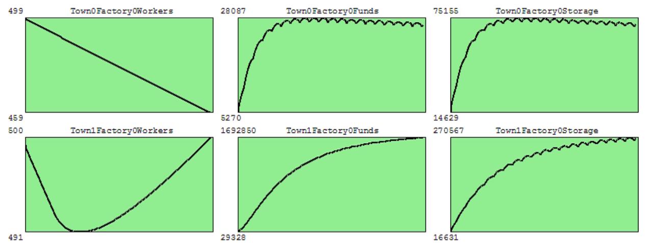
Figure 3: Determining the Influence of the Coefficient of Reserve Funds
Coefficient FundsReserve determines which part of the enterprise's current assets must be reserved for the next month and does not give the fund the salary changed from 0.25 to 0.85.
The result is paradoxical at first glance, with a decrease in wages and population growth from a specific period. However, this can be explained by the fact that a large flow of funds to the technology ultimately leads to increased production and, ultimately, to an increase in wages and population size.
Determining the influence factor limits the Hardware Update (FundsRepairLimit). This ratio changed from 0.8 to 0.5:
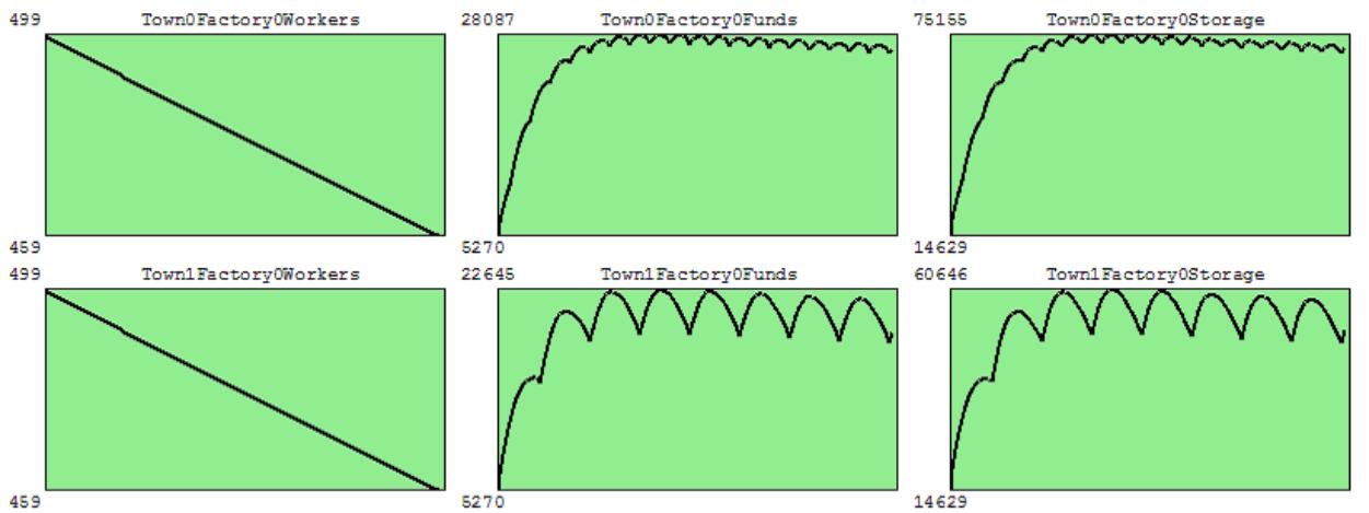
Figure 4: Determining the Influence Factor Limits the Hardware Update
Again, the paradoxical result at first sight was that the number of workers remained the same, but the enterprise funds for a few equipment replacements took up a smaller maximum. This is because the equipment works quite a lot in the second case of low efficiency.
Determination of the influence of loss of deposit (MonthlyProductionLoss):

Figure 5: Determination of the Influence of Loss of Deposit
With increased productivity, ratios changed to 0.35, with 0.08 monthly production load to 0.06. The result was expected:
improving the efficiency of the enterprise leads to an increase in all parameters.
COMPARING THE RESULTS SECTION TO REALWORLD EXAMPLES:
Influence of Productivity on Economic Growth:
The experimental results show that an increase in the productivity parameter (from 0.15 to 0.30) results in a marked decrease in population in the base case. At the same time, the enterprise funds begin to stabilize after an initial reduction. These results align with real-world economic instances in which shifts in productivity impact labor markets and financial stability.
One example is Japan, where high productivity and automatic manufacturing equipment have contributed to economic growth and a shrinking workforce because of a declining birth rate and reduced demand for human labor. Similarly, industrial automation in the U.S. led to job displacement in specific areas, decreasing the labor requirement in that area and necessitating labor transition to new industries. However, developing nations with increased productivity tend to experience population growth as higher wages lead to improved living conditions, reduced mortality rates, and increased migration inflows, which contradicts this trend, and it would be interesting to try to include this distinction between already developed economies and developing economies into the model.
Additionally, in highly automated industries, like semiconductor manufacturing, increased productivity lessens the need for unskilled labor while creating a higher demand for specialized professionals. My model assumes that there is only one type of job; however, trying to model education levels and job tiers and seeing how productivity increases change the demographics would be interesting. This shift from unskilled to skilled labor highlights the need for retraining and education policies to help the
workforce adapt to changing economic conditions. Countries not implementing retraining policies may face long-term employment and productivity challenges despite, in theory, having a highly productive industrial base.
Influence of Reserve Fund Coefficients on Wages and Population Growth:
The experiment found that increasing the coefficient of reserve funds (from 0.25 to 0.85) paradoxically led to decreased wages but increased population growth over time. The explanation is that higher savings toward technology investment boost production and wages.
This same trend can be observed in emerging economies where the emphasis is placed on reinvestment into technology and infrastructure as opposed to wages. For example, South Korea’s post-war economy invested heavily in automation while keeping wages tight. Over time, this increase in productivity resulted in economic growth, higher wages, and an increased standard of living.
Another real-world example is China’s economic policy where corporate spending and government-driven reinvestments in infrastructure and technology initially kept wages low. However, the wages rose as the industries became more productive leading to population and economic growth. The model supports the notion that reinvestment and expansion lead to substantial benefits.
Additionally capital-intensive sectors like aerospace and energy keep critical reserve funds to ensure stability during market downturns. This sets them up nicely to grow well once the market restabilizes. Another notable example is Tesla where reinvestment in research and development initially limited profitability and kept wages low but over time technological advancements allowed for massive scalability and increased wages.
Financial reserves also play a crucial role in economic resilience during crises. The COVID-19 pandemic showed how
companies and nations with substantial reserve funds were better equipped to sustain economic activity and recover more quickly than those with minimal reserves. This observation reinforces the finding that long-term financial stability often requires short-term sacrifices.
Influence of Hardware Update Limits on Enterprise Funds:
In the experiment, reducing the FundsRepairLimit parameter from 0.8 to 0.5 as expected led to a situation where enterprise funds for equipment replacement decreased, however the number of employees remained constant. The explanation is that the equipment, despite its lower efficiency, continued to operate and therefore the number of workers needed to remain constant to operate the equipment which is what was expected. This same trend can be observed in industries that delay capital investment into new machinery to maintain liquidity. An example is many companies during the 2008 financial crisis where many companies delayed capital investment because of economic instability. Firms like manufacturing or airlines continue to operate old equipment. This decision resulted in lower efficiency but stable employment levels.
On the other hand, industries such as technology and energy which require constant hardware upgrades did not follow this trend. Companies that delayed technological reinvestment eventually fell behind a result that the model supports since delaying reinvestment stabilizes short-term financials but leads to long-term inefficiencies.
Industries that rely on advanced robotics and AI-driven automation must invest in both hardware lifecycles and innovation. Firms that do not maintain this rapid pace of modernizing their infrastructure risk falling behind their competitors who leverage modernized efficient systems. This is especially relevant in the semiconductor industry where firms like Intel and TSMC
continuously reinvest in next-generation equipment to maintain a competitive edge.
A broader implication is that governments and businesses must implement policies encouraging capital reinvestment to delay the adverse effects of lagging infrastructure. Incentives such as tax credits for technological upgrades or subsidies for research and development can make sure economic growth remains steady this leads to increased capital which can be reinvested again to start a cycle of constantly improving productivity.
Influence of Monthly Production Loss on Economic Efficiency:
The model predicts that reducing monthly production loss (from 0.08 to 0.06) this improved productivity increase all the parameters including enterprise funds, wages, and population growth. This is to be expected since in the real world efficiency drives improvements in quality of life and economic expansion.
One great example of this trend is the implementation of digital technologies in logistics and supply chains. Companies like Amazon have used predictive analytics and automation to reduce inefficiency, leading to increased productivity and profitability. My model supports this showing that a decrease in inefficiencies raises all the economic parameters of the company in multiple dimensions.
Another example is the agriculture sector where advanced precision farming techniques including satellite-based monitoring and automated irrigation systems, have decreased production loss and increased yield. The model supports this, reducing any amount of inefficiency is a really substantial step towards economic stability and growth.
In the same vein industries where the product is perishable such as food processing have adopted cold-chain logistics to minimize any losses. Companies reduce inefficiencies by investing in efficient transportation and storage systems, leading to a constant production output and revenue stream.
One important takeaway is that reducing inefficiencies should not just be a company concern but a national priority. Countries with bloated bureaucracies and outdated infrastructure tend so see their economic growth stall. In contrast, nations that nations that invest heavily into keeping infrastructure modern see sustained economic expansion reinforcing the idea that reducing inefficiency is essential on both a micro and macroeconomic level.
CONCLUSION:
This paper describes the mathematical model of economic processes in a single country. The country is considered a diversified financial holding company with several divisions that make production units per turn. Each production unit has a certain amount of plant, machinery, and soft capital in the form of technology used. The model treats the staff employed by a production unit as an asset on its balance sheet. The workforce's size depends on multiple factors and can vary over time. The framework does not account for some real-life business activities, such as marketing and logistics. A set of scenarios with variations of parameters was performed, and the mathematical model was found to be consistent. In addition to testing the model’s internal consistency, the model was also compared against real-world examples, and the outputs of the model given a particular set of parameters were tested against real-world outcomes. This comparison showed that the general trends illuminated by the model manifest, albeit with some exceptions in the real world. For instance, automation led to a decrease in labor capacity and a stabilization of enterprise funding which mirrors economies such as Japan, where the increase in productivity led to a shrinking population and a decreasing workforce; another example is the US, where an increase in productivity in specific sectors drove people to find different careers. However, in developing economies, this trend is reversed; the increase in wages due to productivity increases raises levels of birth rates, quality of life, and
immigration. An interesting study would be to model the difference between an already established economy becoming more efficient and a developing economy gaining efficiency. Additionally, considering factors like education levels and job tiers could reveal new trends. Also, the model's simulation of lowered hardware update limits reflects how companies react to economic downturns like the 2008 financial crisis. Industries that delayed technological investments lost momentum, while the sectors that continued innovating only pulled further ahead. As predicted by the model, the reduction in monthly production loss mirrors efficiency improvements in industries like automotive manufacturing, digital logistics, and agriculture, where innovation in production processes leads to increased profitability and stability. Potential applications of this model include educational tools for economics students to visualize different macroeconomic principles, policy simulation for government officials to test potential economic interventions, planning tools for large corporations to model market dynamics, and research platforms for economists to study complicated financial systems. Further development could include adapting the model to specific industry sectors or incorporating more detailed international trade dynamics.
REFERENCES:
[1] P. H. Douglas. “The Cobb-Douglas production function once again: its history, its testing, and some new empirical values,” Journal of Political Economy, vol. 84, no. 5, pp. 903–915, 1976, The University of Chicago Press.
[2] J. M. Clark, “Inductive evidence on marginal productivity,” The American Economic Review, vol. 18, no. 3, pp. 450–467, 1928, JSTOR.
[3] J. Biddle, “Retrospectives: The introduction of the Cobb–Douglas regression,” Journal of Economic Perspectives, vol. 26, no. 2, pp. 223–236, 2012, American Economic Association.
[4] J. Chisasa, D. Makina, et al., “Bank credit and agricultural output in South Africa: A Cobb-Douglas empirical analysis,” International Business & Economics Research Journal (IBER), vol. 12, no. 4, pp. 387–398, 2013.
[5] D. Hathout, “Modeling population growth: exponential and hyperbolic modeling,” 2013, Scientific Research Publishing.
[6] Banks, J., J. S. Carson, B. L. Nelson, and D. M. Nicol. 2000. Discrete-event system simulation. 3d ed. Upper Saddle River, New Jersey: Prentice-Hall, Inc
[7] J. E. Biddle, “Statistical economics, 1900–1950,” History of Political Economy, vol. 31, no. 4, pp. 607–651, 1999, Duke University Press.
[8] C. W. Cobb, “Production in Massachusetts manufacturing, 1890–1928,” Journal of Political Economy, vol. 38, no. 6, pp. 705–707, 1930, The University of Chicago Press.
[9] C. W. Cobb and P. H. Douglas, “A theory of production,” American Economic Review, Papers and Proceedings of the Fortieth Annual Meeting of the American Economic Association, vol. 18, no. 1, Supplement, pp. 139–165, 1928, American Economic Association.
[10] P. H. Douglas, “The problem of labor turnover,” American Economic Review, vol. 8, no. 2, pp. 306–316, 1918, American Economic Association.
[11] P. H. Douglas, “Is the new immigration more unskilled than the old?” Publications of the American Statistical Association, vol. 16, no. 126, pp. 393–403, 1919, Taylor & Francis.
[12] P. H. Douglas, Real Wages in the United States, 1890–1926, New York: Houghton Mifflin, 1930.
[13] P. H. Douglas, The Theory of Wages, New York: MacMillan, 1934.
[14] P. H. Douglas, “Are there laws of production?” American Economic Review, vol. 38, no. 1, pp. i–ii, 1–41, 1948, American Economic Association.
[15] P. H. Douglas, “The Cobb–Douglas production function once again: Its history, its testing, and some new empirical values,” Journal of Political Economy, vol. 84, no. 5, pp. 903–915, 1976, The University of Chicago Press.
[16] D. Durand, “Some thoughts on marginal productivity, with special reference to Professor Douglas’ analysis,” Journal of Political Economy, vol. 45, no. 6, pp. 740–758, 1937, The University of Chicago Press.
[17] H. Mendershausen, “On the significance of Professor Douglas’ production function,” Econometrica, vol. 6, no. 2, pp. 143–153, 1938, Econometric Society.
[18] M. W. Reder, “Chicago economics: Permanence and change,” Journal of Economic Literature, vol. 20, no. 1, pp. 1–38, 1982, American Economic Association.
[19] P. A. Samuelson, “Paul Douglas’s measurement of production functions and marginal productivities,” Journal of Political Economy, vol. 87, no. 5, Part 1, pp. 923–939, 1979, The University of Chicago Press.
[20] H. Schultz, “Marginal productivity and the general pricing process,” Journal of Political Economy, vol. 37, no. 5, pp. 505–551, 1929, The University of Chicago Press.
[21] A. Shaikh, “Laws of production and laws of algebra: The humbug production function,” Review of Economics and Statistics, vol. 56, no. 1, pp. 115–120, 1974, MIT Press.
[22] S. Slichter, “Economic and social aspects of increased productive efficiency Discussion,” American Economic Review, Papers and Proceedings of the Fortieth Annual Meeting of the American Economic Association, vol. 18, no. 1, Supplement, pp. 166–170, 1928, American Economic Association.
[23] R. Solow, “Technical change and the aggregate production function,” Review of Economics and Statistics, vol. 39, no. 3, pp. 312–320, 1957, MIT Press.
[24] R. Solow, “Law of production and laws of algebra: The humbug production function: A comment,” Review of Economics and Statistics, vol. 56, no. 1, p. 121, 1974, MIT Press.
[25] G. J. Stigler, Production and Distribution Theories: The Formative Period, New York: MacMillan, 1941.