
Validation of Machine Learning Algorithms for Identifying Sharp-Wave Ripples in Epileptic Conditions
Senior Thesis | 2025

Validation of Machine Learning Algorithms for Identifying Sharp-Wave Ripples in Epileptic Conditions
Ajay Wadhwani
Abstract
Mesial temporal lobe epilepsy is the most common drug-resistant epilepsy syndrome. Many patients with this disorder suffer from memory dysfunction as hippocampal seizures can impact memory. Surgical resections, although they can cure seizures, often worsen memory.1 Sharp wave ripples are the most synchronous patterns in the mammalian brain, detected in the hippocampal CA1 layer. They are transient fast oscillatory events (100-250 Hz) and biomarkers for memory consolidation.2 However, spike ripples, a pathological biomarker for seizures in an epileptic hippocampus, share similar properties with sharp wave ripples. These events are not well understood and cannot be reliably classified using current detectors.3 Machine learning (ML) approaches provide new opportunities to classify subtle differences in rhythms. Recently several ML approaches were proposed and found to be successful in detecting SWR in rodents and non-human primates.4 For this project, the RipplAI toolbox was used, which was shown to be successful in detecting SWRs in mice and macaque hippocampus. The goal of this project was to evaluate the accuracy of ML approaches used in RipplAI to detect SWR in human recordings and in the setting of epileptic activity. While these models were able to detect some SWRs in humans, they were much less effective and would require further retraining to be useful.
1 (Mathon et al., 2017)
2 (Joo & Frank, 2018)
3 (Kramer et al., 2019)
4 (Navas-Olive et al., 2024)
Introduction
Mesial Temporal Lobe Epilepsy (MTLE)
Epilepsy, a neurological disease-causing recurring seizures, affects over 50 million people worldwide. While seizures can be curbed through medications in most forms of epilepsy, some kinds of this disease are known as drug refractory, meaning they do not respond well to current medications. Mesial temporal lobe epilepsy (MTLE) associated with hippocampal sclerosis is the most common drug refractory form of epilepsy. Because the hippocampus is a part of the brain important for memory function, hippocampal seizures caused by MTLE cause memory impairment issues to those who suffer from it. Treatments of MTLE include surgical resections of the hippocampus, in which the epileptic portion of the hippocampus is removed, such as anterior temporal lobectomy (ATL) or selective amygdalohippocampectomy (SAH). While surgical resections have been shown to reduce seizure frequency in 62-83% of patients, they have also been shown to reduce memory function after the operation in close to half of patients, causing worsened cognitive and/or verbal memory. However, there are also other non-resective surgical options such as implanted devices that can deliver electrical signals to the brain to help treat seizures. Because of this, it is important to be able to identify healthy hippocampi to better know how to treat MTLE patients.5
Sharp Wave Ripples (SWR)
The hippocampus is also home to sharp wave ripples (SWRs). SWRs are the most synchronized neural patterns in the mammalian
5 (Mathon et al., 2017)
brain, causing a large number of neurons, a neuronal ensemble, to fire in a highly coordinated manner. These events are made up of short, fast oscillatory electrical signals (100-250 Hz) superimposed on slower sharp waves, and they last for around 50 ms. SWRs have been primarily observed in the CA1 layer of the hippocampus during periods of rest, quiet wakefulness, and slow wave sleep. They can be observed through electrophysiological methods such as Local Field Potentials (LFP) and Electroencephalography (EEG). LFPs are recorded using microelectrodes implanted in the brain and are commonly used in animal research for more precise recordings. EEGs, on the other hand, are recorded non-invasively through electrodes placed on the scalp, and are more commonly used in human research.6 Sharp wave ripples have been identified as key components of memory consolidation, a process through which memories are strengthened and transformed into a more long-term form. SWRs work by “replaying” neural activity patterns from periods of learning, as displayed in Figure 1. This process of replay helps the hippocampus solidify memories and allows it to transfer them to the cortex for long term storage. The relationship of SWRs to memory consolidation has been studied in various mammals, including mice, rabbits, monkeys, and humans.
7
6 (Lopes da Silva, 2013)
7 (Joo & Frank, 2018)

Figure 1: Observation of memory consolidation through SWR events. During the period of rest (right), the rat experiences SWR events similar to patterns experienced during active learning (left).

Figure 2: Anatomy of the hippocampus, highlighting the CA1, CA3, and stratum pyramidale regions where SWRs take place.
SWRs found in the CA1 region generally follow a similar pattern. They include a high frequency ripple in the stratum pyramidale layer of the hippocampus, where numerous pyramidal neurons are located, and a sharp wave deflection in the stratum radiatum, caused by strong excitatory signals from the CA3 region. However, SWRs are not always identical, and they can vary a lot depending on the neural circuits being reactivated. Different memory traces or experiences being replayed will cause different circuits to activate. Most current methods for SWR detection are spectral, meaning that they only analyze the frequency of the data. However, these methods are not optimal, as they lack precise timing and can be affected by overlapping frequencies. Because of this, new methods, such as machine learning, are crucial to be able to detect SWR events using spatial, temporal, and frequency-based analysis. 8
Spike Ripples (SR)
Despite receiving the maximum medication, for around one third of epilepsy patients, seizures cannot be controlled. For these select patients, their seizures come from a localized region in the brain, so they require resective surgery to treat them. In order for these surgeries to happen, it is important to be able to identify the epileptogenic zone–the area of the brain responsible for causing the seizures. There are two main biomarkers that help identify the epileptogenic zone: a spike or interictal discharge,or a ripple or high frequency oscillation. Spikes are specific to epilepsy, but occur too broadly to accurately identify the epileptogenic zone. Ripples on the other hand, are more localized, but they are part of both pathological and physiological processes. Although both signals have been researched thoroughly, neither one is specific
8 (Joo & Frank, 2018)
enough to determine treatment options. Because of this, a new signal has been proposed as a biomarker, a “spike ripple” (SR), the simultaneous occurrence of a spike and a ripple in an epileptic brain. This combined event, which occurs in epilepsy patients, allows for more precision in localizing the epileptogenic zone. Spike ripples share morphological characteristics with the physiological sharp wave ripples, both seen in Figure 3. The overlap in properties between SWRs and SRs make it difficult to reliably differentiate between these events using current detection methods. SRs have been generally unstudied, and it is unknown whether they involve the same neuronal ensembles that generate SWRs. It is important to be able to distinguish between these events and understand the neuronal ensembles behind them.9

9 (Kramer et al., 2019)
Hippocampal Project Goals
The Chu Lab, an epilepsy lab housed in the Department of Neurology in Massachusetts General Hospital, is currently working on a project around Hippocampal Epilepsy and Memory. There are three specific aims of this project. The first aim is to understand the cellular networks behind SWR and SR events. To do this, the researchers use advanced imaging and electrophysiological techniques such as the SomArchon voltage imaging sensor to record data from mice. They then induce hippocampal epilepsy in the mice and try to uncover how SWRs and SRs are generated and how they interact in the hippocampus. The second aim is to develop and validate automated detectors using behavior and LFP to distinguish between SWRs and SRs in rodent and human hippocampal recordings. Using knowledge gained from the first aim and a large dataset of human LFP recordings, they label SWRs and SRs during wakeful and seizure periods. They then use this data to train a convolutional neural network to differentiate between SWRs and SRs using visual features. The overarching goal of the detector is to classify epileptic versus healthy hippocampi, predicting hippocampal function and seizure risks. The final aim is to predict memory outcomes after hippocampal surgeries. By studying MTLE patients, measuring their sleep dependent memory consolidation and relating it to their SWR and SR rates, the lab hopes to find a correlation between SWR and SR rates and pre-operative memory performance. They will then use pre-operative SWR and SR rates as biomarkers to predict postoperative memory performance and minimize cognitive deficits.
RipplAI Overview
Liset M de la Prida’s group, The Laboratory of Neural Circuits, is located in Madrid Spain and focuses on studying the neural circuits of the hippocampus in the healthy and epileptic brain. It is part of
the Cajal Institute, Spain’s largest neuroscience research center. In 2024, the lab published a study to analyze and detect SWRs across species. In the study, they created a toolbox of machine learning (ML) architectures, which were the result of a crowdsourced hackathon to detect SWRs in mice. These models were able to perform well when applied to recordings of the macaque hippocampus and revealed shared properties across species. The lab then shared these models as an open source toolbox, allowing future researchers to advance the study of SWRs.10
Research Goals
The goals of this paper align with Aim 2 of the Chu Lab’s Hippocampal Project, to develop and validate automated detectors of SWRs and SRs. The RipplAI ML models were shown to perform well in the rodent and macaque hippocampus. We attempted to see how well the models could identify SWRs in human recordings and, specifically, in the setting of epileptic activity where distinguishing between SWRs and SRs might improve our understanding of MTLE’s effect on memory.
Methods
Hackathon
In the study, “A machine learning toolbox for the analysis of sharp-wave ripples reveals common waveform features across species,” researchers at the Prida Lab ran a crowdsourced hackathon to develop ML detection methods of SWRs. Participants were specifically selected as people unfamiliar with neuroscience and SWRs. The hackathon was comprised of 36 teams of 2-5 people from a variety of academic and professional backgrounds. Participants were given the background information through online courses on neuroscience, Python, and machine learning in the month before the event. They were also familiarized with Python functions for loading the data, evaluating the performance of the models, and displaying the results in a shared format. Finally, they were given a dataset, consisting of LFP recordings from the CA1 layer of the dorsal hippocampus in awake mice. The data included 8 channels of raw unprocessed LFP data, recorded using high density electrical probes and sampled at a frequency of 30,000 Hz. It also included SWR events, which were manually tagged by an expert to be used as ground truth, and the start and end time of these events were recorded. Ground truth events are manually labeled data to help train a ML model. The dataset was split into a training set and validation set. The training set was recorded from two mice and contained a total of 1794 manually labeled SWR events. The validation set was recorded from another group of two mice and contained 1275 labeled events.
The hackathon took place over one weekend in Madrid in October 2021 using remote methods. It lasted 53 hours over the course of three days. From the 36 teams, 18 models were submitted for
consideration at the end. The most popular ML architecture was extreme gradient boosting (XGBoost), used in four solutions. Other popular architectures included one and two dimensional convolutional neural networks (1D and 2D CNN), deep neural networks (DNN), and recurrent neural networks (RNN; See machine learning section for more details). Out of the 18 solutions, five were not functional and could not be ranked. Five of the best performing solutions were selected for further analysis. These models were XGBoost, 1D and 2D CNN, a support vector machine (SVM), and an RNN, specifically the long short-term memory (LSTM) version of the algorithm, which is better suited for temporal data.
The researchers decided to standardize the training process for all the models, as each solution had its own method. The original LFP data was sampled at 30,000 Hz, but to keep the models consistent, they downsampled all the data to 1250 Hz and normalized it using z-scores. The data was randomly divided, 70% into a training set and 30% to validate performance. To optimize the models, the researchers tested a variety of different hyper parameters, such as the number of channels used from the LFP recordings or the size of the analysis window. There were also model specific parameters, such as tree depth for XGBoost, which were tested. Each of the combinations of hyper parameters created a new variation of the models. From these new variations, the 50 best performing models of each type were chosen. The models were validated using F1 score (See section on performance measures below), which showed how close the model’s predictions were to ground truth, and tested on new dataset. They found that the LSTM and 1DCNN models performed the best, with mean F1 scores of about 0.6. Ultimately, the five best models of each architecture were published online in an open source toolbox.
After developing these models which could identify SWRs in mice hippocampi, the researchers wanted to extend the study to nonhuman primates. To do this, they used LFP data from the hippocampus of macaques. First, they applied the models trained on the mouse data to the recordings from the macaque hippocampus. Surprisingly, four out of the five models performed well, reaching a maximum F1 score of around 0.5, which compares to their performance on the mice data (0.6). They then retrained the models based on the macaque dataset and performances improved.11
Machine Learning Methods
There are two kinds of machine learning: supervised and unsupervised. Supervised learning trains a model based on a set of data and labeled data points. This allows the model to learn how to perform a task over time from previous examples where the answer is already given. Some applications of supervised learning are classification, in which the model sorts data into certain categories, and regression, in which the model returns a numerical value as the answer. A benefit of supervised learning is that one can measure the accuracy of models by testing it against the labeled data points. On the other hand, unsupervised learning does not include labeled data points. An unsupervised model is given a set of data and can perform tasks like analysis and clustering to find relationships and patterns in the data that humans could not physically see. Because the study included labeled SWR events and required a classification task, the models were all forms of supervised learning. There were five main models in the toolbox.
11 (Navas-Olive et al., 2024)
XGBoost is a decision tree based algorithm. During training, the algorithm evaluates features of the data, such as LFP values, and splits the data based on threshold values. If the split is correct, it generates new nodes until a maximum tree depth is reached. Based on the incorrect classifications, the algorithm trains a subsequent tree to improve accuracy and repeats this process for a predefined number of trees. The final output combines all the tree predictions, weighted by their performance.12
Convolutional neural networks use convolutional layers made up of kernels to extract relevant features from an input. The subsequent layers use the previous layers as inputs to compute the general features of the image. The two dimensional convolutional neural network (2D CNN) is able to move along both the spatial and temporal axes, involving the different channels and timesteps simultaneously. On the other hand, the one dimensional convolutional neural network (1D CNN) handles each channel independently and only moves along the temporal axis.
A support vector machine (SVM) is a classifier that works by finding a hyperplane, or boundary, that best separates the data. In situations where data is not linearly separable, SVM uses a kernel, which transforms the data into higher dimensional space where separation is easier. It continues to adjust the parameters of the hyperplane until a stopping point is reached, either when the maximum number of iterations is completed or the parameter updates become very small. To balance the dataset for training, negative samples (data without ripples) are reduced to match the number of positive samples.13
12 (Chen & Guestrin, 2016)
13 (Cortes & Vapnik, 1995)
Recurrent neural networks (RNN) are a type of deep neural network designed for temporal data. Long Short-Term Memory (LSTM) networks are a version of RNNs that can better handle long sequences of data. It uses three gates, forget, input, and output, to control what information is kept, updated, or passed on.14
Performance Measures
After the models predict the time windows of SWR events, these predictions are split into four categories: true positive, when the model predicted a SWR event and there was one in the ground truth; false positive, when the model predicted a SWR event and there was not one; false negative when the model did not predict a SWR event when there was one; and true negative when the model did not predict a SWR event when there was not one. Based on these totals, three performance measures are used to test the strength of the models.
The first is precision. Precision is calculated as the number of true positives divided by the total number of true and false positives. It represents how accurate the model is in the predictions that it does make.
The second is recall. Recall is computed as the number of true positives divided by the sum of the true positives and false negatives. It represents how good the model is in finding all of the positive events in the data.
14 (Schmidhuber, 2015)
Both of these scores come with weaknesses. For example, Precision is not affected by the number of false negatives. If a model makes only one prediction and it is correct, it will have a perfect precision score of 1, even if it missed every other positive event. Similarly, recall is not affected by the number of false positives. A model will have a perfect recall score if it simply makes a positive prediction for every event, which is obviously not difficult to do.
Because of this, the final performance measure F1 score combines both of the previously mentioned measurements, balancing out their weaknesses. It is calculated as the harmonic mean of precision and recall or ! × $%&'()(*+ × %&',--
$%&'()(*+ . %&',-. An F1 score is between zero and one, with one being the best performance and zero being the worst.
The performance of any of the algorithms depends on the probability threshold chosen. Because the models output numbers between zero and one, representing the probability of a SWR event at any given time, the total number of SWR events predicted will depend on the minimum threshold required for a SWR event to be considered.
Datasets
The human dataset used in this project was recorded from epilepsy patients using EEG. Because these patients had epilepsy, the recordings contained both SWRs and SRs, which were manually tagged by two experts, Dr. Mark Kramer and Dr. Catherine Chu. The EEG data was sampled at a frequency of 1024 Hz. The other dataset used in this project was the mouse dataset (LFP, 30,000
Hz), which was used in the Prida Lab’s study when the models were developed and then published along with the models online.
Python Functions
The Prida Lab created a few Python functions to make using the algorithms easier. The first function is the predict function (Equation 1), taking in data and returning the set of probabilities that each timestep contains a SWR event. The mandatory inputs are the LFP data and sampling frequency. It also allows you to choose an architecture, the variation of the architecture, the number of channels the data is taken from, and the frequency the data is downsampled to. The second function, get_intervals (Equation 2) takes the result of the predict function and determines where the start and end times of SWR events are, depending on the given threshold. Other functions are given to display the results, format the data, compute performance measures, retrain the algorithms based on new data, and even interpolate new channels if the data does not contain enough.
Equation 1:
rippl_AI.predict(LFP, sf, arch='CNN1D', model_number=1, channels=np.arange(8), d_sf=1250)
Equation 2:
rippl_AI.get_intervals(SWR_prob, LFP_norm=None, sf=1250, win_size=100, threshold=None, file_path=None, merge_win=0)
Data Loading and Validation
The first step in this project was to set up the ripplAI environment on a local computer. This involved creating a new Python environment, downloading all the necessary packages, and making
sure they were all compatible with each other. The next step was to validate that the software worked and attempt to run the original models on the rodent dataset. The predict and get_intervals functions were used to predict SWR events, other given functions to calculate the F1 score across various thresholds, and Matplotlib to display this data in graph format.
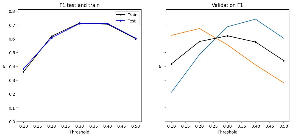
One of the main challenges was dealing with different sampling frequencies. Before moving onto the human dataset, it was necessary to make sure that the models could handle a lower sampling frequency (1024 vs 1250). There were two functions in the original code, retrain_model and prepare_training_data, which had to be altered to allow this to happen. After retraining the models to incorporate the lower sampling rate, they maintained the same strong performance as expected, as displayed in Figure 7.
Another challenge was formatting the human data. The human data was tagged differently than the mouse data. The models required a series of timestamps of SWR start and end times for ground truth data. However, the human ground truth events were represented by a continuous set of zeros and ones in each individual channel for negative and positive predictions respectively. Therefore, new code had to be written to reformat the ground truth events, shown in Figure 4. Additionally, the human data contained nine channels when the maximum number accepted by the models is eight, so one channel had to be chosen to be left out.
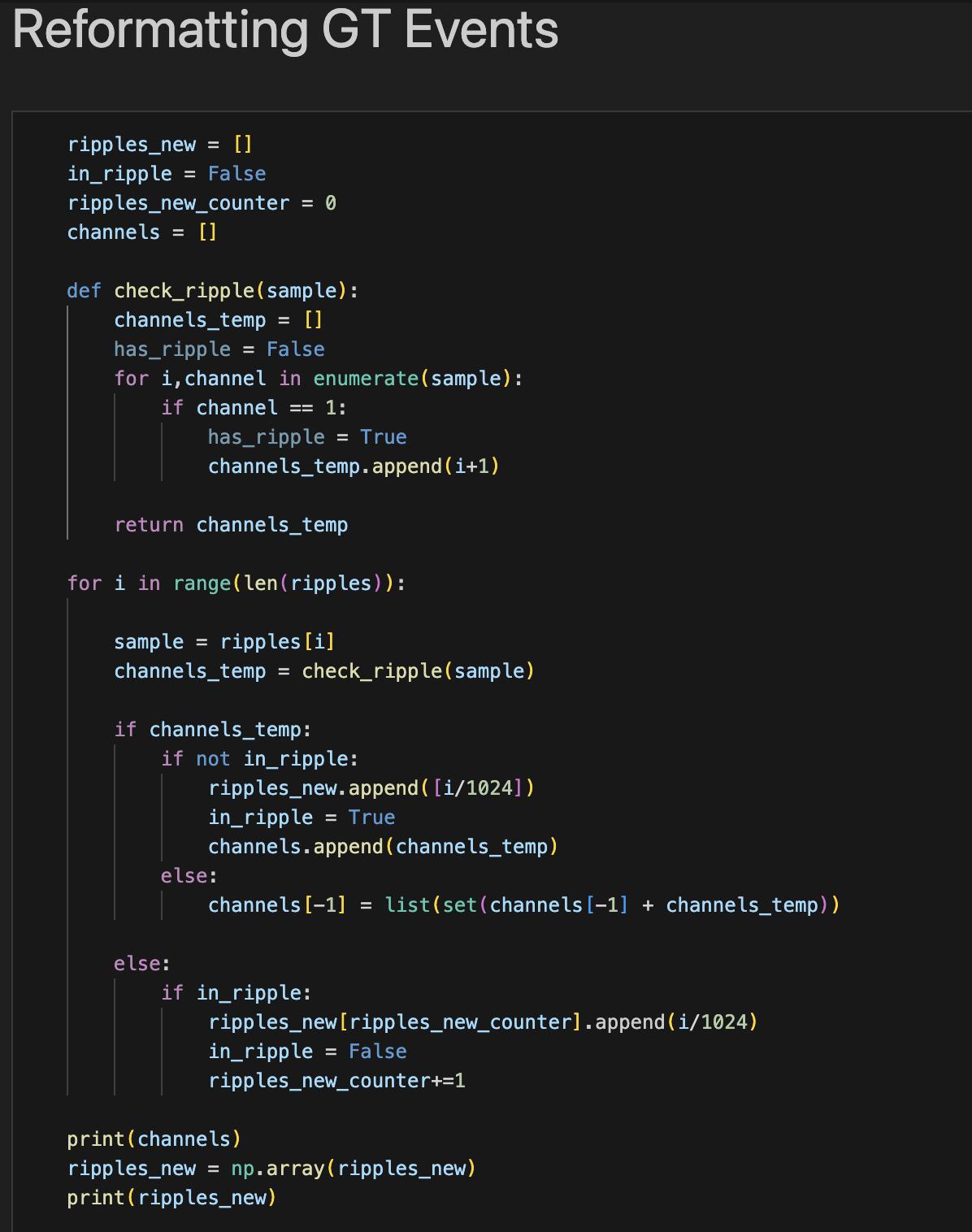
Figure 4: Python script written to reformat human ground truth events into start and stop times of SWR events.
Results

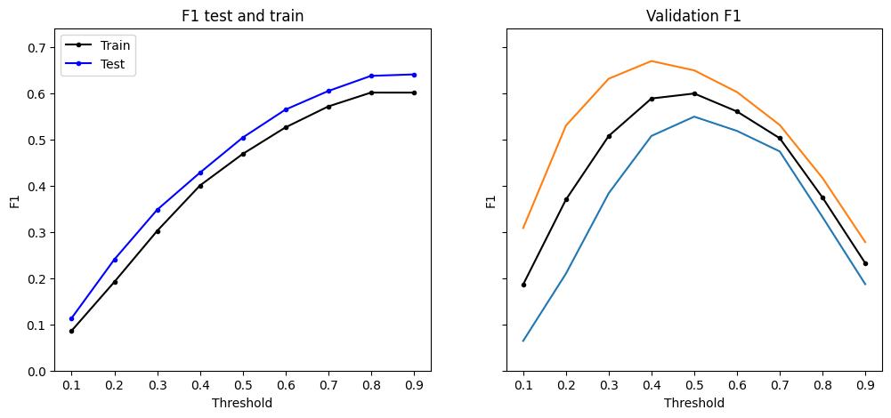
Figure 5: ML accurately detects SWR in rodent dataset (1250 Hz). The first step was validating that the models worked and all the packages had been installed correctly by testing the Prida Lab’s original models on their example rodent dataset.

Figure 6: Original models do not perform well on downsampled mouse data (1024 Hz). The challenge with sampling frequencies was brought to light when the original models were tested on manually downsampled rodent data, proving that retraining was necessary.


XGBOOST
Figure 7: Retrained models perform well on downsampled data (1024 Hz). After retraining the models, they had to be validated once again on the downsampled rodent data, before moving to human data.

Figure 8: Retrained models applied to human data. The preliminary results show XGBoost’s F1 score peaking at 0.2 with a low threshold and decline as the threshold increased, SVM performing better with low and high thresholds, LSTM having a quick spike at a threshold of 0.4, CNN2D performing relatively well over all thresholds, and CNN1D not showing any results.
Discussion
The models tested in this study performed less effectively on human data compared to rodent data. While they were somewhat effective in detecting SWRs, they would require more work to be useful. A key factor for this could have been the use of EEG data for humans versus higher resolution LFP data for rodents, which caused more noise and less precision. Additionally, the biological differences between human and rodent hippocampi likely make it harder for the models to generalize across species. Errors in data formatting of the ground truth events or parameter selection might have also contributed, especially in the CNN1D model, where predictions failed entirely. Resolving these issues involved significant adjustments to the code, such as adapting the models to handle the lower sampling rate of the EEG data and reformatting the ground truth events to align with the model’s requirements. While these adjustments allowed the models to function, they may not have been optimal for the models to perform to the best of their ability. Among the models, XGBoost and CNN2D performed the best on human data, with peak F1 scores of roughly 0.2 and 0.18. XGBoost handled the non-linear data effectively and CNN2D was able to process spatial and temporal patterns. However, other models like CNN1D require further work to be useful in this context. Future directions for this work could involve retraining the models with human specific data to better account for the characteristics of EEG data. Introducing a third category in the classifiers, to account for spike ripples, could also improve the models.
Conclusion
This study evaluated the performance of machine learning models originally developed for rodent LFP data in detecting SWRs in human EEG recordings. While the models originally showed promise in evaluating rodent and non-human primate data, the work here highlights the challenges of adapting machine learning models across species and data types. Future work could include retraining with human data and adding spike ripples as a category in the classifiers.
These findings have important implications for the field of neuroscience. By improving the detection of SWRs and SRs, machine learning models could enable more precise identification of epileptogenic zones, improve surgical outcomes, and reduce cognitive risks for patients with drug-resistant epilepsy. Beyond epilepsy, this work contributes to a broader understanding of these biomarkers and their role in memory and cognition.
References
Buzsáki, G. (2015). Hippocampal sharp wave‐ripple: A cognitive biomarker for episodic memory and planning. Hippocampus, 25(10), 1073–1188. https://doi.org/10.1002/hipo.22488
Chen, T., & Guestrin, C. (2016). XGBoost: A Scalable Tree Boosting System. Proceedings of the 22nd ACM SIGKDD International Conference on Knowledge Discovery and Data Mining, 785–794. https://doi.org/10.1145/2939672.2939785
Cortes, C., & Vapnik, V. (1995). Support-vector networks. Machine Learning, 20(3), 273–297. https://doi.org/10.1007/BF00994018
Csicsvari, J., Hirase, H., Mamiya, A., & Buzsáki, G. (2000). Ensemble Patterns of Hippocampal CA3-CA1 Neurons during Sharp Wave–Associated Population Events. Neuron, 28(2), 585–594. https://doi.org/10.1016/S08966273(00)00135-5
Joo, H. R., & Frank, L. M. (2018). The hippocampal sharp wave–ripple in memory retrieval for immediate use and consolidation. Nature Reviews Neuroscience, 19(12), 744–757. https://doi.org/10.1038/s41583-018-0077-1
Kramer, M. A., Ostrowski, L. M., Song, D. Y., Thorn, E. L., Stoyell, S. M., Parnes, M., Chinappen, D., Xiao, G., Eden, U. T., Staley, K. J., Stufflebeam, S. M., & Chu, C. J. (2019). Scalp recorded spike ripples predict seizure risk in childhood epilepsy better than spikes. Brain, 142(5), 1296–1309. https://doi.org/10.1093/brain/awz059
Leonard, T. K., Mikkila, J. M., Eskandar, E. N., Gerrard, J. L., Kaping, D., Patel, S. R., Womelsdorf, T., & Hoffman, K.
L. (2015). Sharp Wave Ripples during Visual Exploration in the Primate Hippocampus. The Journal of Neuroscience, 35(44), 14771–14782.
https://doi.org/10.1523/JNEUROSCI.0864-15.2015
Lopes da Silva, F. (2013). EEG and MEG: Relevance to Neuroscience. Neuron, 80(5), 1112–1128. https://doi.org/10.1016/j.neuron.2013.10.017
Mathon, B., Bielle, F., Samson, S., Plaisant, O., Dupont, S., Bertrand, A., Miles, R., Nguyen‐Michel, V., Lambrecq, V., Calderon‐Garcidueñas, A. L., Duyckaerts, C., Carpentier, A., Baulac, M., Cornu, P., Adam, C., Clemenceau, S., & Navarro, V. (2017). Predictive factors of long‐term outcomes of surgery for mesial temporal lobe epilepsy associated with hippocampal sclerosis. Epilepsia, 58(8), 1473–1485.
https://doi.org/10.1111/epi.13831
Navas-Olive, A., Rubio, A., Abbaspoor, S., Hoffman, K. L., & De La Prida, L. M. (2024). A machine learning toolbox for the analysis of sharp-wave ripples reveals common waveform features across species. Communications Biology, 7(1), 211. https://doi.org/10.1038/s42003-02405871-w
Pang, C.C., Kiecker, C., O'Brien, J.T., Noble, W., & Chang, R.C. (2018). Ammon’s Horn 2 (CA2) of the Hippocampus: A Long-Known Region with a New Potential Role in Neurodegeneration. The Neuroscientist, 25, 167 - 180.
Reichinnek, S., Künsting, T., Draguhn, A., & Both, M. (2010). Field Potential Signature of Distinct Multicellular Activity Patterns in the Mouse Hippocampus. The Journal of Neuroscience, 30(46), 15441–15449. https://doi.org/10.1523/JNEUROSCI.2535-10.2010
Schmidhuber, J. (2015). Deep learning in neural networks: An overview. Neural Networks, 61, 85–117. https://doi.org/10.1016/j.neunet.2014.09.003