Optimization in operations research 2nd edition rardin solutions manual by brenda.mahajan576

Optimization in Operations Research 2nd

Full chapter download at: https://testbankbell.com/product/optimizationin-operations-research-2nd-edition-rardinsolutions-manual/

Chapter 2 Solutions

proﬁt), s.t. 5x1 + 5x2 ≤ 300 (legs), 0.6x1+ 1.5x2 ≤ 63 (assembly hours), x1 ≤ 50 (wood tops), x2 ≤ 35 (glass tops), x1 ≥ 0, x2 ≥ 0

optimal

= (17 5, 35)

x = (30, 30) to

2-2 (a) max 11x1+ 17x2 (max total return), s.t. x1 + x2 ≤ 12 ($12 million investment), x1 ≤ 10 (max $10 million domestic), x2 ≤ 7 (max $7 million foreign),

x1 ≥ 5x2 (domestic at least half foreign),

x2 ≥ .5x1 (foreign at least half domestic),

x1 ≥ 0, x2 ≥ 0 (b) x ∗=domestic=$5 million,

2 = foreign=$7 million

x1 ≤ 40 (at most 40 thousand from Squawking Eagle), x2 ≤ 30 (at most 30

1Supplement to the 2nd edition of Optimization in Operations Research, by Ronald L. Rardin, Pearson

1 1 © 2017 Pearson Education, Inc., Hoboken, NJ. All rights reserved. This material is protected under all copyright laws as they currently exist. No portion of this material may be reproduced, in any form or by any means, without permission in writing from the publisher. copyright as 1 1 x ∗ x 1 ≥ 0 x 1 ≥ 0 x 1 ≤ 50 x 1 ≤ 50 x 1 ≥ 0 x 1 ≥ 0 x 1 ≤ 10 x 1 ≤ 10

1 2

(c) 12 8 x2 x 2 ≤ 7 optimal solutio n (x* 1, x* 2)=(5,7) 1 2 (c) x2 50 4 x 2 ≥ 0 40 x2≤35 30 20 ( x *, x2*) = (30,30) (d) x2 12 10 (d) x2 x2 ≥ 0 10 20 30 40 50 8 x 2 ≤ 7 4 optima 50 40 x2≤35 alternative optima x 2 ≥ 0 4 8 12 30 All optimal from x = (5, 7) to x =

20 10 x2 ≥ 0 10 20 30 40 50

(8, 4).

All

from

2-3 (a) min 3x1 + 5x2 (min total cost), s t. x1 + x2 ≥ 50 (at least 50

thousand acres),

Higher Education, Hoboken NJ, c 2017. thousand from Crooked Creek), x1 ≥ 0, x2 ≥ 0 (b) x ∗=Squawking Eagle=40

2As of September 24, 2015 thousand, x ∗=Crooked Creek=10 thousand

1 2

2 2 © 2017 Pearson Education, Inc., Hoboken, NJ. All rights reserved. This material is protected under all copyright laws as they currently exist. No portion of this material may be reproduced, in any form or by any means, without permission in writing from the publisher. copyright as

3 3 © 2017 Pearson Education, Inc., Hoboken, NJ. All rights reserved. This material is protected under all copyright laws as they currently exist. No portion of this material may be reproduced, in any form or by any means, without permission in writing from the publisher. copyright as 1 x ∗ x 1 ≤ 40 x 1 ≤ 40 x 2 ≤ 0 x x x x (c) x2 x1 + x2 ≥ 125 (weight at least 125), 2 5x1+ 1 8x2 ≤ 350 (calories at most 350), 100 x1 ≥ 0 0 2x1 + 0 1x2 ≤ 15 (fat at most 15), 3.5x1+ 2.5x2 ≤ 360 (sodium at most 360), 75 x1 ≥ 0, x2 ≥ 0 (b) x ∗=beef=25g, 2=chicken=100g 50 x 2 ≤ 30 25 x 2 ≥ 0 1 25 50 75 (d) x2 100 optimal solution (x* 1 x* 2 ) = (40,10) (c) x2 75 175 50 x 2 ≤ 30 25 150 125 max 100 x1 25 50 75 x 1 ≥ 0 75 optimal solution 50 (x* 1 x* 2) = (25,100) Improves forever in direction Δx1 = 1, 25 x 2 ≥ 0 1 Δx2 = 1. (e) x2 (d) x2 10 20 30 40 50 100 x1 ≥ 0 175 75 150 125 50 x 2 ≤ 30 25 100 75 x 1 ≥ 0 x 2 ≥ 0 50 1 25 50 75 25 x2 = 0 leaves no

2-4. (a) max x1 (max beef content), s.t. x 2 ≥ 0 1 10 20 30 40 50 x1 + x2 ≥ 200 leaves no feasible.

feasible.

2-5 (a) max 450v + 200c (max total proﬁt), s.t 10v + 7c ≤ 70000 (water at most 70000 units), v + c ≤ 10000 (total acreage 10000), v ≤ 7000 (at most 70% vegetables), c ≤ 7000 (at most 70% cotton), v ≥ 0, c ≥ 0 (b) v

= 7000, c ∗ = 0

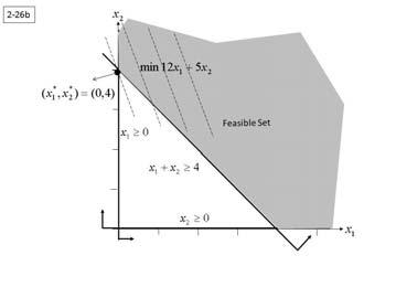
2-6. (a) min x1 + x2 (min used stock), s.t. 5x1 + 3x2 ≥ 15 (cut at least 15 long rolls), 2x1 + 5x2 ≥ 10 (cut at least 10 short rolls), x1 ≤ 4 (at most 4 times on pattern 1), x2 ≤ 4 (at most 4 times on pattern 2), x1,x2 ≥ 0 and integer (b) Partial cuts make no physical sense because all unused material is scrap. (c)

4 4 © 2017 Pearson Education, Inc., Hoboken, NJ. All rights reserved. This material is protected under all copyright laws as they currently exist. No portion of this material may be reproduced, in any form or by any means, without permission in writing from the publisher. copyright as v ≥ 0 c ≤ 7000 v ≥ 0 c ≤ 7000 (e) x2 175 (d) c 10000 150 8000 125 6000 100 4000 2000 75 50 max v 2000 4000 6000 8000 25 x1 10 20 30 40 50 Improve forever in direction Δx1 = 1, Δx2 = 2. Improves forever in direction Δv = 10, Δc = 7. (e)

∗

c 10000 8000 6000 4000 v ≤ 7000 2000 c ≥ 0 2000 4000 6000 8000 No solution with v + c = 10000. (c) c 10000 8000 6000 4000 2000 v ≤ 7000 c ≥ 0 v 2000 4000 6000 8000

optimal solution (v *, c *) = (7000,0) Either x ∗ ∗ ∗ ∗ 1 = x2 = 2, or x1 = 3, x2 = 1

(e) Both (2, 2) and (3, 1) are feasible and lie on the best contour of the objective.

2-7 (a) min 16x1+ 16x2 (min total wall 80 area), s.t. x1x2 = 500 (500 sqft pool), x1 ≥ 2x2 (length at least twice width), 60 x2 ≤ 15 (width at most 15 ft), x1 ≥ 0, x2 ≥ 0

(b) x

=length=33 1 feet, x ∗=width=15 feet

3 2 (c)

x1 ≤ 50 leaves no feasible. 2-9

x1 ≤ 25 leaves no feasible.

2-8. (a) max x2 (max number of ﬂoors), s.t π/4(x1)2x2= 150000 (150000 sqft ﬂoor space), 10x2 ≤ 4x1 (height at most 4 times diameter), x1 ≥ 0, x2 ≥ 0 (b) x ∗ = diameter

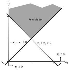
(b) min x2 (c) min x1 + x2 (d) max x2 (e)

x2 ≤ 1/2 2-10

5 5 © 2017 Pearson Education, Inc., Hoboken, NJ. All rights reserved. This material is protected under all copyright laws as they currently exist. No portion of this material may be reproduced, in any form or by any means, without permission in writing from the publisher. copyright as 2

x 1 ≥ 0 x 1 ≥ 0 x 1 ≥ 0 x 1 ≤ 25 x 1 ≤ 4 x 1 ≥ 0 x 1 ≥ 0 max x 1 ≤ 50 (d) x2 5 x 2 ≤ 4 4 3 = 78 16 feet, x ∗ = ﬂoors = 31 26 (c) x2 80 60 2 alternative optima 1 x1 1 2 3 4 5 40 20 x 2 ≥ 0 optimal solution x1

x2 20 40 60 80 100

(d)

∗

x2 40 20 x 2 ≥ 0 x 20 40 60 80 100 30 20 x 2 ≤ 15 10 optimal solution

(d) x2 x 2 ≥ 0 10 20 30 40 50 (a) 40 30 20 x 2 ≤ 15 10 x 2 ≥ 0 10 20 30 40 50

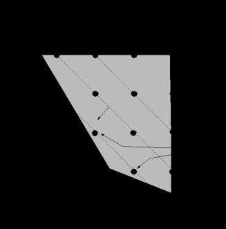
(b) min x1 + x2 (c) min x1 (d) max x1 (e)

x1 + x2 ≤ 1

2-11 (a) min 4 2 j=1 yi,j

(b) max 4

2-14. (a)

9 i=1 i=1 i=3 i

j=1 xi,j,t ≤ pi, i = 1,... , 47; t = 1,..., 10; 470 constraints

(b) 0 25 47 9 j=1 xi,j,t ≤ 47 xi,4,t; t =

1,... , 5; 5 constraints

1,... , 9; t = 1,... , 10; 4230 constraints

2-15 model; param m; param n; param q; set plots := 1 m; set crops :=

1 .. n; set years := 1 .. q; param p {i in plots }; var x{i in plots, j crops, t in years} >= 0; subject to # part (a) acrelims {i in plots, t in years }:

sum {j in crops } x[i,j,t] <= p[i];

iyi,3 αiyi 4 δiyi

4 j=1 4 j=1 yi,j = si, i = 1,... , 3

aj,iyj = ci, i = 1,... , 3

2-12. (a)

i=1 xi j t ≤ 200, j = 1,..., 5; t = , 7; 35 constraints

5 j=1 (c)

7 t=1 x5,j,t ≤ 4000; 1 constraint

j=1 xi,j,t ≥ 100, i = 1,..., 17; t = 1,... , 7;

119 constraints

2-13 model; param m; param n; param

p; set products:= 1 m; set lines := 1 n; set weeks := 1 p; var

x{i in products, j in lines,t in weeks} >= 0; subject to

# part (a)

linecap {j in lines, t in weeks}: sum {i in products} x[i,j,t] <= 200;

# part (b)

prod5lim: sum {j in lines, t in weeks} x[5,j,t] <= 4000;

# part (c)

minprodn{i in products, t in weeks}: sum {j in lines} x[i,j,t] >= 100;

# data; param m := 17; param n := 5; param p := 7;

# part (b)

crop4min {t in years: t <= 5 }:

0.25* sum {i in plots, j in crops }

x[i,j,t] <= sum {i in plots } x[i,4,t]; # part (c)

beam1st {i in plots, j in crops, t in years}: x[i,1,t] >= x[i,j,t]; #

data; param m := 47; param n := 9; param q := 10;

because LHS is a weighted sum of the decision variables. (b) Linear because both LHS and RHS are weighted sums of the decision variables (c) Nonlinear because LHS has reciprocal 1/x9 (d) Linear because LHS is a weighted sum of the decision variables (e) Nonlinear because LHS has (xj)2 terms. (f) Nonlinear because LHS has log(x1) term, and RHS has a product of

6 6 © 2017 Pearson Education, Inc., Hoboken, NJ. All rights reserved. This material is protected under all copyright laws as they currently exist. No portion of this material may be reproduced, in any form or by any means, without permission in writing from the publisher. copyright as

(e) (f) 17 (b)

(a)

2-16. (a) f(y1,y2, y3) = Δ (y1)2y2/y3, g1(y1, y2, y3) = Δ y1 + y2 + y3, b1 = 13, g2(y1, y2, y3) = Δ 2y1 y2 + 9y3, b2 = 0, g3(y1, y2, y3) = Δ y1, b3 = 0, g4(y1, y2, y3) = Δ y3, b4 = 0 (b) f(y1,y2, y3) = Δ 13y1 +22y2 +10y2y3 +100, g1(y1, y2, y3) = Δ y1 y2 + 9y3, b1 = 5, g2(y1, y2, y3) = Δ 8y2 4y3, b2 = 0, g3(y1, y2, y3) = Δ y1, b3 = 0, g4(y1, y2, y3) = Δ y2, b4 = 0, g5(y1, y2, y3 = Δ y3, b5 = 0, 2-17.

Linear

(a)

variables (g) Nonlinear because LHS has max operator.(h) Linear because LHS is a weighted sum of the decision variables.

2-18. (a) LP because the objective and all constraints are linear. (b) NLP because of the nonlinear objective function with reciprocal of w2. (c) NLP because of the nonlinear ﬁrst constraint.(d) LP because the objective and all constraints are linear.

2-19. (a) Continuous because fractions make sense. (b) Discrete because they either closed or not. (c) Discrete because a speciﬁc process must be used. (d) Continuous because fractions can probably be ignored.

2-24 (a) Model (d) because LP’s are generally more tractable than ILP’s. (b) Model (d) because LP’s are generally more tractable than NLP’s (c) Model (d) because LP’s are generally more tractable than INLP’s. (d) Model (f) because ILP’s are generally more tractable than INLP’s. (e) Model (g) because LP’s are generatlly more tranctable than ILP’s.

(service NE), y1 + y2 + y3 ≥ 1 (service SE), yj = 0 or 1, j = 1,... , 4 (b) Build 3 and 4, i.e. y ∗ = y ∗ = 0, y ∗ = y ∗ = 1

2-23 (a) ILP because the objective and all constraints are linear, but variables are discrete.(b) NLP because the objective is nonlinear and all variables are continuous (c) INLP because the objective is nonlinear and variables are discrete. (d) LP because the objective and all constraints are linear, and all

the one constraint is nonlinear, and z3 are discrete. (f) ILP because the objective and all constraints are linear, but variables z1 and z3 are discrete (g) LP because the objective and all constraints are linear, and all variables are continuous. (h) INLP because the objective is nonlinear and z3 is discrete.

7 7 © 2017 Pearson Education, Inc., Hoboken, NJ. All rights reserved. This material is protected under all copyright laws as they currently exist. No portion of this material may be reproduced, in any form or by any means, without permission in writing from the publisher. copyright as x 1 ≥ 0 x 1 ≥ 0 x 1 ≤ 8 x 1 ≤ 8

2-25. (a) x2 j=1 16 x1 + x2 + x4 + x5 ≥ 2 (c) x3 + x8 ≤ 1 (d) (max total score), s t. 700x1+ 400x2+ 300x3+ 600x4 ≤ 1000 ($1 (b) Fund 2 and 4, i.e. x ∗ = x ∗ = 0, 12 8 4 max alternative optimal solutions 1 3 2 = x4 = 1

y3 + 35y4

total

y4 ≥

x 2≥ 0 x1 4 12 16 Alternative optima from x ∗ ∗ NW), y1

y1 + y4 ≥ 1 x1 = 8, x2 = 12 1 = 8, x2 = 0 to

2-22 (a) min 43y

+ 175

+ 60

(min

land cost), s.t. y

1 (service

+ y2 + y4 ≥ 1 (service SW),

+ y3 ≥ 1 (service capital),

∗ ∗ (b) x2 16 12 8 4

x 2 ≥ 0 x1 4 12 16 optimal solution (x* 1 , x* 2 ) = (0,4) Unique optimum x1 = 0, x2 = 4 (c) Helping ∗ ∗ one can hurt the other. 2-26

(a) x2 + x5 + x8 ≤ 2500 (well 2), x3 + x6 + x9 + x10 ≤ 7000 (well 3)

(e) xj ≤ uj, j = 1,... , 10 10

(f)

(g) xj ≥ 0, j = 1,... , 10

(h) A single objective LP because the one objective and all constraints are linear, and all variables are continuous.

(i)

2-29 (a) The decisions to be made are which projects to undertake.

(b) pj = Δ the proﬁt for project j, mj = Δ the man-days required on project j, and tj = Δ the CPU time required on project j

(d) 7 ≤ 8 pjxj mj xj /240 ≤ 10 8 j=1

j=1 tj xj ≤ 1000 (computer time), Unique

j=1 xj ≥ 3 (select at least 3); x3 + x4 + x5 + x8 ≥ 1 (include at least 1 of director’s favorites)

(f) xj = 0 or 1, j = 1,... , 8

(g) A single objective ILP because the one objective and all constraints are linear, but variables are discrete. 2-27. (a) min

= x6 = x7 = 1, others = 0

2-30. (a) We must decide what quantities to move from surplus sites to fulﬁll each need.

(b) si = Δ the supply available at i, rj = Δ the quantity needed at j, di,j = Δ the distance from i to j. 1600 (at most 1600 Ohms resistance), 00175x4 + 00130x5 + 00161x6 + 00095x9 + (c) min 4 7

(d) j=1 xi,j = si, i = 1,... , 4 attenuation),

00048x12 ≤ 8 5 (at most 8.5 dBell

(e) 4 i,j j i=1 x = r , j = 1,... , 7 x4,x5,x6,x9,x12 ≥ 0

(b) Nonzeros: x ∗ = 1000, x ∗ = 15000

(f) xi,j ≥ 0, i = 1,... , 4, j = 1,..., 7

(g) A single objective LP because the one 5 12

2-28. (a) Pump rates are the decisions to be made.

(b) uj= Δ the capacity of pump j, cj= Δ the

objective and all constraints are linear, and all variables are continuous.

(h) Nonzeros: x ∗ 1 = 81, x ∗ 2 = 93,

(d) x1 + x4 + x7 ≤ 3000 (well 1), 2-31

(a) The values to be chosen are the

8 8 © 2017 Pearson Education, Inc., Hoboken, NJ. All rights reserved. This material is protected under all copyright laws as they currently exist. No portion of this material may be reproduced, in any form or by any means, without permission in writing from the publisher. copyright as

i=1

=1 (e) 8

j=1 xj ≥ 10000

x ∗ = x ∗ = x ∗ =

x ∗ = x ∗ = 1500, 1 2 3 x ∗ ∗ 4 6 ∗ ∗ ∗ 5 =

Unique optimum x ∗ = 4, x ∗ = 0 1 2

1100,

1400, x7

400¡ x8

x10

0, x9 = 1900

(b)

optimum x ∗ = 0, x ∗ = 4 (c) Helping 1 2 one can hurt the other.

(h) x ∗ ∗ ∗ ∗

s.t

.092x4 + .112x5+ .141x6+ .420x9 + .719x12 (min total cost),

x4 + x5 + x6 + x9 + x12 = 16000 (16000m line), .279x4+ .160x5+ .120x6+ .065x9+ .039x12 ≤

= x3

j=1 di j xi j

pumping cost of

x ∗ 3 1, 1,5 1, 1,6 1,7 1, = 166, x ∗ = 90, x ∗ = 85, x ∗ = 145,

pump j

cj xj x ∗ 2 =

x ∗ 1 = 166, x ∗ = 105, x ∗

j=1 2, 3, 3,4 4,3

301,

= 99

coeﬃcients in the estimating relationship.

(b) Relatively large values can be rounded if

k/(1 + ea+bfj ) (min fractional without much loss, and continuous total squared error)

(b) min

2-32 (a) The decisions to be made are where to assign each teacher.

(b)

(min total cost),

is more tractable.

(c) ci,j = Δ the cost of moving a car from i to j, pj = Δ the number of cars presently at j, nj = Δ the number of cars required at j

(max (g) A single objective LP because the one total supervisor preference), max objective and all constraints are linear, and

j=1 pi,j xi,j (max total principal all variables are continuous.

4,2 = 115, x4,3 = 165,

22 xi,j = 1, i = 1,... , 22 (each teacher x5,1 = 85, x5,3 = 225

22 xi,j = 1, j = 1,... , 22 (each school

(e) xi,j = 0 or 1, i, j = 1,... , 22

(f) A multiobjective ILP because the 4 objectives and all constraints are linear, but variables are discrete.

2-33 (a) Each task must go to Assistant 0 or Assistant 1

(b) max 100(1 x1) + 80x1 + 85(1 x2) +

70x2 + 40(1 x3) + 90x3 + 45(1 x4) +

85x4+ 70(1 x5) + 80x5+ 82(1 x6) + 65x6

2-36 (a) We must decide how much of what fuel to burn at each plant

min 4 23 p=1 cf,pxf,p

(d) 4 ef xf,p ≥ rp, p = 1,... , 23 (each plant p); 23 constraints

(e) xf,p ≥ 0, f =1,... , 4, p = 1,... , 23; 92 constraints

(f) A multiobjective LP because the 2 objectives and all constraints are linear, and all variables are continuous.

2-37 (a) The available options are to buy 6 j=1 xj = 3 whole logs or green lumber.

(d) x5 = x6

(e) xj = 0 or 1, j = 1,... , 6

(f) A single objective ILP because the one objective and all constraints are linear, but variables are discrete

(g) x ∗ = x ∗ = x ∗ = 1, others = 0 2 3 4

2-34 (a) Batch sizes are the decisions to be made.

(b) min xj /dj , j = 1,... , 4 (each burger j)

(b) Relatively large magnitudes can be rounded without much loss, and continuous is more tractable.

70x10 + 200x15+ 620x20+ 1 55y1 + 1 30y2

(d) 100( 09)x10+ 240( 09)x15+ 400( 09)x20+

10y1 + 08y2 ≥ 2350

(e) x10 + x15 + x20 ≤ 1500 (sawing capacity), 100x10+ 240x15+ 400x20+ y1 + y2 ≤ 26500

4 j=1 tj dj /xj ≤ 60 (drying capacity)

(d) 0 ≤ xj ≤ uj, j = 1,... , 4

(e) Multiobjective NLP because the ﬁrst

9 9 © 2017 Pearson Education, Inc., Hoboken, NJ. All rights reserved. This material is protected under all copyright laws as they currently exist. No portion of this material may be reproduced, in any form or by any means, without permission in writing from the publisher. copyright as j=1 i=1 c i=1 max 22 i=1 22 f=1 f=1 (c) (c)

n cj

(d) min 5 (e) 5 5 j=1,j=i 5 i,j xi,j

min

i=1,i=k xi,k j=1,j=k xk,j = nk pk, k = 1,... , 5 (each region k) 22 i=1 j=1 ti,j

i,j

(f) xi,j ≥ 0, i, j = 1,... , 5, i = j preference), max 22

j=1

22 i

(h) Nonzero values: x ∗ ∗ preference)

∗ ∗ j

(d)

22 22

=1 ci,j xi,j

(max total teacher

si,j

i,j

(c)

)

(b)

)

constraint is nonlinear and all variables are continuous.

2-35

(a) The issue is how many cars to move from where to where

(f) x10 ≤ 50 (size 10 log availability), x15 ≤ 25 (size 15 log availability), x20 ≤ 10 (size 20 log availability), y1 ≤ 5000 (grade 1 green lumber availability)

(g) x10,x15,x20,y1, y2 ≥ 0

(h) A single objective LP because the one

1 0 10 © 2017 Pearson Education, Inc., Hoboken, NJ. All rights reserved. This material is protected under all copyright laws as they currently exist. No portion of this material may be reproduced, in any form or by any means, without permission in writing from the publisher. copyright as

objective and all constraints are linear, and all variables are continuous.

states := 1 n; var x{i in sites, j in states } >= 0; var y{i in sites }

(i) x ∗ = 50, x ∗ = 25, x ∗ = 5, y ∗ = 5000, binary; param c {i in sites, j in i in sites }

2 = 8500

2-38 (a) Decisions to be made are when to schedule each ﬁlm.

binary; param r { j in states }; minimize totcost: sum{i in sites, j

(b) min m 1 m aj,j n xj,txj ,t in states} c[i,j]*r[j]*x[i,j] + sum{i

n t=1 m j=1

j=1 j =j+1 t=1

xj,t = 1, j = 1,.. ,m (each ﬁlm j)

xj,t ≤ 4, t = 1,.. ,n (each time t)

(e) xj,t = 0 or 1, j = 1,.. ,m; t = 1,.. ,n

(f) A single objective INLP because the one objective is nonlinear, and variables are discrete. (g) model; param m; param n; set films := 1 m; set slots := 1 n; var x{j in films,t in slots }

binary; param a{ j in films, jp in films }; minimize totconflict: sum{ j in films, jp in films: j < m and jp >

in sites}f[i]*y[i]; x[j,t]*x[jp,t]; subject to doeach{j in states}: sum{i in sites}x[i,j] = 1; switch {i in

sites, j in states }: x[i,j] <= y[i]; data; param m := 5; param n := 5;

j } a[j,jp]*sum {t in slots} 2-40 (a) max 8 rj xj, subject to, x[j,t]*x[jp,t]; subject to allin {j in films}: sum{ t in slots } x[j,t] = 1; max4 {t in slots}:sum{j in films} x[j,t] <= 4;

2-39 (a) We need to decide both which oﬃces to open and how to service customers from them.

(b) Oﬃces must either be opened or not.

j=1 xj ≤ 4, x1 + x2 + x3 ≥ 2, x4 + x5 + x6 + x7 + x8 ≥ 1, x2 + x3 + x4 + x8 ≥ 2, x1 x8 = 0 or 1 (b) model; param n ; set games := 1 n; #ratings param r{j in games}; #home? param h{j in games}; #state? param s{j in games}; #cover? var x{j in games} binary; maximize totrat: sum{j in games} r[j]*x[j]; subjectto capacity: sum{j in games} x[j] <= 4; home: sum{j in games} h[j]*x[j] >= 2;

(d) min 5 5 j=1 ci j rjxi j + 5 fiyi away: sum{j in games}(1-h[j])* x[j] >= 1; state: sum{j in games}s[j]*x[j] 5 i=1

j) xi,j = 1, j = 1,... , 5 (each location >= 2; data; param n := 8; param r :=1

(f) xi,j ≤ yi, i, j = 1,... , 5 (each site i, location j combination)

(g) xi j ≥ 0, i, j = 1,... , 5, yi = 0 or 1, i = 1,... , 5

(h) A single objective ILP because the one objective and all constraints are linear, but the yi variables are discrete.

(i) Nonzeros:

The model is an ILP because all constraints and the objective are linear, but decision variables are binary

2-41 (a) How to divide funds is the issue.

1 1 11 © 2017 Pearson Education, Inc., Hoboken, NJ. All rights reserved. This material is protected under all copyright laws as they currently exist. No portion of this material may be reproduced, in any form or by any means, without permission in writing from the publisher. copyright as 10

20 1 y ∗ (c) (d) j=1 8 i=1 i=1 (e) j=1

f := 1 160 2 49 3 246 4 86 4 100; param r := 1 200 2 100 3 300 4 100 5 200; param c: 1 2 3 4 5 := 1 0.0 0.4 0.8 0.4 0.8 2 0.7 0.0 0.8 0.4 0.4 3 0.6 0.4 0.0 0.5 0.4 4 0.6 0.4 0.9 0.0 0.4 5 0.9 0.4 0.7 0.4 0.0 ;

param

3.0 2 3.7 3 2.6 4 1.8 5 1.5 6 1.3 7

1.6 8 2.0; param h:=1 1 2 1 3 1 4 0 5 0 6 0 7 0 8 0; param s:=1 0 2 1 3 1 4 1 5 0 6 0 7 0 8 1;

(c)

n vj xj x ∗ ∗ ∗ ∗ ∗ (c) min n rj xj 2,2 = x2,4 = x3,1 = x3,3 = x5,5 = 1, j=1 y ∗ ∗ ∗ n 2 = y3 =

5 =

n; set

m; set (d) j=1 xj = 1 (e) xj ≥ j , j = 1,.. ,n (each

(b) max

1 (j) model; param m; param

sites :=