~ refe reed pape r
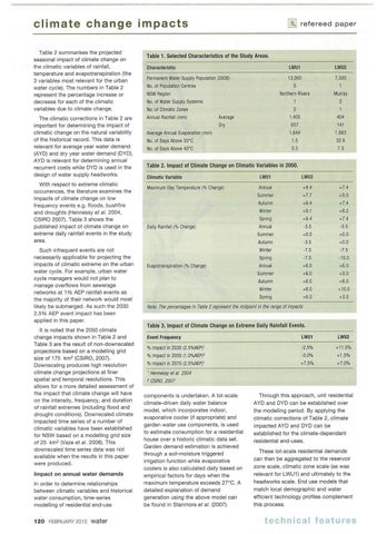
climate change impacts Table 2 summarises the projected seasonal impact of climat e change on the climatic variables of rainfall, temperature and evapotranspiration (the 3 variables most relevant for the urban water cycle). The numbers in Table 2 represent the percentage increase or decrease for each of the climatic variables due to climate change. The climatic corrections in Table 2 are important for determining t he impact of climatic change on t he natural variability of the historical record. This data is relevant for average year water demand (AYO) and dry year wat er demand (DYD). AYO is relevant for determining annual recurrent costs wh ile DYD is used in the design of water supply headworks. With respect to extreme cl imatic occurrences, the literature examines the impacts of climate change on low frequency events e.g. floods, bushfire and d roughts (Hennessy et al. 2004, CSIRO 2007). Table 3 shows the published impact of climate change on extreme daily rainfall events in the st udy area. Such infrequent events are not necessarily applicable for projecting the impacts of climatic extreme on the urban water cycle. For example, urban wat er cycle managers would not plan to manage overflows from sewerage networks at 1 % AEP rainfall events as t he majority of their network would most likely be submerged. As such the 2030 2.5% AEP event impact has been applied in this paper. It is noted that the 2050 cl imate change impacts shown in Table 2 and Table 3 are t he result of non-downscaled projections based on a modelling grid size of 175 km 2 (CSIRO, 2007). Downscaling produces high resolution climate change projections at finer spatial and temporal resolutions. This allows for a more detailed assessment of the impact that climate change wi ll have on the intensity, frequency, and duration of rainfall extremes (including flood and drought conditions). Downscaled cl imate impacted time series of a number of climatic variables have been established for NSW based on a modelling grid size of 25 km 2 0Jaze et al. 2008). This downscaled time series data was not available when the results in this paper were produced.
Impact on annual water demands In order to determine relationships between climatic variables and historical water consum ption, time-series modelling of residential end-use
120 FEBRUARY 2010
water
Table 1. Selected Characteristics of the Study Areas. Characteristic
LWU1
LWU2
Permanent Water Supply Population (2008)
13,000
7,300
No. of Population Centres
5
NSW Region
Northern Rivers
Murray
2
1
1,405
404
657
141
2
No. of Water Supply Systems No. of Climatic Zones Annual Rainfall (mm)
Average Dry
1,644
1,863
No. of Days Above 35°C
1.5
32.6
No. of Days Above 40°C
0.3
7.3
Average Annual Evaporation (mm)
Table 2. Impact of Climate Change on Climatic Variables in 2050. Climatic Variable Maximum Day Temperature (% Change)
LWU1
LWU2
Annual
+9.4
Summer
+7.7
+5.5
Autumn
+6.4 +9.1
+7.4
Annual
+9.4 -3.5
+7.4 -3.5
Summer
+0.0
+0.0
Autumn
-3.5
Winter Spring
-7.5
+0.0 -7.5
-7.5
-15.0
Annual
+6.0
+6.0
Summer
+6.0
+3.0
Autumn
+6.0
+6.0
Winter Spring
+6.0
+10.0
+6.0
+3.0
Winter Spring Daily Rainfall (% Change)
Evapotranspiration (% Change)
+7.4
+8.2
Note: The percentages in Table 2 represent the midpoint in the range of impacts
Table 3. Impact of Climate Change on Extreme Daily Rainfall Events. Event Frequency
LWU1
LWU2
% Impact in 2030 (2.5%AEP) 1
-2.5%
+11 .0%
% Impact in 2050 (1.0%AEP)2
-3.0%
+1.5%
% Impact in 2070 (2.5%AEP)1
+7.5%
+7.0%
1 Hennessy 2
et al. 2004
CS/RO, 2007
components is undertaken. A lot-scale climate-driven daily water balance model, wh ich incorporates indoor, evaporative cooler (if appropriate) and garden water use components, is used to estimate consumption for a residential house over a historic climat ic data set. Garden demand estimation is achieved throug h a soil -moisture triggered irrigation function while evaporat ive coolers is also calculated daily based on empirical factors for days when the maximum temperature exceeds 27°C. A detailed explanation of demand generation using the above model can be found in Stanmore et al. (2007).
Through this approach, unit residential AYO and DYD can be established over the modelling period . By applying the climat ic corrections of Table 2, climat e impacted AYD and DYD can be established for the climate-dependant residential end-uses. These lot-scale residential demands can then be aggregated to the reservoir zone scale, climatic zone scale (as was relevant for LWU1) and ultimately to the headworks scale. End use models that match local demographic and water efficient technology profiles complement this process.
technical features