82. We need to show a is constant: a and ks a v œœ œœœÊ œœ dv dvdvdsdvd k dvdsdv dt dtdsdtdsds dsdtds 2s
which is a constant.
œ Ê kkk 2s s ss $Î#
œœœ
# ## È # "" #
œœœœœœœ ˆ‰
w
86. The graph of y(fg)(x) has a horizontal tangent at x1 provided that (fg)(1)0 f(g(1))g(1)0œ‰œ‰œÊœ www either f(g(1))0 or g(1)0 (or both) either the graph of f has a horizontal tangent at ug(1), or the ÊœœÊœ ww graph of g has a horizontal tangent at x1 (or both). œ
ÉÈ
x x, in agreement. Êœ œœ dy dxdx4 xx d x """" ## # $Î%
ÈÈÈ
È È È ˆ‰
É "Î%
1. xyxy6: ## œ
Step 1: x y2xx2y y10Š‹Š‹ ## dydy dxdx œ
Step 2: x 2xy 2xyy ## dydy dxdx œ
Step 3: x2xy2xyy dy dx ab## œ
Step 4: dy2xyy dxx2xy œ # #
xy18xy 3x3y 18y18x
3y18x
Step 1: 2x 2y2y 1 Š‹ dy dydy dx dxdx œ
Step 2: 2x 2y 12y dydydy dxdxdx œ
Step 3: (2x2y1)2y dy dx œ"
Copyright © 2012 Pearson Education, Inc. Publishing as Addison-Wesley University Calculus Elements with Early Transcendentals 1st Edition Hass Solutions Manual Full Download:http://testbanktip.com/download/university-calculus-elements-with-early-transcendentals-1st-edition-hass-solutions-manual/ Download all pages and all chapters at: TestBankTip.com
92
81. s(4t) v(14t)(4)2(14t) v(6)2(6) m/sec; œ" Êœœ œ Êœ" %œ "Î# "Î# "Î# "Î# " # ds 2 dt 5 v2(4t)a 2(14t)(4)4(14t)a(6)4(146) m/sec œ" Êœœ œ Êœ œ "Î# $Î# $Î# $Î# # " # # dv 4 dt 15
Chapter 2 Differentiation
†† † ˆ‰ È È ks
œœ kk 2s È È # #
œ
83. v proportional to v for some constant k . Thus, a v " ÈÈ ss kdvkdvdvdsdv dsdtdsdtds 2s Êœ Êœ ˆ‰
$Î# acceleration is a constant times so a is inversely proportional to s.
84. Let f(x). Then, a f(x) f(x)(f(x))f(x)f(x)f(x), as required. dx dvdvdxdv ddx d dt dtdxdtdx dxdt dx
85. No. The chain rule says that when g is differentiable at 0 and f is differentiable at g(0), then fg is differentiable at 0 ‰ . But the chain rule says nothing about what happens when g is not differentiable at 0 so there is no contradiction.
ÉÉ ÈÈ È ˆ‰ È
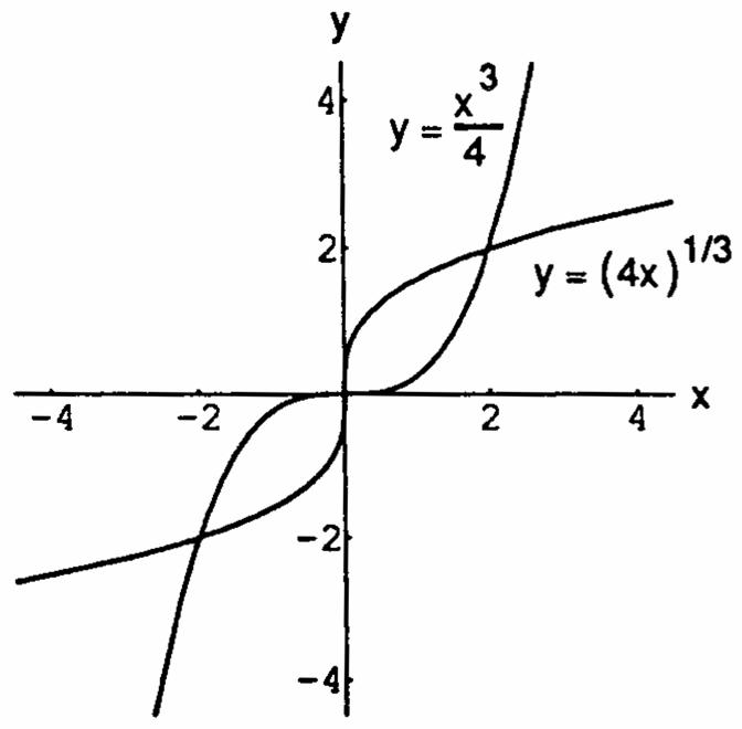
87. From the power rule, with yx, we get x. From the chain rule, yxœœœ "Î% $Î% " dy dx4
88. From the power rule, with yx, we get x. From the chain rule, yxxœœœ $Î% "Î% dy dx4 3 ÉÈ xx xx x Êœ Êœ œ œ dy dy dx dx dx xx xx xx 4xx d 3 x 3x "" " " ### # # ÉÉÉ É
ˆ‰ ÈÈ È Š‹
x, in agreement. œœ 3x 4xx 3 4 È ÈÈ
2.8 IMPLICIT DIFFERENTIATION
œ Ê œ
2.
18y3x $$ ## # # œÊ
ʜ dy dy dy dy6yx dx dx dx dxy6x ab # #
3. 2xyyxy: œ #
Step 4: dy12y dx2x2y1 œ
4. xxyy1 3xyx 3y 0 3yx y3x $$#### œÊ œÊ œ Êœ dydy dy dyy3x dxdx dx dx3yx ab # #
5. x(xy)xy: #### œ
Step 1: x2(xy)1(xy)(2x)2x2y ##
œ dy dy dx dx
Step 2: 2x(xy) 2y 2x2x(xy)2x(xy) œ ## # dydy dxdx
Step 3: 2x(xy)2y2x1x(xy)(xy) dy dx cdcd œ ##
Step 4: dy dx2x(xy)2yyx(xy)xyxy 2x1x(xy)(xy)x1x(xy)(xy) x1xxyx2xyy œœœ cd cd ab ## ### $
### œ x2x3xyxy xyxy $## #$
6. (3xy7)6y 2(3xy7)3x 3y6 2(3xy7)(3x) 6 6y(3xy7) œÊ œÊ œ #
dy dy dydy dx dx dxdx [6x(3xy7)6]6y(3xy7) Ê œ Êœ œ dy dyy(3xy7)3xy7y dx dxx(3xy7)113xy7x # #
7. y 2y # "" œÊœœÊœ x2 x1dx(x1)(x1)dxy(x1) dy(x1)(x1)dy ###
8. x xxyxy 3x2xyxy1y x1y13x2xy y #$ ### ww#w#w œÊ œ Ê œ Ê œ Êœ xy 13x2xy xy x1 ab # # 9. xtan y 1secy cosy œÊœÊœœ ab## " dydy dxdxsecy # 10. xycot xy xycsc(xy)xy xxcsc(xy)ycsc(xy)y œÊ œ Ê œ ab Š‹ dy dy dy dy dx dx dx dx ## # xxcsc(xy)ycsc(xy) Ê œ "Êœœ dy dy y dx dx x ycsc(xy) xcsc(xy) ‘ ‘ ## " " ‘
yxy
y) yx (cos yx) y1 œÊ œ Ê œ Êœ dy dy dy dyy1 dx dx dx dxcos yx
13. y sin1xy ycos(1) sin x y Š‹ ’
"" " " y y ydx ydxdx dy dydy œ Ê œ Ê # cossinxy dy dy y y dxyy y dx cossinxy sincosxy
’“ Š‹Š‹
œ Êœœ """ """ ""
# yyy yy Š‹Š‹
Š‹Š‹
14. e2x2yexy2xy22yxey2xye22yxey2y22xye xy xy2 2xy xy 2xy xy 22 2 222 œ Ê œ Ê œ Ê œ abwwwww w y Êœ w 22xye xe2 xy 2 2xy 2
15. r1 r0 )) "Î#"Î# "Î# "Î# "" " " ## # # œÊ œÊœÊœ œ † dr dr dr dd d r 2rr 2 )) ) ))) ’“ÈÈ ÈÈ ÈÈ
16. r2 œ Ê œ Êœ È ))))))))) 34 dr dr 3d d # #Î$$Î% "Î# "Î$ "Î% "Î# "Î$ "Î% ))
17. sin(r) [cos(r)]r 0 [ cos(r)]r cos(r) , )))))) œÊ œÊœ Êœœ " # ˆ‰ dr dr dr r dd d cos (r ) r cos(r) )) )))) ) cos(r)0 ) Á
Differentiation93
Section 2.8 Implicit
’“ Š‹
Š‹
11. esin(x3y) 2e13y cos(x3y) 13y 3y 1 2x 2x 2e 2e cos(x3y) cos(x3y) œ Êœ Ê œÊœ abwww 2x 2x y Êœ w 2ecos(x3y) 3 cos(x3y) 2x 12.
‘ # #
xsin
1(cos
“Š‹ Š‹
Copyright © 2012 Pearson Education, Inc. Publishing as Addison-Wesley
Chapter 2 Differentiation
18. cos rcot e sin rcsc er sin rcsc ree œÊ † œ Ê † œ ))))) rr r r dr dr dr dr dddd )) ) ) )))) ##
#
sin re recsc Ê œ Êœ dr dr drrecsc dd d rr esin r )) ) )) ) ) )) # r r ) )
19. xy1 2x2yy0 2yy2x y; now to find , y ## w w w w œÊ œÊœ Êœœ œ dy dy dx y dxdxdxy xd d x # # ab Š‹ y since y y Êœœ œ Êœœœœ ww w ww " " y(1)xy dy yx yyydxyyy yx x yy w# # # ## #$$$
## Š‹ ab x y
20. xy1 xy 0 y x y ; #Î$#Î$ "Î$ "Î$ "Î$ "Î$w "Î$ œÊ œÊ œ Êœœ œ 22 22 x 3 3dx dx3 3 dx x dy dy dy y y ‘
Differentiating again, yww œœ xyyyx xx
xyyx "Î$ #Î$w"Î$ #Î$ "" #Î$#Î$
"Î$ #Î$"Î$ #Î$ "" "Î$ "Î$ ˆ‰ˆ‰ ˆ‰ˆ‰ Œ 33 33 y x
"Î$ "Î$
"" " #Î$ "Î$"Î$ %Î$
xyyx Êœ œ dy y dx3 3 3x3yx # "Î$ # %Î$"Î$#Î$
# w ### x xxx
21. ye2x 2yy2xe2#w œ Êœ ʜʜ xx dydy dxydxy xe1 y2xeexe1y ## # # ##
œœ y2xeexe1 y2xeexe2xe1 yy Š‹Š‹Š‹Š‹ ## # ### #### # #
xxx 2xx2xx xe1 x y 3 † œ ˆ‰ 2xyy2xexe1 y #### 22x2x 3
22. y2x12y 2yy22y y(2y2)2 y(y1); then y(y1)y #w w ww " ww # w " œ Ê œ Ê œÊœœ œ y1 (y1)(y1) y œ Êœœ # " ww " dy dx (y1) # # $
23. 2yxy yy1y yy11 y ; we can
œ Êœ Ê œÊœœœ "Î#w ww "Î# w " dy dx y1 y1 y "Î# È È differentiate the equation yy11 again to find y: yyyy1y0 w "Î# www $Î#w "Î#ww " #
" #
y1yyy y Ê œÊœœœœ
cd"Î#www $Î# ww "" " # # # dy dx y y1 2yy1 1y # #
# $Î# "Î# $Î# "Î# $$ Œ ab ab ˆ‰ È
" "Î# y1
24. xyy1 xyy2yy0 xy2yyy y(x2y)y y; y œÊ œÊ œ Ê œ Êœœ #wwwww www ydy (x2y)dx # #
œœœ (x2y)yy(12y) (x2y)(x2y)(x2y) (x2y)y12 y(x2y)y(x2y)2y ww ###
# ’“’“ Š‹ cd " yy (x2y)(x2y) (x2y)
œœœ2y(x2y)2y2y2xy2y(xy) (x2y)(x2y)(x2y) ## $$$
25. xy16 3x3yy0 3yy3x y; we differentiate yyx to find y:
# ## 2 œÊœœ œ œ œ (2)(1)(0) 44 ˆ‰ " # 27. yxy2x at () and (1) 2y 2x4y 2 2y 4y 22x ##% $ $ œ #ß" #ß Ê œ Ê œ dy dy dydy dx dx dxdx 2y4y22x 1 and 1 Ê œ ʜʜ œ dy dy dy dy dx dxyydx dx x ab ¹¹ $ " # $ (21) (21) ß ß Copyright © 2012 Pearson Education, Inc. Publishing as Addison-Wesley
94
ˆ‰
ˆ‰
Š‹Š‹
È ˆ‰
ˆ‰ ˆ‰ˆ‰ œ œ
ˆ‰
$$ ##w#w#w #w#ww œÊ œÊœ Êœ œ x y # # yyy2yy2x yy2x2yy y #wwww #ww www # œ Êœ Êœœ cdcd † 2x2y 2x yy Š‹x2x yy #% #$ 2xy2xdy ydx32 3232 $%# &# ¹ (22) ß 26. xyy1 xyy2yy0 y(x2y)y y y ; œÊ œÊ œ ʜʜ #www www y (x2y) (x2y) (x2y)y(y)12y abab ww # since y we obtain y kk www"" # (01) (01) ß ß
(b) the normal line is y4(x3) yx œ Êœ 44 33
31. xy9 2xy2xyy0 xyyxy y; ## ##w #w#w œÊ œÊœ Êœ y x
(a) the slope of the tangent line my 3the tangent line is y33(x1) y3x6 œœ œÊ œ Êœ k ¸ w (13)
(b)
(a)
(b)
Š‹
Section 2.8 Implicit Differentiation95
2xy2x2y 2(xy)1 ababŠ‹Š‹ ### ## # œ "ß!"ß Ê œ dy dy dx dx 2yxy(xy)2xxy(xy) 1 Ê œ Êœ Êœ dy dydy dx dx2yxy(xy)dx 2xxy(xy) cd a b ab ¹ ## ## ab ab ## ## (10) ß and 1 ¹ dy dx (11) ß œ
xxyy1 2xyxy2yy0 (x2y)y2xy y; ## ww ww œÊ œÊ œ Êœ 2xy 2yx (a) the slope of the tangent line my the tangent line is y3(x2) yx œœÊ œ Êœ k w " # (23) ß 77 7 44 4 (b) the normal line is y3(x2) yx œ Êœ 44 29 77 7 30. xy252x2yy0y; ## ww œÊ œÊœ x y
the slope of the tangent line my the tangent line is y4(x3)yx œœ œÊ œ Êœ k ¹ w (34) (34) ß ß x3 3325 y4 444
28. xy(xy) at () and (1)
29.
(a)
(13) ß ß y x
the normal line
y3(x1) yx œ Êœ "" 333 8 32. y2x4y 2yy24y0 2(y2)y2 y; #w w w w " # "œ!Ê œÊ œÊœ y
is
the slope
tangent line my1 the tangent line is y11(x2) yx1 œœ Ê œ Êœ k w (21) ß
of the
the normal line is y11(x2) yx3 œ Êœ 33. 6x3xy2y17y60 12x3y3xy4yy17y0y(3x4y17)12x3y ## wwww œÊ œÊ œ y;Êœ w 12x3y 3x4y17
the slope of the tangent line my the tangent line is y0(x1) œœœÊ œ k ¹ w " (10) (10) ß ß 2x3y 3x4y1777 66 yxÊœ 66 77 (b) the normal line is y0(x1) yx œ Êœ 77 7 66 6 34. x3xy2y5 2x3xy3y4yy0 y4y3x3y2x y; ##www w œÊ œÊ œ Êœ ÈÈÈÈÈ
È È 3y2x 4y3x (a) the slope of the tangent line my 0 the tangent line is y2œœœÊœ k ¹ w Š‹ È Š‹ È 32 32 ß ß È È 3y2x 4y3x (b) the normal line is x3 œ È 35. 2xy sin y2 2xy2y(cos y)y0 y(2x cos y)2y y ; œÊ œÊ œ Êœ 111 1 www w 2y 2x cos y 1 (a) the slope of the tangent line my the tangent line is œœœ Ê k ¹ w # ˆ‰ ˆ‰ 1 1 ß ß 1 1 2 2 2y 2x cos y 1 1 y(x1) yx œ Êœ 11 1 ## # 1 (b) the normal line is y(x1) yx œ Êœ 11 111 ## 222 36. x sin 2yy cos 2x x(cos 2y)2ysin 2y2y sin 2xy cos 2x y(2x cos 2ycos 2x) œÊ œ Ê ww w sin 2y2y sin 2x y ; œ Êœ w sin 2y2y sin 2x cos 2x2x cos 2y (a) the slope of the tangent line my 2 the tangent line is œœœœÊ k ¹ w ˆ‰ ˆ‰ 11 11 42 42 ß ß sin 2y2y sin 2x cos 2x2x cos 2y 1 1 # y2x y2x œ Êœ 11 # ˆ‰ 4 (b) the normal line is y x yx œ Êœ 111 ### "" ˆ‰48 5 Copyright © 2012 Pearson Education, Inc. Publishing as Addison-Wesley
(a)
37. y2 sin(xy)y2[cos(xy)]yy[12 cos(xy)]2 cos(xy) œ Êœ Ê œ 111111 ww w † ab y;Êœ w # 2 cos(xy) 1 cos(xy) 11 1
(a) the slope of the tangent line my
cos(xy) 12 cos(xy) 11 1 1 y02(x1) y2x2 œ Êœ 111
the tangent line is œœœÊ
(b) the normal line is y0(x1) y œ Êœ "" ## 111 x 2
38. x cosysin y0 x(2 cos y)(sin y)y2x cosyy cos y0 y2x cos y sin ycos y ## # w#w w# œÊ œÊ cd 2x cosy y ; œ Êœ#w 2x cosy 2x cos y sin ycos y # # (a) the slope of the tangent line my
the tangent line is y
1 (b) the normal line is x0 œ
39. Solving xxyy7 and y0 x7 x7 7 and 7 are the points where the ## # œœÊœÊœ„Ê ß!ß!
curve crosses the x-axis. Now xxyy7 2xyxy2yy0 (x2y)y2xy ## ww w œÊ œÊ œ y m the slope at 7 is m 2 and the slope at 7 is Êœ Êœ Ê ß!œ
m 2. Since the slope is 2 in each case, the corresponding tangents must be parallel.
40. Let p and q be integers with q0 and suppose that yxx. Then yx. Since p and q are integers and œ œœ È q p pqqp Î assuming y is a differentiable function of x, ddyxqypx x dxdx dx dxqyqy qpq1p1 dy dypxp ababœÊœÊœœ† p1 q1q1 p1 xx œ†œ†œ†œ† pppp qqqq xx x x p1ppqpq1 p1 p1 pq q1 ppq Î Î ab abab
41. yyx 4yy2yy2x 22yyy2x y; the slope of the tangent line at %##$ww $w w œ Êœ Ê
42. xy9xy0 3x3yy9xy9y0 y3y9x9y3x y $$ ##ww w# #w œÊ œÊ œ Êœœ ab 9y3x3yx 3y9xy3x ## ##
(a) y and y;kk ww (42) (24)ßß
œœ 54 45
###
Š‹Š‹
(b) y0 0 3yx0 y x 9x0 x54x0 w# $' $ $ œÊœÊ œÊœÊ œÊ œ 3yx y3x333 xxx # #
xx540 x0 or x5432 there is a horizontal tangent at x32. To find the Ê œÊœœœÊœ $$ab È ÈÈ 3 3 3 corresponding y-value, we will use part (c).
#$ $ ÈÈÈÈ
(c) 0 0 y3x0 y3x; y3x x3x9x3x0 dx dy3yx y3x œÊœÊ œÊœ„œÊ œ # #
x63x0 xx630 x0 or x63 x0 or x10834. Ê œÊ œÊœœÊœœœ $ $Î# $Î#$Î# $Î# $Î# ÈÈÈÈ
Since the equation xy9xy0 is symmetric in x and y, the graph is symmetric about the line yx. That is, if $$ œ œ (ab) is a point on the folium, then so is (ba). Moreover, if ym, then y. Thus, if the folium has a ßßœœ kk ww " (ab) (ba)ßß m horizontal tangent at (ab), it has a vertical tangent at (ba) so one might expect that with a horizontal tangent at ßß x54 and a vertical tangent at x34, the points of tangency are5434 and 3454,œœßß ÈÈÈ
33 respectively. One can check that these points do satisfy the equationxy9xy0. $$ œ
33
96
Chapter 2 Differentiation
k ¹
(10) (10) ß ß
2
w
2
œœ œÊ œ k ¹ w (0) (0) ß ß 1 1 2x cosy 2x cos y sin ycos y # #
0
œ ß!
Š‹ÈÈŠ‹ È È
œ
È È
ÈÈÈŠ‹Š‹
w 2xy2xy x2yx2y 27 7
œ 27 7
ÎÎ
œ Êœ
y2y$ is 1; the
ÈÈ È 33 3 4y2y34 x ßœ œ œ œ ß # # # "" $ " # " # Œ ÈÈ33 42 ß È ÈÈ 3 44 363 8 3 4 is 3 ¹ È x y2y42 23 $ " # Œ È 3 42 1 ß œœœ È 3 4 2 8 È
ab x
slope of the tangent line at Š‹¹ Š‹
Š‹
Š‹ È 3 3
3
3
Copyright © 2012 Pearson Education, Inc. Publishing as Addison-Wesley
ÈÈ È Š‹Š‹
43. x2xy3y02x2xy2y6yy0y(2x6y)2x2yy the slope of the tangent ##www w œÊ œÊ œ ÊœÊ xy 3yx line my 1the equation of the normal line at (11) is y11(x1)yx2. To find
œœœÊ ß œ Êœ k ¹ w (11) (11) ß ß
xy 3yx where the normal line intersects the curve we substitute into its equation: x2x(2x)3(2x)0 ## œ
x4x2x344xx04x16x120x4x30 (x3)(x1)0 Ê œÊ œÊ œÊ œ #### # ab
x3 and yx21. Therefore, the normal to the curve at (11) intersects the curve at the point (31). Êœœ œ ß ß Note that it also intersects the curve at (11). ß
œÊœ œ dy dy dyy2 dx dx dx1x parallel, the normal lines must also have slope of 2. Since a normal is perpendicular to a tangent, the slope of the tangent is . Therefore, 2y41x x32y. Substituting in the original equation, "" # # y2 1x œÊ œ Êœ y(32y)2(32y)y0 y4y30 y3 or y1. If y3, then x3 and œÊ œÊœ œ œ œ # y32(x3) y2x3. If y1, then x1 and y12(x1) y2x3.
44. xy2xy0 x y20 ; the slope of the line 2xy0 is 2. In order to be œÊ
45. xyxy6 x3y yx 2xy0 3xyxy2xy $# #$# ##$ œÊ œÊ œ Êœ Š‹ ab dy dy dy dyy2xy dx dx dx dx3xyx $ ##
$##$#$## ab ab
; thus appears to equal . The two different treatments view the graphs as functions ʜ dx dx dyy2xydy 3xyx## $
" dy dx symmetric across the line yx, so their slopes are reciprocals of one another at the corresponding points œ (ab) and (ba).ßß
46. xysiny 3x2y (2 sin y)(cos y) (2y2 sin y cos y)3x $### # œÊ œ Ê œ Êœ dy dydy dy dx dxdx dx2y2 sin y cos y 3x#
; also, xysiny 3x 2y2 sin y cos y ; thus œ œ Ê œÊ œ 3x dx dx dx 2 sin y cos y2y dy dy 3x dy 2 sin y cos y2y # #
$### appears to equal . The two different treatments view the graphs as functions symmetric across the line " dy dx yx so their slopes are reciprocals of one another at the corresponding points (ab) and (ba).œßß
47-54. Example CAS commands:
Maple:
q1 := x^3-x*y+y^3 = 7; pt := [x=2,y=1];
p1 := implicitplot( q1, x=-3..3, y=-3..3 ):
p1;
eval( q1, pt );
q2 := implicitdiff( q1, y, x );
m := eval( q2, pt );
tan_line := y = 1 + m*(x-2);
p2 := implicitplot( tan_line, x=-5..5, y=-5..5, color=green ):
p3 := pointplot( eval([x,y],pt), color=blue ):
Mathematica
display( [p1,p2,p3], ="Section 2.8 #47(c)" ); : (functions and x0 may vary):
Note use of double equal sign (logic statement) in definition of eqn and tanline. <<Graphics`ImplicitPlot`
Clear[x, y]
{x0, y0}={1, /4}; 1
eqn=x + Tan[y/x]==2;
ImplicitPlot[eqn,{ x, x03, x03},{y, y03, y03}]
eqn/.{xx0, yy0}ÄÄ
Copyright © 2012 Pearson Education, Inc. Publishing as Addison-Wesley
Section 2.8 Implicit Differentiation97
œ Êœ
œ œ Êœ
œ
; also, xyxy6 x3yy xy2x 0 y2xy3xyx œ œÊ œÊ œ y2xy 3xyxdydydy dxdxdx $ ## Š‹
eqn/.{ yy[x]} Ä
Chapter 2 Differentiation
D[%, x] Solve[%, y'[x]] slope=y'[x]/.First[%] m=slope/.{xx0, y[x]y0}ÄÄ tanline=y==y0m (xx0) ImplicitPlot[{eqn, tanline}, {x, x03, x03},{y, y03, y0 + 3}]
2.9 INVERSE FUNCTIONS AND THEIR DERIVATIVES
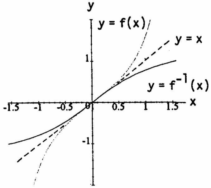
1. Yes one-to-one, the graph passes the horizontal test.
2. Not one-to-one, the graph fails the horizontal test.
3. Not one-to-one since (for example) the horizontal line y intersects the graph twice. œ#
4. Not one-to-one, the graph fails the horizontal test.
5. Domain: 1x1, Range: y
6. Domain: x, Range: y ŸŸ ŸŸ _ _ Ÿ 11 11 ## ##
7. Step 1: yx1 xy1 xy1 œ Êœ Êœ ## È
Step 2: yx1f(x) œ œ È "
8. Step 1: yx xy, since x. œÊœ Ÿ! # È
Step 2: yxf(x) œ œ È "
9. Step 1: yx1 xy1 x(y1) œ Êœ Êœ $ $ "Î$
Step 2: yx1f(x) œ œ $ " È
10. Step 1: yx2x1 y(x1) yx1, since x1 x1y œ Êœ Êœ Êœ ## ÈÈ
Step 2: y1xf(x) œ œ È "
11. Step 1: y(x1) yx1, since x1 xy1 œ Êœ Êœ # ÈÈ
Step 2: yx1f(x) œ œ È "
12. Step 1: yx xyœÊœ #Î$ $Î#
Step 2: yxf(x) œœ $Î# "
13. Step 1: yx xyœÊœ & "Î& Step 2: yxf(x); œœ & " È
98
Copyright © 2012 Pearson Education, Inc. Publishing as Addison-Wesley
Domain and Range of f: all reals; "
" "Î& " & & "Î& œœœœ
ff(x)xx and f(f(x))xxabab
14. Step 1: yx1 xy1 x(y1) œ Êœ Êœ $ $ "Î$
Step 2: yx1f(x); œ œ $ " È
Domain and Range of f: all reals; "
ff(x)(x1)1(x1)1x and f(f(x))x11xxababab ˆ‰ ab " "Î$ " $ $ $ "Î$"Î$ œ œ œœ œœ
15. Step 1: y x x œÊœÊœ""" # xyy # È
Step 2: yf(x) œœ " " È x
Domain of f: x0, Range of f: y0; " "
ff(x) x and f(f(x)) x since x0 ab " " "" "" œœœœœœ
" "" È x xx # " #x
16. Step 1: y x x œÊœÊœ""" $ xy y $ "Î$
Step 2: y f(x); œœœ "" $ " x x "Î$ É
Domain of f: x0, Range of f: y0; " " ÁÁ

ff(x) x and f(f(x)) x ab
" " "" "" "Î$ " œœœœœœ ab x xxx "Î$ $ "$
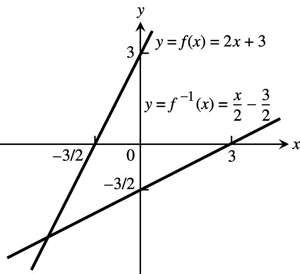
17. (a) y2x3 2xy3 œ Êœ x f(x) Êœ Êœ y 3x3 #### "
(c) 2, ¸ ¹ df df dx dx x1 x1 œ
œœ " " #
18. (a) yx7 xy7 œ Êœ"" 55 x5y35 f(x)5x35 Êœ Êœ "
(b)
(b)
œœ " "
(c) , 5 ¸ ¹ df df dx 5dx x1 xœ$%Î&
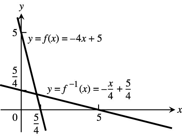
19. (a) y54x 4x5y œ Êœ x f(x) Êœ Êœ 55 x 44 44 y "
(b)
œ œ " "
(c) 4, ¸ ¹ df df dx dx 4 x1 x3 œÎ# œ
Section 2.9 Inverse Functions and Their Derivatives99
ˆ‰
Š‹ Š‹Š‹ É
ˆ‰ˆ‰
Copyright © 2012 Pearson Education, Inc. Publishing as Addison-Wesley
100 Chapter 2 Differentiation
20. (a) y2x xyœÊœ ## " # xy f(x) ʜʜ " " # È 2 x È È
œœ x ¹¹ df dx0 2 " x0 x50 œ& œ (b)
œœ "" # "Î# # È
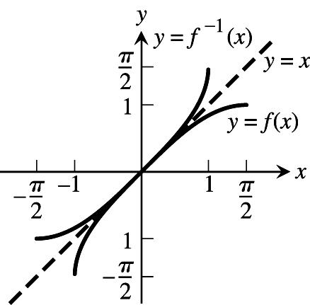
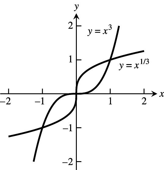
21. (a) f(g(x))xx, g(f(x))xx œœœœ ˆ‰ È È $ $ $ $
(c) f(x)3x f(1)3, f(1)3;w#ww œÊœ œ g(x)x g(1), g(1) w #Î$w w """œÊœ œ 333
(d) The line y0 is tangent to f(x)x at ();œœ!ß! $ the line x0 is tangent to g(x)x at (00)œœß $È
(b)
(c) h(x) h(2)3, h(2)3;www œÊœ œ 3x 4 # k(x)(4x) k(2), k(2) w #Î$w w "" œÊœ œ 4 333
# "
(b) 23. 3x6x 24. 2x4 df df df df dx dx 9 dx dx 6 œ Êœœ œ Êœœ
(b) The graph of yf(x) is a line through the origin with slope . œ " " m
26. ymxb x f(x)x; the graph of f(x) is a line with slope and y-intercept . œ Êœ Êœ y mmmmmm bb b " " ""
27. Let xx be two numbers in the domain of an increasing function f. Then, either xx or "# "# Á xx which implies f(x)f(x) or f(x)f(x), since f(x) is increasing. In either case, "# "#"# f(x)f(x) and f is one-to-one. Similar arguments hold if f is decreasing. "# Á
28. f(x) is increasing since xx xx; 3 #"#" """" Ê œÊœœ3636dx3dx 55dfdf " " ˆ‰ 3
œÊœÊœ
33
81x
(c) 4x20, ¸ k df dx x x5 œ& œ
22. (a) h(k(x))(4x)x, œœ " "Î$$ 4 ˆ‰ k(h(x))4x œœ Š‹ x 4 $ "Î$
" ¹¹ºº
" xf(3) xf(5) x3 x5 œ œ "" df df dx dx
(d) The line y0 is tangent to h(x) at ();œœ!ß! x 4 $ the line x0 is tangent to k(x)(4x) at œœ "Î$ () !ß!
"
25. (a) ymx xy f(x)xœÊœÊœ"" " mm
Copyright © 2012 Pearson Education, Inc. Publishing as Addison-Wesley
29. f(x) is increasing since xx 27x27x; y27x xy f(x)x; #" $$$"Î$ ""Î$ # " "" Ê
x df df dx dx81x 9 9x œÊœœœ # #Î$ """ " # #Î$ ¸ 1 3 x"Î$
30. f(x) is decreasing since xx
31. f(x) is decreasing since xx
32. f(x) is increasing since xx
33. The function g(x) is also one-to-one. The reasoning: f(x) is one-to-one means that if xx then f(x)f(x), so "#"# ÁÁ f(x)f(x) and therefore g(x)g(x). Therefore g(x) is one-to-one as well.
34. The function h(x) is also one-to-one. The reasoning: f(x) is one-to-one means that if xx then f(x)f(x), so "#"# ÁÁ , and therefore h(x)h(x). "" "# f(x)f(x) "#ÁÁ
35. The composite is one-to-one also. The reasoning: If xx then g(x)g(x) because g is one-to-one. Since "#"# ÁÁ g(x)g(x), we also have f(g(x))f(g(x)) because f is one-to-one. Thus, fg is one-to-one because "# "#ÁÁ ‰ xx f(g(x))f(g(x))."#"# ÁÊÁ
36. Yes, g must be one-to-one. If g were not one-to-one, there would exist numbers xx in the domain of g with "# Á g(x)g(x). For these numbers we would also have f(g(x))f(g(x)), contradicting the assumption that "# "#œœ fg is one-to-one. ‰
37. (gf)(x)x g(f(x))x g(f(x))f(x)1‰œÊœÊœ ww
38. The function fxx is diferentiable everywhere, and gxx is the inverse of f, so by Theorem 4 abab œœ n1/n gx x provided x0. w ab œœœœœœÁ
39-46. Example CAS commands:
Maple:
with( plots );#41
f := x -> sqrt(3*x-2);
domain := 2/3 .. 4;
x0 := 3;
Df := D(f); # (a)
plot( [f(x),Df(x)], x=domain, color=[red,blue], linestyle=[1,3], legend=["y=f(x)","y=f '(x)"],
title="#41(a) (Section 2.9)" );
q1 := solve( y=f(x), x ); # (b)
g := unapply( q1, y );
m1 := Df(x0); # (c)
t1 := f(x0)+m1*(x-x0);
y=t1;
m2 := 1/Df(x0); # (d)
t2 := g(f(x0)) + m2*(x-f(x0));
y=t2;
domaing := map(f,domain); # (e)
Section 2.9 Inverse Functions and Their Derivatives101
18x18x;
x(1y) f(x)(1x);
$$$"Î$ ""Î$ # " "" ## Ê œ Êœ Êœ 24x (1x) df df dx dx24x 6 6(x) œ Êœ œœ # #Î$ " "" " " # #Î$ ¸ 1 2 Ð Ñ1x "Î$
y18x
#"
f(x)1x;
""Î$ Ê œ Êœ Êœ 3(1x) x df df dx dx3(1x) 3 3x œ Êœ œœ # #Î$ " "" " # #Î$ ¹ 1x"Î$
(1x)(1x); y(1x) x1y
#"#"$$$"Î$
xy f(x)x;
&Î$&Î$ # " &Î$ $Î& "$Î& Ê œÊœÊœ x x df5 df 33 dx3 dx 5 x 5x œÊœœœ #Î$ #Î&
xx; yx
#"
" " #Î$ #Î& ¹ 5 3 x$Î&
Á Á
"# "#
n gx n x n x n x 1/n1 w ab ab ab ab ab ab n1 n1 1/n n1/n 11/n ab
111111 fgxn
Copyright © 2012 Pearson Education, Inc. Publishing as Addison-Wesley
Chapter 2 Differentiation
p1 := plot( [f(x),x], x=domain, color=[pink,green], linestyle=[1,9], thickness=[3,0] ):
p2 := plot( g(x), x=domaing, color=cyan, linestyle=3, thickness=4 ):
p3 := plot( t1, x=x0-1..x0+1, color=red, linestyle=4, thickness=0 ):
p4 := plot( t2, x=f(x0)-1..f(x0)+1, color=blue, linestyle=7, thickness=1 ):
p5 := plot( [ [x0,f(x0)], [f(x0),x0] ], color=green ):
Mathematica:
display( [p1,p2,p3,p4,p5], scaling=constrained, title="#41(e) (Section 2.9)" ); (assigned function and values for a, b, and x0 may vary)
If a function requires the odd root of a negative number, begin by loading the RealOnly package that allows Mathematica to do this.
<<Miscellaneous `RealOnly`
Clear[x, y]
{a,b} = {2, 1}; x0 = 1/2 ;
f[x_] = (3x2) / (2x11)
Plot[{f[x], f'[x]}, {x, a, b}]
solx = Solve[y == f[x], x]
g[y_] = x /. solx[[1]]
y0 = f[x0]
ftan[x_] = y0f'[x0] (x-x0)
gtan[y_] = x01/ f'[x0] (yy0)
Plot[{f[x], ftan[x], g[x], gtan[x], Identity[x]},{x, a, b}, EpilogLine[{{x0, y0},{y0, x0}}], PlotRange{{a,b},{a,b}}, AspectRatioAutomatic]ÄÄÄ 47-48. Example CAS commands:
Maple:
with( plots );
eq := cos(y) = x^(1/5);
domain := 0 .. 1;
x0 := 1/2;
f := unapply( solve( eq, y ), x ); # (a)
Df := D(f);
plot( [f(x),Df(x)], x=domain, color=[red,blue], linestyle=[1,3], legend=["y=f(x)","y=f '(x)"],
title="#48(a) (Section 2.9)" );
q1 := solve( eq, x ); # (b)
g := unapply( q1, y );
m1 := Df(x0); # (c)
t1 := f(x0)+m1*(x-x0);
y=t1;
m2 := 1/Df(x0); # (d)
t2 := g(f(x0)) + m2*(x-f(x0));
y=t2;
domaing := map(f,domain); # (e)
p1 := plot( [f(x),x], x=domain, color=[pink,green], linestyle=[1,9], thickness=[3,0] ):
p2 := plot( g(x), x=domaing, color=cyan, linestyle=3, thickness=4 ):
p3 := plot( t1, x=x0-1..x0+1, color=red, linestyle=4, thickness=0 ):
p4 := plot( t2, x=f(x0)-1..f(x0)+1, color=blue, linestyle=7, thickness=1 ):
p5 := plot( [ [x0,f(x0)], [f(x0),x0] ], color=green ):
Mathematica:
display( [p1,p2,p3,p4,p5], scaling=constrained, title="#48(e) (Section 2.9)" ); (assigned function and values for a, b, and x0 may vary)
For problems 47 and 48, the code is just slightly altered. At times, different "parts" of solutions need to be used, as in the definitions of f[x] and g[y]
102
Copyright © 2012 Pearson Education, Inc. Publishing as Addison-Wesley
2.10
Clear[x, y]
{a,b} = {0, 1}; x0 = 1/2 ; eqn = Cos[y] == x1/5
soly = Solve[eqn, y]
f[x_] = y /. soly[[2]]
Plot[{f[x], f'[x]}, {x, a, b}] solx = Solve[eqn, x]
g[y_] = x /. solx[[1]]
y0 = f[x0]
ftan[x_] = y0f'[x0] (xx0)
gtan[y_] = x01/ f'[x0] (yy0)
Plot[{f[x], ftan[x], g[x], gtan[x], Identity[x]},{x, a, b}, EpilogLine[{{x0, y0},{y0, x0}}], PlotRange{{a, b}, {a, b}}, AspectRatioAutomatic]
FUNCTIONS
Section 2.10 Logarithmic Functions103
ÄÄÄ
LOGARITHMIC
1. (a) ln 0.75ln ln 3ln 4ln 3ln 2ln 32 ln 2 œœ œ œ 3 4 # (b) ln ln 4ln 9ln 2ln 32 ln 22 ln 3 4 9 œ œ œ ## (c) ln ln 1ln 2ln 2 (d) ln 9 ln 9 ln 3 ln 3 " "" # $ # œ œ œœœ È 333 2 (e) ln 32ln 3ln 2ln 3 ln 2 È œ œ "Î# " # (f) ln 13.5 ln 13.5 ln ln 3ln 2(3 ln 3ln 2) È ab œœœ œ """" ##### $ 27 2. (a) ln ln 13 ln 53 ln 5 (b) ln 9.8ln ln 7ln 52 ln 7ln 5 " # 125 5 49 œ œ œœ œ (c) ln 77ln 7 ln 7 (d) ln 1225ln 352 ln 352 ln 52 ln 7 È œœ œœœ $Î# # # 3 (e) ln 0.056ln ln 7ln 5ln 73 ln 5 œœ œ 7 125 $ (f) ln 35 ln ln 25 ln 5 ln 5 ln 7 ln 7 " ## " 7 œœ 3. (a) ln sin lnln ln 5 (b) ln3x9xlnln ln(x3) ) œœ œœ ˆ‰ ˆ‰ ab Š‹ sin sin 3x 9x 5 3x 3x )) Š‹ sin 5 ) # " # (c) ln4tln 2ln 4tln 2ln 2tln 2lnlnt " # # %## % ab ab È Š‹ œ œ œœ 2t# 4. (a) ln sec ln cos ln[(sec )(cos )]ln 10 ))))œœœ (b) ln(8x4)ln 2ln(8x4)ln 4lnln(2x1) œ œœ # ˆ‰ 8x 4 4 (c) 3 ln t1ln(t1)3 lnt1ln(t1)3 lnt1ln(t1)ln È abab ˆ‰ Š‹ 3 # ## "Î$ " " œ œ œ 3(t 1) (t 1)(t ) ln(t1) œ 5. (a) e7.2 (b) e (c) ee ln7.2 lnx lnxlnylnxy e xy x œœ œœ œ ÐÎÑ "" # # # lnx 6. (a) exy (b) e (c) ee lnxy ln03 lnxln2lnx2 e 0.3 x ab ## ## Þ ÐÎÑ "" # œ œœ œœ ln03 11 1 7. (a) 2 ln e2 ln e(2) ln e1 (b) lnln eln(e ln e)ln e1 È ˆ‰ ab œœœ œœœ "Î# " # e (c) lne xy ln exy ab #### xy## œ œ ab Copyright © 2012 Pearson Education, Inc. Publishing as Addison-Wesley
104 Chapter 2 Differentiation
8. (a) lne(sec )(ln e)sec (b) ln ee(ln e)e ˆ‰ ab sec ex x ) œœ œœ )) ab x
(c) lnelneln x2 ln x ˆ‰ Š‹ 2lnx lnx œœœ # #
9. ln y2t4 ee ye 10. ln yt5 ee ye œ ʜʜœ ʜʜ lny2t4 2t4 lnyt5 t5
11. ln(y40)5t ee y40e ye40 œÊœÊ œÊœ lny40)5t 5t 5t Ð
12. ln(12y)t ee 12ye 2ye1 y œÊœÊ œÊ œ Êœ ln12y)t t t e Ð " # Š‹ t
13. ln(y1)ln 2xln x ln(y1)ln 2ln xx lnx ee e œ Ê œÊœÊœÊœ ˆ‰ y1 y1 2x x ln x x # ˆ‰ y1 2x y12xe y2xe1 Ê œÊœxx
14. lny1ln(y1)ln(sin x) lnln(sin x) ln(y1)ln(sin x) ee ab Š‹ # Ð ÑÐÑ " œÊœÊ œÊœ y y1 lny1lnsinx # y1sin x ysin x1 Ê œÊœ
15. (a) e4 ln eln 4 2k ln eln 2 2k2 ln 2 kln 2 2k 2k œÊœÊœÊœÊœ #
(b) 100e200 e2 ln eln 2 10k ln eln 2 10kln 2 k 10k 10k 10k ln 2 10 œÊœÊœÊœÊœÊœ
(c) ea ln eln a ln eln a ln a k1000 ln a k1000 k1000 kk 1000 1000 ÎΜʜʜʜʜ
16. (a) e ln eln 4 5k ln eln 4 5kln 4 k 5k 5k 4 5 ln 4 œÊœÊœ Êœ Êœ " "
(b) 80e1 e80 ln eln 80 k ln eln 80 kln 80 kkk œÊœÊœÊœ Êœ " "
(c) e0.8 e0.8 (0.8)0.8 k1 ÐÞÑln08k ln08 k k œÊœÊœÊœ
ˆ‰
17. (a) e27 ln eln 3 (0.3t) ln e3 ln 3 0.3t3 ln 3 t10 ln 3 Þ Þ$ 03t 03t œÊœÊ œÊ œÊœ
(b) e ln eln 2kt ln eln 2 t kt kt ln 2 k œÊœœœ Êœ " # "
(c) e0.4 e0.4 0.20.4 ln 0.2ln 0.4 t ln 0.2ln 0.4 t ÐÞÑ ln02t ln02 t t t ln 0.4 ln 0.2 œÊœÊœÊœÊœÊœ
ˆ‰
18. (a) e1000 ln eln 1000 (0.01t) ln eln 1000 0.01tln 1000 t100 ln 1000 Þ Þ 001t 001t œÊœÊ œÊ œÊœ
(b) e ln eln 10kt ln eln 10 ktln 10 t kt kt 10 k ln 10 œÊœœœ Êœ Êœ " "
(c) e e2 22 t1 ÐÑ " " " # ln2t ln2 t t œÊœÊœÊœ
ˆ‰
ÈÈ
È 20.
œÊœÊœÊœ 21. (a) 57 (b) 82 (c) 1.375 log7 log2 log75 5 8 13 œœœ È È
(e) log 3log 3 log 310.5 444 333 œœœœ œœœœœ # "Î# """ ### È
log
444 ˆ‰
4 œœ œ œ 22. (a) 23 (b) 10 (c) 7 log3 log12 log7 2 10 œœœ ÐÎÑ " # 1 1
œœœœ
œœœœ
ˆ‰ˆ‰
333 ˆ‰
9 œœ œ œ Copyright © 2012 Pearson Education, Inc. Publishing as Addison-Wesley
19. ex ln eln x t2 ln x t4(ln x)
tt œÊœÊœÊœ ## #
eee ee ln eln e tx2x1 x2x1tx2x1tx2x1t ### #
(d) log 16log 42 log 4212
(f)
log 41 log 4111
" "
(d) log 121log 112 log 11212 11 11 11
# (e) log 11log 121 log 1211 121 121 121
"Î# """ ###
(f) log log 32 log 3212
" #
23. (a) Let zlog x 4x 2x 2x 2xœÊœÊœÊœÊœ 4 z2zzz ab È #
(b) Let zlog x 3x 3x 3x 9xœÊœÊœÊœÊœ 3 zz2zz ab# ###
(c) log elog 2sin x 22 ln2 sinxsinxab ÐÑ œœ
24.
Let zlog 3x 53x 259xœÊœÊœ 5 zz ab##%
(b) log ex e x ab œ
aln aln bln
yln kx y(k) œÊœœ œÊœœ w w """ ˆ‰ ˆ‰ 1 3xxkxx 29. ylnt (2t)
31.
" 32.
yln ln 10x 10x œœÊœ œ 10 xdx10xx dy " # ""
yln x 3x
(c) t 42. y œÊœœœ " " ln t 1ln tln t tdt tt dy t(ln t)(1) t ˆ‰ " #
ylnt t œÊœœ œÊœœ ab ˆ‰
log a log aln xln xln xln t " ## 43. y y œÊœœœ ln x 1ln xx(1ln x) (1ln x)(ln x) (1ln x) (1ln x) w " ˆ‰ˆ‰ """ xxxxx ln xln x ## # 44. y y 1 œÊœ œœ x ln x ln x 1ln x(1ln x)(1ln x) (1ln x) (x ln x) (1ln x) (ln x)ln x w " ˆ‰ˆ‰ ln xx "" xx #
"" "" #
34.
y(ln x) 3(ln x)(ln x) œÊœœ œÊœœ $# $# " dy dy 3(ln x) dxx x dx dx x 3 d
yt(ln t) (ln t)2t(ln t)(ln t)(ln t)(ln t)2 ln t œÊœ œ œ ## ## dy dt dt t d 2t ln t † 38. ytln tt(ln t) (ln t)t(ln t)(ln t)(ln t) (ln t) œœÊœ œ œ È "Î# "Î# "Î# "Î# "Î# " " ## # dy t(ln t) dt dt t d (ln t) † "Î#
aln aln aln x2 ln x x x# # # œƒœœœ # ## Copyright © 2012 Pearson Education, Inc. Publishing as Addison-Wesley
#
Logarithmic
Section 2.10
Functions105
(a)
25. (a) (b) log x log x log xln ln 3ln ln xln 2 log xln ln 8ln ln xln ln xln xln xln 3ln 3 ln xln xln xln 83 ln 2 2 2 3 8 œƒœœ œƒœœ ## ## 2 œ 3
2
aln x ln
26. (a) log x log xln 9ln 32 ln 3ln x2 ln xln xln xln 31 9 3 œƒœœ (b) log x log xln xln 10 ln xln xln xln 2 ln 10 ln 2 ln 10 ln 2 È È 10 2 œƒœœ ÈÈ ˆ‰ ˆ‰ " # " # (c) log b log
ˆ‰ˆ‰ˆ‰
ˆ‰ab
ˆ‰ab " 33.
ˆ‰ ˆ‰
35.
ˆ‰ab
(c) log 2log 4 44 eeˆ‰xx x sinx sinx e sin x œœ ˆ‰Î# # "Î# 39. y ln x x ln x x ln x œ Êœ œ xx x4x 416dx4x16 dy %% %$ $$ " † 40. y ln x x ln x x ln x œ Êœ œ xx x3x 39dx3x9 dy $$ $# ## " 41. y œÊœœ ln t tdt dy t(ln t)(1) tt 1ln t ˆ‰ " ##
aln aln a ln bln aln bln bln b a b œƒœœ ˆ‰#
27.
yln 3x y(3)
28.
30.
# $Î#"Î# " " # dy dy dtt t dt 2t 2 33 t # $Î#
yln ln 3x 3x œœÊœ œ 3 xdx3xx dy " # ""
yln(1) (1)
yln(22) (2) œ Êœœ œ Êœœ )) dy dy d 1 1d 2 1 ))))))
36.
$
37.
106 Chapter 2 Differentiation
45. yln(ln x) y œÊœœ w """
ln xxx ln x
46. yln(ln(ln x)) y (ln(ln x)) (ln x) œÊœœœ w """" ln(ln x)dxln(ln x)ln xdxx(ln x) ln(ln x) dd
47. y[sin(ln )cos(ln )] [sin(ln )cos(ln )]cos(ln )sin(ln ) œ Êœ )))))))) dy d ))) ‘ "" sin(ln )cos(ln )cos(ln )sin(ln )2 cos(ln ) œ œ )))))
48. yln(sec tan ) sec œ Êœœœ )) ) dy sec (tan sec ) dsec tan tan sec sec tan sec ))))) ))) ))) #
49. yln ln x ln(x1) y œœ Êœ œ œ """ " " ## w xx1 xx12x(x1)2x(x1) 2(x1)x 3x2
50. y ln ln(1x)ln(1x) y (1) œœ Êœ œœ " " """ " " # # # # " w 1x 1x1x 1x 1x1x (1x)(x)1x cd ‘
51. y œÊœœœ 1ln t 2 1ln tdt(1ln t)(1ln t)t(1ln t) dy (1ln t)(1ln t) ˆ‰ˆ‰ " """ t ttttt ln tln t ## #
52. yln tln t ln t ln tln t t œœÊœ œ
"Î# "Î# "Î# "Î# "Î# "Î# "Î# "Î# "" " ## dy dt dt dt dd t"Î# ln t t œœ "" "" ## "Î# "Î# "Î# ˆ‰ t 4tln t "Î#
53. yln(sec(ln )) (sec(ln )) (ln ) œÊœœœ ))) dy sec(ln ) tan(ln ) tan(ln ) dsec(ln )d sec(ln )d dd ))) ))) )) ) "
54. yln (ln sin ln cos )ln(12 ln ) œœ Êœ È sin cos 12 ln dsin cos 1 ln dy cos sin )) )) ) ) ) )) # # # "" ))) ˆ‰ 2 ) cot tan œ " # ’“ )) 4 (12 ln ) ))
#
5205 ## ## "" w & #! œ 53x2 (x1)(x) # # ’“
57. yx(x1)(x(x1)) ln y ln(x(x1)) 2 ln yln(x)ln(x1) œ œ Êœ Êœ Êœ È "Î# " "" # 2y yxx1 w yx(x1)Êœ œœ w """ " # ˆ‰ˆ‰ È xx12x(x1) x(x1)(2x1) 2x 2x(x1) È È 58. yx1(x1) ln ylnx12 ln(x1) œ Êœ Êœ Èabcd ab ˆ‰ ## "" ## # y yx1x1 2x2 w # yx+1(x1) x1(x1) Êœ œ œ w #### " ÈÈ abab ˆ‰ ’“
ˆ‰ˆ‰
È ˆ‰
ˆ‰ ’“
É
È ˆ‰ˆ‰ˆ‰ˆ‰ˆ‰
É È
55. yln
lnx1 ln(1x)
(1) œœ Êœ œ Š‹ ab ˆ‰ ab È x1 1x 52x 10x x11xx1(1x) # & ## #w"" "" # # # 56. yln [5 ln(x1)20 ln(x2)] y œœ Êœ œ É ˆ‰ ’“ (x1) (x2)4(x1) (x2)x1x(x1)(x2)
5
y
xx x x 1 x1x1 x1(x1) 2xx1 x1 x1(x1)
# # ab abkk È 59. y ln y[ln tln(t1)] œœÊœ Êœ É ˆ‰ ˆ‰ tt t1t1ydttt1 dy ## "Î# """"" Êœ œœ dy dtt1tt1t1t(t1) tt 2t(t1) """""" # # ÉÉ ˆ‰ ’“ È $Î# 60. y [t(t1)] ln y[ln tln(t1)] œœ Êœ Êœ É ˆ‰ 1 t(t1)ydttt1 dy ## "Î# """"" Êœ œ dy dtt(t1)t(t1) 12t2t1 2tt " " # É ’“ ab # $Î# Copyright © 2012 Pearson Education, Inc. Publishing as Addison-Wesley
## ##
61. y3(sin )(3) sin ln y ln(3)ln(sin ) œ œ Êœ Êœ È )))))) "Î# """ ##yd(3)sin dy cos ))) ) 3(sin )cot Êœ dy d2(3) )) È ’“ ))) "
62. y(tan )21(tan )(21) ln yln(tan ) ln(21) œ œ Êœ Êœ )))))) È ˆ‰ˆ‰ "Î# """ ### ydtan 1 dy sec2 ))) ) # (tan )21 sec21 Êœ œ dy dtan 1 sectan 21 ))) )) ) )) ))ÈÈ Š‹ ab # " # # È
63. yt(t1)(t2) ln yln tln(t1)ln(t2) œ Êœ Êœ"""" # ydttt1t dy t(t1)(t+2) t(t1)(t2) 3t6t2 Êœ œ œ dy (t1)(t2)t(t2)t(t1) dt tt1t t(t1)(t2)
""" # #
64. y ln yln 1ln tln(t1)ln(t2) œÊœ Êœ " """" # t(t1)(t2)ydttt1t dy Êœ œ dy (t1)(t2)t(t2)t(t1) dtt(t1)(t2)tt1tt(t1)(t) t(t1)(t2) """" " # # ‘
œ 3t6t2 t3t2t # $# #ab
65. y ln yln(5)ln ln(cos ) œÊœ Êœ ) ) )))))) """ 5 sin cos yd5cos dy ))) tan Êœ dy d cos 5 5 ))))) ) ˆ‰ˆ‰ "" )
66. y ln yln ln(sin ) ln(sec ) œÊœ Êœ )) ) ) )))) )) sin cos sec ydsin 2 sec dy(sec )(tan ) È )))""" # ’“ cot tan Êœ dy d sin sec )) )) ) È ˆ‰ "" # ))
"" # # ab y Êœ w " xx1 (x1) xx13(x1) x2 È # #Î$ # ’“
w #
67. y ln yln x lnx1 ln(x1) œÊœ Êœ xx1 y (x1) 2x 2 3 yxx13(x1) È # #Î$
68. y ln y[10 ln(x1)5 ln(2x1)] œÊœ Êœ É (x1) y (2x1) yx12x1 55 # " "! &
w y Êœ w É ˆ‰ (x1) (2x1)x12x1 55 "! &
69. y ln yln xln(x2)lnx1 œÊœ Êœ É cd ab ˆ‰ 3 x(x2) y x1 3 y3xxx1 2x # "" " " # # #
w y Êœ w """ # 3x1xxx1 x(x2) 2x É ˆ‰ 3 ##
70. y ln yln xln(x1)ln(x2)lnx1ln(2x3) œ Êœ É cd ab 3 x(x1)(x2) x1(2x3)3 " # ab # y Êœ w """" # 3x1(2x3)xx1xx12x3 x(x1)(x2) 2x2 É ˆ‰ 3 ab##
71. ylncos 2cossin2tanœÊœ†† œ ab ab 2 dy dcos 1 )) )) )) 2
72. yln3eln 3ln ln eln 3ln 1 œœ œ Êœ ˆ‰)))) " )) )) dy d 73. yln3teln 3ln tln eln 3ln tt 1 œœ œ Êœ œ ab " tt dy dttt 1t 74. yln2e sin tln 2ln eln sin tln 2tln sin t 1 (sin t)1 œœ œ Êœ œ ab
Section 2.10 Logarithmic Functions107
ˆ‰ ’“
’“
Copyright © 2012 Pearson Education, Inc. Publishing as Addison-Wesley
ˆ‰ " tt dy dtsin tdtsin t dcos t œ cos tsin t sin t
108 Chapter 2 Differentiation
75. yln ln eln1eln1+e 1 1e1 œœ œ Êœ œ œ e de 1e 1e1e1e dy dd ) ) ) )) )
"")))) )) ˆ‰ˆ‰ˆ‰ˆ‰ )
76. yln ln ln1 1 œœ Êœ È ÈÈÈ ) )))))) 1 1 dy dd d dd"" ÈÈÈÈ
Š‹Š‹Š‹Š‹Š‹ ))))
œ œœœ Š‹Š‹Š‹Š‹ """" "" # # # # ÈÈÈÈ Š‹ÈÈ
ÈÈ ab )))) )) )))) )) 1 1 21 1 1 "Î#
Š‹Š‹
77. yeeete ete (cos t)(1t sin t)e œœœÊœ œ Ð Ñ costln tcostlntcostcostcostcost dy dtdt d
78. yeln t1 e(cos t)ln t1eeln t1(cos t) œ Êœ œ sint sint sintsint dy dt t t 22 ab abab ‘ ###
79. ln ye sin x yye(sin x)e cos x ye sin xe cos x œÊœ Ê œ yy yy y yyŠ‹
ab "" www y e cos x y ÊœÊ œ ww Š‹ 1ye sin x ye cos x y 1ye sin x y yy y
80. ln xye ln xln ye y1ye yee œÊ œÊ œ Ê œ xy xy xy xyxy xy y x w w w "" " "
y y ʜʜ ww " "
1ye yxx1ye xe yxe xy xy xy xy ab ab
2 2
82. tan yeln x secyye y œ Êœ Êœ xx xx xe cosy ab#w w " " ab x #
Š‹
Š‹
Š‹
Š‹
ab
Š‹
83. y2 y2 ln 2 84.
œÊœ œÊœ
xx
81. xylnxlnyylnxxlnyyylnxxy1lnylnxyylny yxyx 11x xyyx y œÊœÊœÊ† †œ†† †Ê† †œ www w ab y Êœœœ w lny lnxxylnxxxylnxx xylnyyyxlnyy y x x y w w 85. y5 5(ln 5)s 5 œÊœ œ ÈÈ È ss s dy ds ln 5 2s ˆ‰ Š‹ " # "Î# È 86. y2 2(ln 2)2sln 2s2(ln 4)s2 œÊœœœ ss ss dy ds ## ##abŠ‹ # 87. yx yx 88. yt (1e)t œÊœ œÊœ 11 w 1 Ð Ñ 11 e e dy dt 89. ylog 5 (5) œœÊœœ 2 ) ln 5 ln dln 5 ln dy ) ))) ### """ˆ‰ˆ‰ 90. ylog (1 ln 3) (ln 3) œ œÊœ œ 3 ) ln(1 ln 3)dy ln 3dln 31 ln 31 ln 3 """ ) ))) ˆ‰ˆ‰ 91. ylogxlogx 2 3 y œ œ œ œÊœ 44 2 ln xln xln xln xln x3 ln 4ln 4ln 4ln 4ln 4x ln 4 # w 92. ylogelogx (xln x) y1 œ œ œ œ Êœ œ 25 5 x x ln eln xxln x x1 ln 52 ln 5 ln 52 ln 5 ln 5 ln 5x2x ln 5 È ˆ‰ˆ‰ˆ‰### # "" " w 93. ylog rlog r (2 ln r) œœœÊœœ 24 ˆ‰ˆ‰ˆ‰ ’“ ln rln rlnr 2 ln r ln ln 4(ln 2)(ln 4)dr(ln 2)(ln 4) rr(ln 2)(ln 4) dy # "" # 94. ylog rlog r (2 ln r) œœœÊœœ 39 ˆ‰ˆ‰ˆ‰ ’“ ln rln rlnr 2 ln r ln 3ln 9(ln 3)(ln 9)dr(ln 3)(ln 9) rr(ln 3)(ln 9) dy # "" Copyright © 2012 Pearson Education, Inc. Publishing as Addison-Wesley
y3 y3(ln 3)(1)3 ln 3
œ
xxx
))
œ dy d(sin )(ln 7)(cos )(ln 7)ln 7ln 7ln 7 cos sin ln 2 ))) ))
))
tan 1ln 2)
100.
xe 2x1 ln xln eln 2ln x1 ln 2ln
È
2 2 ln x2ln 2 ln(x1)
ˆ‰ˆ‰ ’“"" " ##
œœœÊœœÊœ œ ˆ‰ˆ‰ˆ‰ˆ‰ˆ‰ˆ‰ È t t tt "Î# Î# ### # # """" Î# tt ln t ydt t dy t Êœ dy dt ln t
t ## "
ˆ‰
" yxÊœ w sinx ’“ sin xx(ln x)(cos x) x
ˆ‰
cd w
Section 2.10 Logarithmic Functions109 95. ylog lnln(x1)ln(x1)œœœœœ 3 ln3 Š‹ˆ‰ˆ‰ x1 x1 x1 ln 3 ln 3 x1 (ln 3) ln ln ˆ‰ x1 x1 ln3 x1 x1 Š‹ Êœ œ dy dxx1x1(x1)(x1) 2 "" 96. ylog log ln œœœœœ 55 ln5ln52 Ɉ‰ˆ‰ˆ‰ˆ‰ ”• 7x 7x ln 5 7x 3x2 3x2 ln 5 ln 5 3x ## # " ÐÑÎ ln ln ˆ‰ ˆ‰ 7x 7x 3x2 3x2 ln52ÐÑÎ ln 7x ln(3x2) œ Êœ œœ "" " ## dy(3x2)3x dx27x2(3x2)2x(3x2)x(3x2) 73 97. y sin(log ) sin sincos sin(log ) cos(log ) œœÊœ œ ))) ) )) 7 77 ˆ‰ˆ‰ ˆ‰‘ˆ‰ ln
"" 98.
(cot
ʜ
ln ln ln 7dln 7ln 7 ln 7ln 7 dy ))) )) ""ˆ‰
ylogœœœ 7 ˆ‰ sin cos e ln(sin )ln(cos )ln eln 2ln(sin )ln(cos ) ln 2 ln 7ln 7 )) )))))) ) #)
Š‹
È
2)2x(x1)ln 4(x1)x 101. y33 3(ln 3) log 33 œœÊœ œ logtlntln2 lntln2 logt 2 2 2 ÐÑÎÐÑ ÐÑÎÐÑ dy dtt ln 2t cdab ˆ‰"" 102. y3 log (log t) œœœÊœœœ 82 3 ln(log t) dy ln 8ln 8dtln 8(ln t)/(ln 2)t ln t(ln t)(ln 8)t(ln t)(ln ) 3 ln 33 2 ln t ln 2 ˆ‰
103. ylog 8t 3ln t œœœœ Êœ 2 ln2 ab ln 8lnt ln ln dtt 3 ln 2(ln 2)(ln t)dy ## " ˆ‰ ln2 104. ytloge t sin t sin tt cos t œœœœœÊ œ 3 sintln3 t lne ln 3ln 3ln 3dt t ln3 t(sin t)(ln 3)dy ˆ‰ abab Š‹ ˆ‰ ˆ‰ ln3 sint sint 105. y(x1) ln yln(x1)x ln(x1) ln(x1)x y(x1)ln(x1) œ Êœ œ Êœ Êœ xx x y y(x1)x1 x w " w ‘ 106. yx ln yln x(x1) ln x ln x(x1)ln x1 yx1ln x œÊœœ Êœ œ Êœ Ð "Ñ Ð "Ñ Ð Ñ xx x1 y yxxx w ˆ‰ ˆ‰""" w 107. yttt ln yln t ln t (ln t)
ˆ‰ˆ‰ È
108.
99. ylog e y œœœÊœ 5 x ln ex ln 5ln 5ln 5 x w "
ylogœœœ 2
## ## " #
y Êœ œœ w " # # 23x4 x ln 2(ln 2)(x1)2x(x1)(ln
ytt ln yln tt(ln t) t(ln t)t œœÊœœÊœ œ È ˆ‰ˆ‰tt t "Î# "Î# ˆ‰ ˆ‰ˆ‰ "Î# "Î# "Î# "" " # ydt t dy ln t2 2t È t Êœ dy dt ln t2 2t Š‹ È È t
109. y(sin x) ln yln(sin x)x ln(sin x) ln(sin x)x y(sin x)ln(sin x)x cot x œÊœœÊœ Êœ xx x y ysin x cos x w
Copyright © 2012 Pearson Education, Inc. Publishing as Addison-Wesley
110. yx ln yln x(sin x)(ln x) (cos x)(ln x)(sin x) œÊœœÊœ œ sinx sinx y sin xx(ln x)(cos x) yx x w
113. (a) Begin with yln x and reduce the y-value by 3yln x3. œÊœ
(b) Begin with yln x and replace x with x1ylnx1. œ Êœ ab
(c) Begin with yln x, replace x with x1, and increase the y-value by 3ylnx13. œ Êœ ab
(d) Begin with yln x, reduce the y-value by 4, and replace x with x2ylnx24. œ Êœ ab
(e) Begin with yln x and replace x with xylnx. œ Êœ ab
(f) Begin with yln x and switch x and yxln y or ye.œÊœœ x
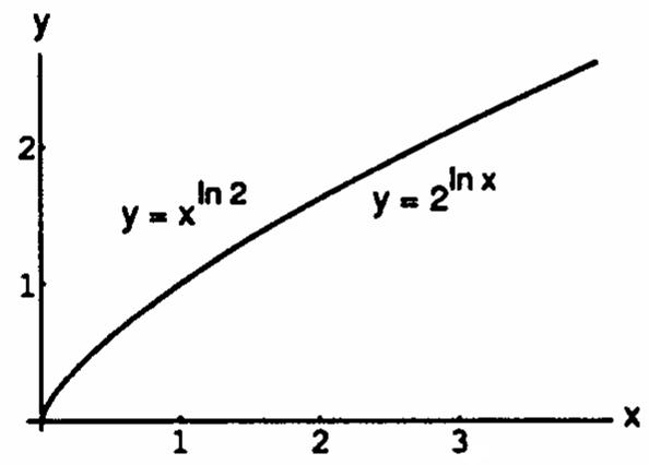
114. The functions f(x)x and g(x)2 appear to œœ ln2 lnx have identical graphs for x0. This is no accident, because xee2. ln2ln2lnxln2 lnx lnx œœœ ab
115. yAsinlnxBcoslnxyAcoslnxBsinlnxAcoslnxBsinlnx œ Êœ† †œ † ababababab abab w 111 xxx yAcoslnxBsinlnx AsinlnxBcoslnx
† † †† ww a ababbababˆ‰ 111 1 xxx x 2 AcoslnxsinlnxBsinlnxcoslnx œ † ab abab abababab 1 x2 xyxyyAcoslnxsinlnxBsinlnxcoslnxAcoslnxBsinlnx
a b a ba ababababbabab AsinlnxBcoslnx
110 Chapter
111. yx, x0 ln y(ln x) 2(ln x) yx œ ʜʜʜ lnx lnx #w " y yxx ln x w # ˆ‰ abŠ‹ 112. y(ln x) ln y(ln x)ln(ln x) ln(ln x)(ln x) (ln x) œÊœÊœ œ lnx yln (ln x) yx ln xdxxx d w ˆ‰ ˆ‰ """ y (ln x) Êœ w " Š‹ ln(ln x) x lnx
2 Differentiation
ʜ
116. lim 1 lim e for any x0. 1 nn Ä_Ä_ ˆ‰ ”• Š‹ œœ x n n 1 n/x n/x x x ab ab 117. (a) Amount8 œ ˆ‰ 1 2 t12 Î (b) 81 3t36 ˆ‰ˆ‰ˆ‰ˆ‰ 111 11t 228 2212 t12 t12 t123ÎÎÎ œÄœÄœÄœÄœ There will be 1 gram remaining after 36 hours. 118. yye represents the decay equation; solving 0.9yyet0.585 days œœÊœ¸ 00 0 0.18t 0.18t ln0.9 0.18 ab ab 2.11 INVERSE TRIGONOMETRIC FUNCTIONS 1. (a) (b) (c) 2. (a) (b) (c) 111 111 436 436 3. (a) (b) (c) 4. (a) (b) (c) 111 111 643 643 5. (a) (b) (c) 6. (a) (b) (c) 111 111 346 346 32 5 7. (a) (b) (c) 8. (a) (b) (c) 32 5 463 463 111 111 9. (a) (b) (c) 10. (a) (b) (c) 111 111 436 436 Copyright © 2012 Pearson Education, Inc. Publishing as Addison-Wesley
Ê œ 2 www ab
œ! ab abab
11. (a) (b) (c) 12. (a) (b) (c) 32 5 463 463 111 111 13. lim sinx 14. lim cosx x1 x1ÄÄ " " # œœ 1 1 15. lim tanx 16. lim tanx xx Ä_Ä_ " " # # œœ 1 1 17. lim secx 18. lim secx lim cos xx x Ä_Ä_Ä_ " " " # # " œœ œ 1 1 ˆ‰ x 19. lim cscx lim sin0 20. lim cscx lim sin0 xx xx Ä_Ä_Ä_Ä_ " " " " " " œœ œœ ˆ‰ ˆ‰ x x 21. ycosx 22. ycossec x œÊœ œœœÊœ "# " " "" ab ˆ‰ dy dy dxxdx 2x2x 1x 1x x x1 É ab È È kk # # % # 23. ysin2t 24. ysin(1t)œÊœœœ Êœœ " " " " È dy 2 2 dy dt dt 12t 12t 2tt 1(1t) ÈÈ ÊŠ‹ È ÈÈ È # # # # 25. ysec(2s1) œ Êœœœ " " dy ds 22 2s1 (2s1)1 2s1 4s4s2s1 ss kk ÈÈÈ kkkk # ## 26. ysec5sœÊœœ " " dy ds 5 5s (5s)1 s 25s1 kk ÈÈ kk # # 27. ycscx1 œ Êœ œ "#ab dy dx 2x2x x1 x11 x1 x2x kkab É ab È ## # # %# 28. ycscœÊœ œœ " # " ˆ‰x2 dy dx 1 x x x4 Š‹ ÉÉ ˆ‰ kk kk È " # ## # ¸¸xx x4 4 # # 29. yseccost œœÊœ " " " " ˆ‰tdt dy 1t È # 30. ysincsc œœÊœ œœ " " ˆ‰ Š‹3t 2t6 t3dt dy 1 t tt9 # # # # % ˆ‰ ¹¹Š‹ 2t 3 tt 33 t9 9 ## % Ê É È 31. ycottcott œœÊœ œ " ""Î# " # È dy dt t 1t t(1t) Š‹ ab È " # "Î# "Î# # 32. ycott1cot(t1) œ œ Êœ œœ " ""Î# " " È dy dt (t1) 1(t1) 2t1(1t1)2tt1 Š‹ cd ÈÈ " # "Î# "Î# # 33. ylntanxœÊœœ ab " " dy dxtanxtanx1x Š‹ abab " # 1x " "# 34. ytan(ln x) œÊœœ " " dy dx1(ln x)x1(ln x) ˆ‰ " x ## cd 35. ycsceœÊœ œ " " ab t dy dt e e e1 e1 t tt 2t kkab É È # 36. ycoseœÊœ œ " ab t dy dt ee 1e 1e # tt t 2t É ab È Copyright © 2012 Pearson Education, Inc. Publishing as Addison-Wesley University Calculus Elements with Early Transcendentals 1st Edition Hass Solutions Manual Full Download: http://testbanktip.com/download/university-calculus-elements-with-early-transcendentals-1st-edition-hass-solutions-manual/ Download all pages and all chapters at: TestBankTip.com
Section 2.11 Inverse Trigonometric Functions111
