Chapter 2 Investment Decisions: The Certainty Case
Using
Alternatively, equation
can be used:
Sales cash inflows $140,000 Operating costs = cash outflows 100,000 Earnings before depreciation, interest and taxes 40,000 Depreciation (Dep) 10,000 EBIT 30,000 Taxes @ 40% 12,000 Net income $18,000
equation 2-13: cc CF(RevVC)(1)dep (140,000100,000)(1.4).4(10,000)28,000
1. (a) Cash flows adjusted for the
depreciation tax shelter
2-13a
cdCFNIdep(1) kD 18,00010,000(1.4)(0)28,000
straight-line depreciation N ttcct 0 t t1 0 (RevVC)(1)(dep) NPVI (1 WACC) (annualcashinflow)(presentvalueannuityfactor@12%,10years) I (5.650)(28,000)100,000 158,200100,000 58,200 2.
Earnings before depreciation, interest and taxes $22,000 Depreciation (straight-line) 10,000 EBIT 12,000 Taxes @ 40% 4,800 Net income $7,200 Financial Theory and Corporate Policy international 4th Edition Copeland Solutions Manual Full Download: http://testbanktip.com/download/financial-theory-and-corporate-policy-international-4th-edition-copeland-solutions-manual/ Download all pages and all chapters at: TestBankTip.com
(b) Net present value using
(a)
Net present value using straight-line depreciation
(b) NPV using sum-of-years digits accelerated depreciation In each year the depreciation allowance is:
In each year the cash flows are as given in the table below:
Notice that using accelerated depreciation increases the depreciation tax shield enough to make the project acceptable.
Chapter 2 Investment Decisions: The Certainty Case 7
cc N t 0 t t1 0 CF(RevVC)(1)dep (22,000)(1.4).4(10,000)17,200 CF NPVI (1WACC) (annualcashflow)(presentvalueannuityfactor@12%,10years) I 17,200(5.650)100,000 97,180100,0002,820
t T i1 , T1tT1t DepwhereT10 55 i
(1) Year (2) Revt VCt (3) Dept (4) (Revt VCt)(1 c) cdep (5) PV Factor (6) PV 1 22,000 (10/55)100,000 13,200 7,272.72 .893 18,282.14 2 22,000 (9/55)100,000 13,200 6,545.45 .797 15,737.12 3 22,000 (8/55)100,000 13,200 5,818.18 .712 13,540.94 4 22,000 (7/55)100,000 13,200 5,090.91 .636 11,633.02 5 22,000 (6/55)100,000 13,200 4,363.64 .567 9,958.58 6 22,000 (5/55)100,000 13,200 3,636.36 .507 8,536.03 7 22,000 (4/55)100,000 13,200 2,909.09 .452 7,281.31 8 22,000 (3/55)100,000 13,200 2,181.82 .404 6,214.26 9 22,000 (2/55)100,000 13,200 1,454.54 .361 5,290.29 10 22,000 (1/55)100,000 13,200 727.27 .322 4,484.58 100,958.27 0 NPVPV of inflowsI NPV100,958.27100,000958.27
3. Replacement
If the criterion of a positive NPV is used, buy the new machine.
4. Replacement with salvage value
0
Using the NPV rule the machine should be replaced.
5. The correct definition of cash flows for capital budgeting purposes (equation 2-13) is:
8 Copeland/Shastri/Weston • Financial Theory and Corporate Policy,
Edition
Fourth
Amount before Tax Amount after Tax Year PVIF @ 12% Present Value Outflows at t 0 Cost of new equipment $100,000 $100,000 0 1.0 $100,000 Inflows, years 1–8 Savings from new investment 31,000 18,600 1–8 4.968 92,405 Tax savings on depreciation 12,500 5,000 1–8 4.968 24,840 Present value of inflows $117,245 Net present value $117,245 100,000 $17,245
Amount before Tax Amount after Tax Year PVIF @ 12% Present Value Outflows at t
Investment in new machine $100,000 $100,000 0 1.00 $100,000 Salvage value of old –15,000 –15,000 0 1.00 –15,000 Tax loss on sale –25,000 –10,000 0 1.00 –10,000 Net cash outlay = $75,000 Inflows, years 1–8 Savings from new machine $31,000 $18,600 1–8 4.968 $92,405 Depreciation saving on new 11,000 4,400 1–8 4.968 21,859 Depreciation lost on old –5,000 –2,000 1–8 4.968 –9,936 Salvage value of new 12,000 12,000 8 .404 4,848 Net cash inflows $109,176 Net present value $109,176 75,000 $34,176
CF (Rev VC) (1 c) c dep In this problem c Revrevenues. There is no change in revenues. VCcash savings from operations3,000 the tax rate.4 depdepreciation2,000
Therefore, the annual net cash flows for years one through five are
The net present value of the project is
Therefore, the project should be rejected.
6. The NPV at different positive rates of return is1
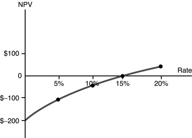
Figure S2.1 graphs NPV versus the discount rate. The IRR on this project is approximately 15.8 percent.
At an opportunity cost of capital of 10 percent, the project has a negative NPV; therefore, it should be rejected (even though the IRR is greater than the cost of capital).
This is an interesting example which demonstrates another difficulty with the IRR technique; namely, that it does not consider the order of cash flows.
Chapter 2 Investment Decisions: The Certainty Case 9
CF 3,000(1 .4) .4(2,000) 2,600
NPV 10,000 2,600(2.991) 2,223.40
Discounted Cash Flows @ 0% @ 10% @ 15% @ 16% @ 20% 400 363.64 347.83 344.83 333.33 400 330.58 302.46 297.27 277.78 1,000 751.32 657.52 640.66 578.70 200 57.10 7.23 1.44 32.41
1
a second
Figure S2.1 The internal rate of return ignores the order of cash flows
There is
IRR at 315.75%,
but it has no economic meaning. Note also that the function is undefined at IRR
1.
7. These are the cash flows for project A which was used as an example in section E of the chapter. We are told that the IRR for these cash flows is 200%. But how is this determined? One way is to graph the NPV for a wide range of interest rates and observe which rates give NPV 0. These rates are the
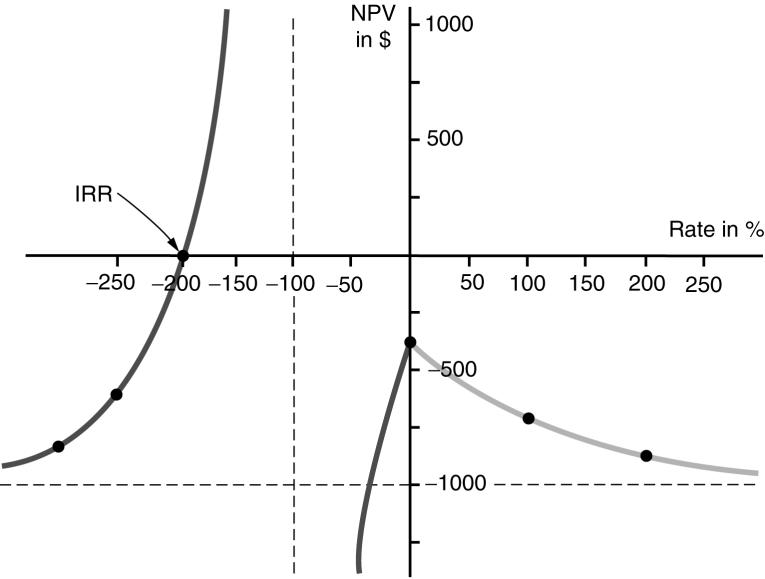
Figure S2.2 An
calculation internal rates of return for the project. Figure S2.2 plots NPV against various discount rates for this particular set of cash flows. By inspection, we see that the IRR is
8. All of the information about the financing of the project is irrelevant for computation of the correct cash flows for capital budgeting. Sources of financing, as well as their costs, are included in the computation of the cost of capital. Therefore, it would be “double counting” to include financing costs (or the tax changes which they create) in cash flows for capital budgeting purposes.
The cash flows are:
cc (RevVCFCCdep)(1)dep(200(360)00)(1.4).4(400)
= 496 (PVIFa: 10%, 3 years)* – 1,200 = 496 (2.487) – 1,200 = 33.55
The project should be accepted.
9. First calculate cash flows for capital budgeting purposes:
CF(RevVC)(1)dep (0(290))(1.5).5(180)
* Note: PVIFa: 10%, 3 years, the discount factor for a three year annuity paid in arrears (at 10%).
10 Copeland/Shastri/Weston • Financial Theory and Corporate Policy, Fourth Edition
IRR
336160 496
NPV
tttcc
14590235
Next, calculate the NPV:
The project should be rejected because it has negative net present value.
10. The net present values are calculated below:
Project A has a two-year payback.
Project B has a one-year payback.
Project C has a three-year payback.
Therefore, if projects A and B are mutually exclusive, project B would be preferable according to both capital budgeting techniques.
Project (A C) has a two-year payback, NPV $1.15.
Project (B C) has a three-year payback, NPV $1.91.
Once Project C is combined with A or B, the results change if we use the payback criterion. Now A C is preferred. Previously, B was preferred. Because C is an independent choice, it should be irrelevant when considering a choice between A and B. However, with payback, this is not true. Payback violates value additivity. On the other hand, NPV does not. B C is preferred. Its NPV is simply the sum of the NPV’s of B and C separately. Therefore, NPV does obey the value additivity principle.
11. Using the method discussed in section F.3 of this chapter, in the first year the firm invests $5,000 and expects to earn IRR. Therefore, at the end of the first time period, we have 5,000(1 IRR)
During the second period the firm borrows from the project at the opportunity cost of capital, k. The amount borrowed is
(10,000 5,000(1 IRR))
Chapter 2 Investment Decisions: The Certainty Case 11
5 t 0 t t1 t0 CF NPVI (1WACC) (CF)(presentvalueannuityfactor@10%,5years) I 235(3.791)900.00 890.89900.009.12
Year PVIF A PV (A) B PV (B) C PV (C) A C B C 0 1.000 1 1.00 1 1.00 1 1.00 2 2 1 .909 2 .826 3 .751 1 .75 .75 2.25 .10 NPV(A C) 1.15 NPV(B C) 1.91
12 Copeland/Shastri/Weston • Financial Theory and Corporate Policy, Fourth Edition
(10,000 5,000(1 IRR)) (1 k)
3,000 at the
of the
3,000 (10,000 5,000(1 IRR)) (1.10) Solving for IRR, we have 3,000 1.10 10,000 1IRR45.45% 5,000 Financial Theory and Corporate Policy international 4th Edition Copeland Solutions Manual Full Download: http://testbanktip.com/download/financial-theory-and-corporate-policy-international-4th-edition-copeland-solutions-manual/ Download all pages and all chapters at: TestBankTip.com
By the end of the second time period this is worth
The firm then lends
end
second time period:
