Solution manual for fundamentals of communication systems 2nd edition by proakis salehi isbn 0133354 by angie.coleman600

Solution Manual for Fundamentals of Communication Systems 2nd Edition by Proakis Salehi ISBN 0133354857 9780133354850

Full link download

Solution Manual

https://testbankpack.com/p/solution-manual-for-fundamentals-ofcommunication-systems-2nd-edition-by-proakis-salehi-isbn0133354857-9780133354850/

Chapter 2

Problem 2.1

1. Π(2t+ 5)= Π 2 5 + This indicates first we have to plot Π(2t)and then shift it to left t 2 by 5 A plot is shown below:

Λ(t n)is a sum of shifted triangular pulses Note that the sum of the left and right side of triangular pulses that are displaced by one unit of time is equal to 1, The plot is given below

n=0

3. It is obvious from the definition of sgn(t)that sgn(2t)= sgn(t) Therefore x3(t)= 0.

3 2 +

Π (2t 5) ✻ 1 ✲ t 11 9 P∞

4 4

✻ 1 ✲ t 1

(t)

1 0.8 0.6 0.4 0.2 0 −0.2 −0.4 −1 −0.8 −0.6 −0.4 −0.2 0 0.2 0.4 0.6 0.8 1

4. x4(t)is sinc(t)contracted by a factor of 10.

5 2 1 1 3 4 Problem 2.2 1. x[n]= sinc(3n/9)= sinc(n/3) . 1 0.8 0.6 0.4 0.2 0 −0.2 −0.4 −20 −15 −10 −5 0 5 10 15 20 2. x[n]= Π n 4 If 1 ≤ n 1 3 ≤ 2, i.e., 2 ≤ n≤ 10, we have x[n] = 1. 1 0.9 0.8 0.7 0.6 0.5 0.4 0.3 0.2 0.1 0 −20 −15 −10 −5 0 5 10 15 20 3. x[n]= nu (n/4) (n 1)u (n/4 1) . For n<0, x[n]= 0, for 0 ≤ n≤ 3, x[n] = n and 4 1 4 1 4 for n≥ 4, x[n]= n n + 1 = 1. 4 4

Problem 2.3

x1[n]= 1 and x2[n]= cos(2πn)= 1, for all n This shows that two signals can be different but their sampled versions be the same.

Problem 2.4

Let x1[n] and x2[n] be two periodic signals with periods N1 and N2, respectively, and let N = LCM(N1,N2) , and define x[n]= x1[n]+x2[n] Then obviously x1[n+N]= x1[n]and x2[n+N]= x2[n], and hence x[n] = x[n+ N],i.e., x[n]is periodic with period N. For continuous-time signals x1(t)and x2(t)with periods T1 and T2 respectively, in general we cannot find a T such that T = k1T1 = k2T2 for integers k1 and k2 This is obvious for instance if T1 = 1 and T2 = π The necessary and sufficient condition for the sum to be periodic is that T1 be a rational number.

Problem 2.5

Using the result of problem 2 4 we have:

1. The frequencies are 2000 and 5500, their ratio (and therefore the ratio of the periods) is rational, hence the sum is periodic.

2. The frequencies are 2000 and 5500 . Their ratio is not rational, hence the sum is not periodic.

3. The sum of two periodic discrete-time signal is periodic.

6 T2 π 1 0.9 0.8 0.7 0.6 0.5 0.4 0.3 0.2 0.1 0 −5 0 5 10 15 20

4. The fist signal is periodic but cos[11000n] is not periodic, since there is no N such that cos[11000(n+ N)]= cos(11000n)for all n Therefore the sum cannot be periodic.

Thus, x1(t)is an odd signal

t +

Therefore

isneither even norodd. We have cos

This part can also be considered as a special case of part 7 of this problem)

Hence, the signal x3(t)is even.

The signal x4(t)is neither even nor odd. The even part of the signal is

7 ⇒ t t t t ⇒ ⇒ ⇒ =

Problem 2.6 1) x1(t)= e t t >0 et t <0 0 t = 0 = x1( t)= e t t >0 et t <0 0 t = 0 = x1(t)

2) x

πt + π = cos π cos(120πt) 1 3 3 3 sin π sin(120πt)

x2e(t) = cos π cos(120πt) and x2o(t)= sin π sin(120πt) 3 3 3 (Note:

3) x3(t)= e |t| = x3( t)= e |( t)| = e |t| = x3(t)

2(t)= cos 20

120

4) x4(t)= t t ≥ 0 0 t <0 = x4( t)= 0 t ≥ 0 t t <0

x4,e(t)= x4(t)+ x4( t) 2 = 2 t ≥ 0 2 t <0 |t| = 2 The odd

is 5) x4,o(t)= x4(t) x4( t) 2 = 2 t ≥ 0 t 2 t <0 2 x5(t)= x1(t) x2(t) = x5( t)= x1( t) x2( t)= x1(t)+ x2(t) Clearly x5( t) ≠ x5(t)

x2(t)= 0 ∀t Similarly x5( t)≠ x5(t) since otherwise x1(t)= 0 ∀t. The even and the odd parts of x5(t)are given by x5(t)+ x5( t) x5,e(t) = x5,o(t) = 2 = x1(t) x5(t) x5( t) 2 = x2(t)

part

since otherwise

For the first two questions we will need the integral

9 1 T 1 = 2 T = 2 = = = = = 1 2 8 = 2

Problem 2.7

R eax cos2 xdx I 1 Z cos 2 a x deax 1 ax = a e cos 2 1 Z x + a eaxsin2x dx 1 eax a cos 2 1 Z x + a2 sin2x deax 1 eax a 1 ax cos 2 2 1 ax x + a2e 1 ax 2 Z sin2x a2 2 Z eax ax cos2x dx 2 e a 1 ax cos 2 x + a2e 1 ax sin2x a2 2 Z e (2cos ax x 1)dx 4 Thus, e cos a x + a2e sin2x a2 e dx a2I 1 2 2 ax I= 4 + a2 (acos x + sin2x)+ a e 1) T Z 2 Ex = lim T T→∞ 2 T Z 2 x2(t)dx= lim →∞ 0 e 2tcos 2 tdt T = lim h ( 2cos 2 t+ sin2t) i 2 e 2t T→∞ 8 0 1 T 3 lim T→∞ 8 ( 2cos 2 + sin T 1)e T + 3 =

1(t)

energy-type signal

the energy content is 3/8 2) Ex = lim T→∞ T Z 2 T 2 Z 0 T Z 2 x2(t)dx lim T →∞ 2 T Z 2 e 2tcos 2 tdt = lim T→∞ e 2tcos 2 tdt T 2 e 2t cos 2 tdt 0 But, Z 0 1 h i 0 lim T→∞ e 2t cos 2 tdt lim T T→∞ 8 ( 2cos 2 t + sin2t) 1 e 2t T

Thus x

is an

and

since 2+ cosθ+ sinθ>0. Thus, Ex =∞ since as we have seen from the first question the second integral is bounded. Hence, the signal x2(t) is not an energy-type signal To test if x2(t) is a power-type signal we find Px

1 0 T 2 = lim 1 3+ (2cos 2 + 1+ sinT)eT = ∞ T→∞ 8 2

Px = lim 1 Z 0 e 2tcos 2 dt + lim T 1 Z 2 e 2tcos 2 dt T→∞ T T T→∞ T 0

1 1 →∞ T 3 T 1 k T 2 = 2 2 2 2 2 2 1 2 T 2 T 2 T But limT 1 R 2 e 2tcos2 dt is zero and 0 lim 1 Z 0 e 2tcos 2 dt = lim 1 2cos 2 + 1+ sinT eT T→∞ T T T→∞ 8T 2 1 1 > lim T→∞ T

3) eT > lim T→∞ T(1+ T+ T2)> lim T = ∞ T→∞ T Z 2 Ex = lim T T→∞ 2 T Z 2 x2(t)dx lim T →∞ 2 T T Z 2 sgn 2(t)dt= lim T→∞ T T dt = lim T =∞ T→∞ Px = lim 1 Z 2 sgn 2(t)dt= lim 1 Z 2 dt = lim 1 T = 1 T→∞ T T T→∞ T T T→∞ T

so that T Z 2 lim T→∞ T Acos(2πft)dt= ∞ X k=−∞ Z k+ 2f A 1 2f cos(2πft)dt= 0 T Z 2 lim A2 cos 2(2πft)dt = lim T 1 Z 2 (A2+ A2 cos(2π2ft))dt T→∞ T T→∞ 2 T T = lim 1 Z 2 A2dt = lim A2T = ∞ T→∞ 2 T T→∞ 2 Ex = lim T→∞ T Z 2 (A2 cos 2(2πf1t)+ B2 cos 2(2πf2t)+ 2AB cos(2πf1t)cos(2πf2t))dt 2 T T Z 2 Z 2 = lim T→∞ A2 cos 2(2πf1t)dt+ lim T T→∞ T B2 cos 2(2πf2t)dt+ 2 Z 2 AB lim T→∞ T[cos 2(2π(f1 + f2)+ cos 2(2π(f1 f2)]dt = ∞ +∞ + 0 = ∞

Thus the signal x

(t)is not a power-type signal.

The signal x3(t)is of the power-type and the power content is

4) First note that

Thus the signal is not of the energy-type. To test if the signal is of the power-type we consider two cases f1 = f2 and f1 ≠ f2 In the first case

1 2 = + 1 +

Px = lim T 1 Z 2 (A+ B)2 cos 2(2πf1)dt T→∞ T 1 lim T→∞ 2T T 2 T Z 2 (A B)2 T 2 dt = (A B)2 2

Thus the signal is of the power-type and if f1 = f2 the power content is (A+ B)2/2 whereas if f1 ≠ f2 the power content is 1(A2+ B2)

Problem 2.8

1. Let x(t)= 2Λ t Λ(t) , then x1(t)= P∞ x(t 4n) First we plot x(t)then by shifting 2 n=−∞ it by multiples of 4 we can plot x1(t) x(t) is a triangular pulse of width 4 and height 2 from which a standard triangular pulse of width 1 and height 1 is subtracted. The result is a trapezoidal pulse, which when replicated at intervals of 4 gives the plot of x1(t) .

2. This is the sum of two periodic signals with periods 2π and 1. Since the ratio of the two periods is not rational the sum is not periodic (by the result of problem 2.4)

3. sin[n]is not periodic. There is no integer N such that sin[n+ N]= sin[n]for all n Problem

is a power-type signal and its power content is A2

1 3 2 2 2 1 2 2 2 If f1 ≠ f2 then Px = lim T 1 Z 2 (A2 cos 2(2πf1t)+ B2 cos 2(2πf2t)+ 2AB cos(2πf1t)cos(2πf2t))dt T→∞ T T = lim 1 " A2T + B2T # = A2 B2 + T→∞ T 2 2 2 2

x1(t) ✻ 1 ✲ t 6 2 2 6

2.9 1) Px = lim T 1 Z 2 A2 ej(2πf0t+θ) dt = lim T 1 Z 2 A2dt = lim A2T = A2 T→∞ T T T→∞ T T T→∞ T

x(t)= Aej(2πf0t+θ

2) Px = lim T 1 Z 2 A2 cos 2(2πf0t+ θ)dt = lim T 1 Z 2 A2 dt + lim T 1 Z 2 A2 cos(4πf0t+ 2θ)dt T→∞ T T T→∞ T T 2 2 T→∞ T T 2 2

Thus

)

As T → ∞ , the there will be no contribution by the second integral Thus the signal is a power-type signal and its power content is A

1 1 2 2

Thus the unit step signal is a power-type signal and its power content is 1/2

Thus the signal is not an energy-type signal

Since Px is not bounded away from zero it follows by definition that the signal is not of the power- type (recall that power-type signals should satisfy 0 <Px <∞).

The even and the odd part of x(t)are given by

10 1 = = 2 2 ⇒ 3) Px = lim T 1 Z 2 u2 (t)dt = lim T 1 Z 2 dt = lim 1 T 1 = T→∞ T T 1 T→∞ T 0 T→∞ T 2 2

4) T T Z 2 Z 2 1 1 T/2 Ex = lim x2(t)dt= lim K2t 2 dt= lim 2K2t2 T→∞ T √ 1 T→∞ 0 T→∞ 0 = lim T→∞ 2K2T 2 = ∞

Px = lim T 1 Z 2 x2(t)dt= lim T 1 Z 2 K2t 2 dt T→∞ T 1 T 2 1 T/2 T→∞ T 0 1 1 √ 1 lim T→∞ T 2K2t2 0 lim T→∞ T 2K2(T/2)2 = lim T→∞ 2K2T 2 = 0

Problem 2.10 t+ 1, 1 ≤ t ≤ 0 1 t >0 Λ(t)= t+ 1, 0 ≤ t ≤ 1 u 1(t)= 1/2 t = 0 0, o.w 0 t <0 Thus,

x(t)= Λ(t)u 1(t)is given by x(t)= 0 t <0 1/2 t = 0 t+ 1 0 ≤ t ≤ 1 0 t ≥ 1 = x( t)= 0 t ≤ 1 t + 1 1 ≤ t <0 1/2 t = 0 0 t >0

x(t)

the signal

+ x(

11 t 1 t+1 xe(t) = 2 = 2 Λ(t) xo(t) = x(t) x( t) 2 = 0 t ≤ 1 2 1 ≤ t <0 0 t = 0 2 0 <t ≤ 1 0 1 ≤ t

Problem 2.11

1) Suppose that

Thus x1(t)= x2(t)and x1(t)= x(t) x

= x1(t)x2(t) = z( t)= x1( t)x2( t)= ( x1(t))( x2(t))= z(t) o o ⇒ o o o o

Thus the product of two even or odd signals is an even signal. For v(t) = x1(t)x1(t)we havee o

v( t)= x1( t)x1( t)= x1(t)( x1(t))= x1(t)x1(t)= v(t) e o e o e o

Thus the product of an even and an odd signal is an odd signal.

3) One trivial example is t + 1 and t t+1

Problem 2.12

1) x1(t)= Π(t)+ Π( t) . The signal Π(t)is even so that x1(t)= 2Π(t)

12 2

x(t)= x1(t)+ x1(t)= x2(t)+ x2(t) e o e o

x( t) = x1(t) x1(t)

o x 1

x(t)+ x( t) e(t) = 2 x2 2 2 2 e(t)+ xo(t)+ xe( t)+ xo( t) = 2 2x2(t)+ x2(t) x2(t) e o o 2 = 2 = xe(t)

with x1(t), x2(t)even signals and x1(t), x1(t)odd signals. Then,

so that

o e o

2(t)

1(t)= x(t) x

= x

e e o e e o

1(t), x2(t)be two odd signals Then, e

o o y(t) = x1(t)x2(t) = y( t)= x1( t)x2( t)= x1(t)x2(t)= y(t) e e ⇒ e e e e z(t)

2) Let x1(t), x2(t)be two even signals and x

2 1 1 1 2 2

13 n=−∞ 1 2) x2(t)= Λ(t)· Π(t)= 0, t < 1/2 1/4, t = 1/2 t + 1, 1/2 <t ≤ 0 t+ 1, 0 ≤ t <1/2 1/4, t = 1/2 0, 1/2 <t 1 . . . 1 . . . . . .4. . . . 1 1 2 2 3) x3(t)= P∞ Λ(t 2n) 1 ... ... 3 1 1 3 4) x4(t)= sgn(t)+ sgn(1 t) Note that x4(0)= 1, x4(1)= 1 2 . . . . 0 5) x5(t)= sinc(t)sgn(t) Note that x5(0)= 0.

Problem 2.13

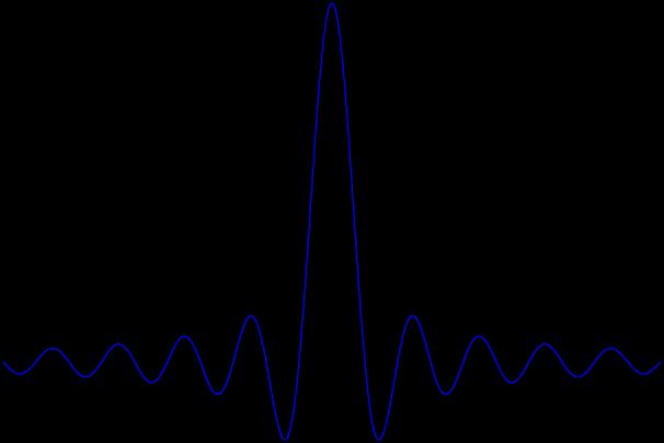
1) The value of the expression sinc(t)δ(t)can be found by examining its effect on a function φ(t) through the integral

Thus sinc(t)δ(t)has the same effect as the function sinc(0)δ(t)and we conclude that

14 X X 1 0.8 0.6 0.4 0.2 0 -0.2 -0.4 -0.6 -0.8 -1 -4 -3 -2 -1 0 1 2 3 4

Z ∞ Z ∞ φ(t)sinc(t)δ(t)= φ(0)sinc(0)= sinc(0) ∞ ∞φ(t)δ(t)

x1(t)= sinc(t)δ(t)= sinc(0)δ(t)= δ(t) 2) sinc(t)δ(t 3)= sinc(3)δ(t 3)= 0. 3) x3(t) = Λ(t)⋆ ∞ X n=−∞ δ(t 2n) ∞ Z ∞ = n=−∞ ∞ ∞ Z ∞ = n=−∞ ∞ ∞ X Λ(t τ)δ(τ 2n)dτ Λ(τ t)δ(τ 2n)dτ = n=−∞ Λ(t 2n)

Problem 2.14

The impulse signal can be defined in terms of the limit

is an even function for every τ so that δ(

is even Since

t)is even, we obtain

Thus, the function

is odd. For the function δ(n)(t)we have

15 1 τ=0 1 ⇒ | d 4) x4(t) = Λ(t)⋆δ ′ (t)= d Z ∞ Λ(t τ)δ ′ (τ)dτ ∞ 0 t < 1 2 t = 1 1 1 <t <0 = ( 1)dτ Λ(t τ) = Λ ′ (t)= 0 t = 0 1 0 <t <1 2 t = 1 0 1 <t 5) x5(t)= cos t+ π δ(3t)= 1 cos t + π δ(t)= 1 cos π δ(t). Hence x5(t)= 1δ(t) . 2 3 3 2 3 3 3 6 6) 1 1 1 x6(t)= δ(5t)⋆δ(4t)= 5 δ(t)⋆ 4δ(t)= 20 δ(t) 7) Z ∞ sinc(t)δ(t)dt= sinc(0)= 1 ∞ 8) Z ∞ sinc(t+ 1)δ(t)dt= sinc(1)= 0 ∞

1 δ(t)= lim |t| e τ t| But e τ→0 2τ

τ δ(t)= δ( t) = δ ′ (t)= δ ′ ( t)

δ(

Z ∞ φ(t)δ(n)( t)dt= ( 1)n ∞ Z ∞ φ(t)δ(n)(t)dt ∞

δ′(t)

where we have used the differentiation chain rule

16 d =

δ(k 1)( t) dt d d( t)δ(k 1)( t)dt( t)= ( 1)δ(k)( t)

Thus, if n= 2l(even)

and the function δ

is even If n

from which we conclude that δ(n)(t)is odd.

The signal δ(n)(t)is even if nis even and odd if nis odd. Consider first the case that n= 2l Then,

If nis odd then,

Problem 2.16

1) Nonlinear, since the response to x(t)= 0 is not y(t) = 0 (this is a necessary condition for linearity of a system, see also problem 2.21).

Z ∞ φ(t)δ(n)( t)dt= ∞ Z ∞ φ(t)δ(n)(t)dt ∞

( 1)n = 1 and Z ∞ Z ∞ φ(t)δ(n)( t)dt= ∞ ∞φ(t)δ(n)(t)dt

(n)(t)

= 2

1 (odd), then

Problem

x(t)⋆δ(n)(t)= Z ∞ x(τ)δ(n)(t τ)dτ ∞

2.15

x(t)⋆δ(2l)(t)=

Z ∞ x(τ)δ(2l)(τ t)dτ = ( 1)2l ∞ d2l dτ2lx(τ) = τ=t dn dtnx(t) x(t)⋆δ(2l+1)(t) = Z ∞ x(τ)( 1)δ(2l+1)(τ t)dτ = ( 1)( 1)2l+1 ∞ dn d2l+1 dτ2l+1 x(τ) τ=t = dtnx(t) In both cases x(t)⋆δ(n)(t)= dn dtnx(t) The convolution of x(t)with u 1(t)is x(t)⋆u 1(t)= But u 1(t τ)= 0 for τ >t

Z ∞ x(τ)u 1(t τ)dτ ∞ Z t x(t)⋆u 1(t)= x(τ)dτ ∞

so that

2) Nonlinear, if we multiply the input by constant 1, the output does not change. In a linear system the output should be scaled by 1.

3) Linear, the output to any input zero, therefore for the input αx1(t)+ βx2(t) the output is zero which can be considered as αy1(t)+ βy2(t)= α× 0+ β× 0 = 0. This is a linear combination of the corresponding outputs to x1(t)and x2(t) .

4) Nonlinear, the output to x(t)= 0 is not zero

5) Nonlinear. The system is not homogeneous for if α <0 and x(t)>0 then y(t)= T[αx(t)] = 0 whereas z(t)= αT[x(t)]= α

6) Linear For if x(t) = αx1(t)+ βx2(t)then

T[αx1(t)+ βx2(t)] = (αx1(t)+ βx2(t))e t = αx1(t)e t + βx2(t)e t = αT[x1(t)]+ βT[x2(t)]

7) Linear For if x(t) = αx1(t)+ βx2(t)then T[αx1(t)+ βx2(t)] = (αx1(t)+ βx2(t))u(t) = αx1(t)u(t)+ βx2(t)u(t)= αT[x1(t)]+ βT[x2(t)]

8) Linear We can write the output of this feedback system as

Then for x(t) = αx1(t)+ βx2(t)

9) Linear. Assuming that only a finite number of jumps occur in the interval ( ∞,t]and that the magnitude of these jumps is finite so that the algebraic sum is well defined, we obtain

= T[αx(t)]=

where N is the number of jumps in ( ∞,t]and Jx(tn)is the value of the jump at time instant tn, that is Jx(tn) = lim(x(tn+ ǫ) x(tn ǫ))

For x(t)= x1(t)+ x2(t)we can assume that x1(t), x2(t)and x(t)have the same number of jumps and at the same positions. This is true since we can always add new jumps of magnitude zero to the already existing ones. Then for each tn, Jx(tn)= Jx1(tn)+ Jx2(tn) and

that the system is additive.

y(t) = x(t)+ y(t 1)=

∞ X x(t n) n=0 y(t) = ∞ X (αx

(t n)+ βx2(t n)) n=0 ∞ ∞ = α X

+ β X x

(t n)) n=0 = αy1(t)+ βy2(t) n=0

x1(t n)

N N y(t)

X α

n)= α X Jx(tn)= αT[x(t)] n=1 n=1

→0

N N N y(t)

+ X

= X Jx

X Jx (t

)

(tn)

20 n=1 1 n= 1 2 n=1

Problem 2.17

Only if ( = ) ⇒

If the system T is linear then

T [αx1(t)+ βx2(t)]= αT [x1(t)]+ βT[x2(t)] for all α, βand x(t)’s. If we set β= 0, then

T [αx1(t)]= αT [x1(t)] so that the system is homogeneous If we let α = β= 1, we obtain

T [x1(t)+ x2(t)]= T [x1(t)]+T [x2(t)] and thus the system is additive. If ( = ) Suppose that both conditions 1) and 2) hold. Thus the system is homogeneous and additive. Then

T [αx1(t)+ βx2(t)]

= T [αx1(t)]+ T [βx2(t)](additive system)

= αT[x1(t)]+ βT[x2(t)](homogeneous system)

Thus the system is linear

Problem 2.18

1. Neither homogeneous nor additive.

2. Neither homogeneous nor additive.

3. Homogeneous and additive.

4. Neither homogeneous nor additive.

5. Neither homogeneous nor additive.

6. Homogeneous but not additive.

7. Neither homogeneous nor additive.

8. Homogeneous and additive.

9. Homogeneous and additive.

21 ⇐

10. Homogeneous and additive.

11. Homogeneous and additive.

12. Homogeneous and additive.

13. Homogeneous and additive.

14. Homogeneous and additive.

Problem 2.19

We first prove that

T [nx(t)]= nT [x(t)] for n∈N The proof is by induction on n For n= 2 the previous equation holds since the system is additive. Let us assume that it is true for nand prove that it holds for n+ 1.

T [(n+ 1)x(t)]

= T [nx(t)+ x(t)]

= T [nx(t)]+ T [x(t)](additive property of the system)

= nT [x(t)]+ T [x(t)](hypothesis, equation holds for n)

= (n+ 1)T [x(t)]

Thus T [nx(t)]= nT [x(t)]for every n. Now, let

= my(t) This implies that

T m = T [y(t)]

and since T [x(t)]= T [my(t)]= mT[y(t)] we obtain

1 = m T [x(t)]

Thus, for an arbitrary rational α = k we have

x(t) k

= kT λ = λ T [x(t)] Problem 2.20

Clearly, for any α

= T k

22 λ α x (t) αx (t) T λ

x(t)

k x(t)

x(t)

2 2 2 y(t)= T[αx(t)]= αx ′(t) x ′ (t)≠ 0 = 0 x ′(t)= 0 x ′(t) x ′(t)≠ 0 0 x ′(t)= 0 = αT[x(t)]

Thus the system is homogeneous and if it is additive then it is linear However, if x(t)

x1(t)+ x2(t)then x ′(t)= x ′ (t)+ x ′ (t) and 1 2

Thus T[x1(t)+ x2(t)]≠ T[x1(t)]+ T[x2(t)]unless c = 0. Hence the system is nonlinear since the additive property has to hold for every x1(t)and x2(t)

As another example of a system that is homogeneous but non linear is the system described by

Problem 2.21

Any zero input signal can be written as 0 x(t)with x(t)an arbitrary signal Then, the response of the linear system is y(t)= L[0 · x(t)]and since the system is homogeneous (linear system) we obtain

y(t)= L[0· x(t)]= 0· L[x(t)]= 0

Thus the response of the linear system is identically zero

Problem 2.22

For the system to be linear we must have T [αx1(t)+ βx2(t)]= αT [x1(t)]+ βT[x2(t)]

for every α, βand x(t)’s

T [αx1(t)+ βx2(t)] = (αx1(t)+ βx2(t))cos(2πf0t)

= αx1(t)cos(2πf0t)+ βx2(t)cos(2πf0t)

= αT[x1(t)]+ βT[x2(t)]

Thus the system is linear In order for the system to be time-invariant the response to x(t t0) should be y(t t0)where y(t)is the response of the system to x(t) Clearly y(t t0)= x(t t0)cos(2πf0(t t0))and the

23 ≠ 1 2 x ′ 1 1 1 ′

(x1(t)+

2(t))2 x2(t) x2(t) 1(t)+ x2(t) x1(t) + x2(t) x ′ ′ ′ ′ for

and T[x1(t)

= (x1(t)+ c)2 1(t) = x2(t)+ 2cx1(t)+ c2 x ′ (t) T[x1(t)]+ T[x

(t)]= x2(t) x1(t)

some x1(t), x2(t) To see this let x2(t)= c (a constant signal) Then

+ x2(t)]

T[x(t)]= x(t)

Clearly T[αx(t)]= αT[x(t)]but T[x1(t)+ x2(t)]≠ T[x1(t)]+ T[x2(t)]

+ x(t 1) x(t)x(t 1)>0 0 otherwise

response of the system to x(t t0)is y ′(t) = x(t t0)cos(2πf0t) Since cos(2πf0(t t0)) is not equal to cos(2πf0t)for all t, t0 we conclude that y ′(t)≠ y(t t0) and thus the system is time-variant.

Problem 2.23

1) False. For if T1[x(t)] = x3(t)and T2[x(t)] = x1/3(t)then the cascade of the two systems is the identity system T[x(t)]= x(t)which is known to be linear However, both T1[ ]and T2[ ]are nonlinear

2) False. For if T1[x(t)]= tx(t) t ≠ 0 0 t = 0 T2[x(t)]= 1x(t) t ≠ 0 0 t

Then T2[T1[x(t)]]= x(t) and the system which is the cascade of T1[·]followed by T2[·]is time- invariant , whereas both T1[·]and T2[·]are time variant

3) False. Consider the system y(t)= T[x(t)]= x(t) t ≥ 0 1 t <0

Then the output of the system y(t)depends only on the input x(τ)for τ ≤ t This means that the system is causal However the response to a causal signal, x(t)= 0 for t ≤ 0, is nonzero for negative values of t and thus it is not causal

Problem 2.24

1) Time invariant: The response to x(t t0)is 2x(t t0)+ 3 which is y(t t0) .

2) Time varying the response to x(t t0)is (t+ 2)x(t t0)but y(t t0)= (t t0 + 2)x(t t0) , obviously the two are not equal.

3) Time-varying system The response y(t t0)is equal to x( (t t0))= x( t + t0) However the response of the system to x(t t0)is z(t)= x( t t0)which is not equal to y(t t0)

4) Time-varying system Clearly y(t)= x(t)u 1(t) = y(t t0)= x(t t0)u 1(t t0)

However, the response of the system to x(t t0)is z(t)= x(t t0)u 1(t)which is not equal to y(t t0)

5) Time-invariant system. Clearly y(t)=

t ⇒ ⇒

Z t x(τ)dτ = ∞ y(t t0)=

The response of the system to x(t t0)is Z t Z t t0

Z t t0 ∞ x(τ)dτ

= 0

21 z(t)= x(τ t0)dτ= ∞ x(v)dv= y(t t0) ∞

where we have used the change of variable

6) Time-invariant system Writing y(t)as

we get

Problem 2.25

The differentiator is a LTI system (see examples 2 19 and 2 1 21 in book) It is true that the output of a system which is the cascade of two LTI systems does not depend on the order of the systems This can be easily seen by the commutative property of the convolution

Let h1(t)be the impulse response of a differentiator, and let y(t)be the output of the system h2(t) with input x(t) Then,

Problem 2.26

The integrator is is a LTI system (why?) It is true that the output of a system which is the cascade of two LTI systems does not depend on the order of the systems. This can be easily seen by the commutative property of the convolution

Let h1(t)be the impulse response of an integrator, and let y(t)be the output of the system h2(t) with input x(t) Then,

Problem 2.27

The output of a LTI system is the convolution of the input with the impulse response of the system. Thus,

22 n

τ t0

v =

P∞ =−∞ x(t n)

y(t t0)= ∞ X n=−∞ x(t t0 n)= T[x(t t0)]

h1(t)⋆h2(t)= h2(t)⋆h1(t)

z(t) = h2(t)⋆x ′ (t)= h2(t)⋆(h1(t)⋆x(t)) = h2(t)⋆h1(t)⋆x(t)= h1(t)⋆h2(t)⋆x(t) = h1(t)⋆y(t)= y ′ (t)

h1(t)⋆h2(t)= h2(t)⋆h1(t)

z(t) = h2(t)⋆ Z t x(τ)dτ = h2(t)⋆(h1(t)⋆x(t)) ∞ = h2(t)⋆h1(t)⋆x(t)= h1(t)⋆h2(t)⋆x(t) Z t = h1(t)⋆y(t)= y(τ)dτ ∞

23 1 δ(t)= Z ∞ h(τ)e α(t τ)u ∞ (t τ)dτ= Z t h(τ)e α(t τ)dτ ∞

Differentiating both sides with respect to t we obtain

The response of the system to the input x(t) is

Problem 2.28

For the system to be causal the output at the time instant t0 should depend only on x(t)for

We observe that the second integral on the right side of the equation depends on values of x(τ)for τ greater than t0. Thus the system is non causal.

Problem 2.29

Consider the system

This system is causal since the output at the time instant t depends only on values of x(τ) for τ ≤ t (actually it depends only on the value of x(τ)for τ = t, a stronger condition.) However, the response of the system to the impulse signal δ(t)is one for t < 0 so that the impulse response of the system is nonzero for t <0.

Problem 2.30

Z t d " Z t # δ ′ (t) = ( α)e αt h(τ)eατdτ + e αt ∞ dt h(τ)eατdτ ∞ = ( α)δ(t)+ e αth(t)eαt = ( α)δ(t)+ h(t) Thus h(t)= αδ(t)+ δ ′ (t)

y(t) = Z ∞ x(τ) αδ(t τ)+ δ ′ (t τ) dτ ∞ Z ∞ = α x(τ)δ(t τ)dτ+ ∞ d Z ∞ x(τ)δ ′ (t τ)dτ ∞ = αx(t)+ dtx(t)

≤ t0

1 y(t0)= 2T Z t0+T t0 T x(τ)dτ = 1 Z t0 2T t0 T x(τ)dτ+ 1 Z t0+T 2T t0 x(τ)dτ

y(t)= T[x(t)]= x(t) x(t)≠ 0 1 x(t)= 0

1. Noncausal: Since for t <0 we do not have sinc(t)= 0.

2. This is a rectangular signal of width 6 centered at t0 = 3, for negative t’s it is zero, therefore the system is causal

3. The system is causal since for negative t’s h(t)= 0.

Problem 2.31

The output y(t)of a LTI system with impulse response h(t)and input signal u 1(t)is

But u 1(t τ)= 1 for τ <t so that

Similarly, since u 1(t τ)= 0 for τ <t we obtain

Combining the previous integrals we have

Problem 2.32

Let h(t)denote the the impulse response of a differentiator Then for every input signal

If x(t)= δ(t)then the output of the differentiator is its impulse response. Thus, δ(t)⋆h(t)= h(t)= δ ′ (t)

The output of the system to an arbitrary input x(t)can be found by convolving x(t)with δ′(t) In this case

Assume that the impulse response of a system which delays its input by t0 is h(t) Then the response to the input δ(t) is

δ(t)⋆h(t)= δ(t t0)

However, for every x(t)

δ(t)⋆x(t)= x(t)

so that h(t)= δ(t t0) The output of the system to an arbitrary input x(t) is

y(t)= Z ∞ h(τ)u 1(t τ)dτ= ∞ Z t h(τ)u 1(t τ)dτ+ ∞ Z ∞ h(τ)u 1(t τ)dτ t

Z t h(τ)u 1(t τ)dτ= ∞

Z ∞ Z t h(τ)dτ ∞ h(τ)u 1(t τ)dτ= 0 t

Z ∞ Z t y(t)= h(τ)u 1(t τ)dτ= ∞ h(τ)dτ ∞

d x(t)⋆h(t)

dtx(t)

y(t)

⋆δ

Z ∞ x(τ)δ ′ (t τ)dτ= ∞ dx(t)dt

= x(t)

′ (t)=

27 Z ∞ y(t) = x(t)⋆δ(t t0)= x(τ)δ(t t0 τ)dτ= x(t t0) ∞

The response of the system to the signal

Thus the system is linear. The response to x(t t0)is

where we have used the change of variables v = τ t0 Thus the system is time invariant The impulse response is obtained by applying an impulse at the input

28 1 1 1 1 1 1 ⇒ ⇒ 2 2 1 2 2 2

Problem 2.33

αx1

y1(t)= Z t t T (αx1(τ)+ βx2(τ))dτ= α Z t t T x1(τ)dτ+ β Z t t T x2(τ)dτ

(t)+

x2(t)is

y1(t)= Z t t T x(τ t0)dτ= Z t t0 t t0 T x(v)dv = y(t t0)

h(t)= Z t t T δ(τ)dτ= Z t δ(τ)dτ ∞ Z t T ∞ δ(τ)dτ= u 1(t) u 1(t T)

2.34 1) e tu (t)⋆e tu (t) = Z ∞ e τu ∞ (τ)e (t τ)u (t τ)dτ= Z t e tdτ 0 te t t >0 = 0 t <0 2) Z ∞ x(t)= Π(t)⋆Λ(t)= Π(θ)Λ(t θ)dθ= 1 Z 2 Λ(t θ)dθ= Z t+ 2 1 Λ(v)dv ∞ 2 t 2 3 t ≤ 2 = x(t)= 0 1 1 3 1 Z t+ 2 ⇒ t+ 2 1 2 3 9 2 <t ≤ 2 = x(t)= (v + 1)dv= ( v 1 1 + v) 1 = 2 t + 2 t+ 8 1 1 Z 0 Z t+ 2 2 <t ≤ 2 = x(t)= (v + 1)dv+ t 1 0 ( v+ 1)dv 1 1 2 = (2 v 0 + v) t 1 1 2

Problem

29 + v) 1 2 ⇒ 3 4 ⇒ 1 2 + ( 2 v t+ 0 = t2 + 1 3 2 <t ≤ 2 3 = x(t)= Z 1 t 2 1 ( v + 1)dv= ( 2 1 v2 + v) t 1 = t2 3 9 2 t + 8 <t = 2 x(t)= 0

Problem 2.35

The output of a LTI system with impulse response

Using the first formula for the convolution and observing that h(

Using the second formula for the convolution and writing we obtain

The last is true since

Problem 2.36

so that

In order for the signals ψn(t)to constitute an orthonormal set of signals in [α,α+T0]the following condition should be satisfied

30 1 1 0 3 t m 2 e Thus, 3 0 t ≤ 1 2 3 9 3 1 2t + 2t+ 8 2 <t ≤ 2 x(t)= t2 + 3 <t ≤ 4 2 2 1 3 9 1 3 2t2 2t+ 8 2 <t ≤ 2 2 <t

y(t)= Z ∞ x(t τ)h(τ)dτ= ∞ Z ∞ x(τ)h(t τ)dτ ∞

h(t) is

τ)= 0, τ <0 we

y(t)= Z 0 x(t τ)h(τ)dτ+ ∞ Z ∞ x(t τ)h(τ)dτ= 0 Z ∞ x(t τ)h(τ)dτ 0

obtain

y(t)= Z t Z ∞ x(τ)h(t τ)dτ+ ∞ t Z t x(τ)h(t τ)dτ y(t)= x(τ)h(t τ)dτ ∞

τ)

t <τ

R∞ x(τ)h(t τ)dτ= 0

h(t

for

But hψn(t),ψm(t)i= Z α+T0 α ψn(t)ψ∗ (t)dt= δmn= 1 m = n 0 m ≠ n Z α+T0 1 j2π n t 1 j2π m t hψn(t),ψm(t)i = α pT0 T0 e p T0 T0 dt

31 t T T t 1 If n= m then e j2π(n m) t T0 = 1 so that 1 = T0 Z α+T0 α ej2π (n m) T0 dt 1 hψn(t),ψn(t)i= 0 Z α+T0 α 1 dt = 0 α+T0 α =

When n≠ m then,

Thus, hψn(t),ψn(t)i= δmnwhich proves that ψn(t)constitute an orthonormal set of signals

Problem 2.37

1) Since (a b)2 ≥ 0 we have that

with equality if a= b Let

Then substituting αi/Afor a and βi/Bfor bin the previous inequality we obtain

The second equation is trivial since |xiy∗| = |xi||y∗|. To see this write xi and yi in polar

. We turn now to prove the first inequality. Let zi be any complex with real and

32 x i i i i + = i β2 i e 0 2 AB i

1 hψn(t),ψm(t)i= j2π(n j2π(n m)(α+T0)/T0 m) j2π(n m)α/T0 =

ab≤ 1 n 2 a2 b2 2 + 2 1 n 2 A = X α2 i=1 , B = X β2 i=1

αiβi 1 α2 1 β2 A B ≤ 2 A2 + 2 B2 with equality

αi = A = k

βi B n n 2 n 2 X αiβi 1 X αi 1 X βi i=1 AB ≤ 2 i=1 1 A2 + 2 n B2 i=1 1 n 1 1 Thus, = 2A2 X i=1 α2 i 2B2 X i=1 β2 A2 i 2A2 1 + 2B2 B = 1 1 1 n n n 2 n 2 X αiβi ≤ 1 ⇒ X αiβi ≤ X α2 X i=1

if αi = kβi, for i= 1, ,n i=1 i=1 i=1

jθxi

jθyi ∗ j(θxi θyi

coordinates as xi

ρxie

ρyie Then,

xiyi | = |ρxiρyie | = ρxiρyi = |xi||yi|= |xi||y∗

i = k

i for all i . Summing both sides from i=

we obtain

Equality holds

i i

)

and yi =

33 = imaginary components zi,R and zi,I respectively. Then, n X i=1 2 zi n X i=1 n zi,R+ j n n X i=1 2 zi,I n X = i=1 2 zi,R n X + i=1 2 zi,I = X X (zi,Rzm,R+ zi,Izm,I) i=1m=1

Since (zi,Rzm,I zm,Rzi,I)

Using this inequality in the previous equation we get

inequality now follows if

3) From 2) we obtain

But |xi|, |yi| are real positive numbers so from 1)

Combining the two inequalities we get

From part 1) equality holds if αi = kβior|xi|= k|yi|and from part 2) xiy

Therefore, the two conditions are

34 1 (z i,I (z + z (z i,I (z i,I ≤ i i i n = 1 n n

(zi,Rzm,R+ zi,Izm,I)2 ≤ (z2 2 2 2 i,R+ zi,I)(zm,R+ zm,I)

≥ 0 we obtain

2 X zi n n X X (zi,Rzm,R+ zi,Izm,I) i=1 i=1m=1 n n ≤ X X (z2 + z2 )2 (z2 + z2 )2 i=1m=1 n X i,R i,I 1 m,R n X m,I n 2 1 X 1 2 = i,R + z2 )2 2 m,R 2 m,I)2 = 2 i,R+ z2 )2 Thus i=1 2 n X X m=1 2 1 i=1 n n X X i=1 zi 2 ≤ i,R i=1 + z2 )2 or i=1 zi i=1 |zi| zi,R zm,R The

we substitute zi = xiy ∗ . Equality is obtained if zi,I = zm,I = k1 or ∠zi =∠zm = θ

n X i=1 2 xiy∗ n X ≤ i=1 |xi||yi|

n n X X 1 1 2 n 2 2 X 2 i=1 |xi||yi| ≤ i=1 |xi| i=1 |yi|

2 n X X 1 1 2 n 2 2 X 2 i=1 xiy ∗ ≤ i=1 |xi| i=1 |yi|

∗ =

xiy ∗|ejθ .

i i

which imply that for all i , xi= Kyi for some complex constant K

4) The same procedure can be used to prove the Cauchy-Schwartz inequality for integrals An easier approach is obtained if one considers the inequality

35 |xi|= k|yi| ∠xi ∠yi = θ

|x(t)+ αy(t)| ≥ 0, for all α

36 2 2 +| | 2 = 2 | ≤ α j j j | 2 N N Then 0 ≤ Z ∞ |x(t)+ αy(t)| ∞ dt = Z ∞ (x(t)+ αy(t))(x∗(t)+ α∗y∗(t))dt ∞ Z ∞ Z ∞ = |x(t)| dt + α ∞ ∞ Z ∞ x∗(t)y(t)dt+ α∗ ∞ x(t)y∗(t)dt a 2 Z ∞ ∞ |y(t)| dt The inequality is true for R ∞ ∞ x∗(t)y(t)dt 0. Suppose that R ∞ ∞ x∗(t)y(t)dt≠ 0 and set R ∞ x(t)| dt α = ∞ | Then, R ∞ x∗(t)y(t)dt ∞ Z ∞ 2 [ R ∞ x(t)| dt] |y(t)| dt 0 ≤ |x(t)| dt + 2 ∞ | R ∞ 2 R ∞ 2 ∞ 2 and ∞ Z ∞ Z ∞ x(t)y∗(t)dt ∞ 1 2 2 Z ∞ 1 2 2 x(t)y∗(t)dt ∞ |x(t)| dt ∞ |y(t)| dt ∞

x(t)= αy(t)a e.

complex α Problem 2.38 1) Z ∞ N ǫ2 = x(t) X αiφi(t) dt ∞ i=1 Z ∞ N N = x(t) X αiφi(t) x ∗(t) X α ∗φ∗(t) dt ∞ Z ∞ 2 i=1 X Z ∞ j j j=1 X Z ∞ = |x(t)| dt ∞ N N αi i=1 φi(t)x∗(t)dt ∞ ∗ j j=1 φ∗(t)x(t)dt ∞ X X + i=1j=1 αiα∗ Z ∞ φi(t)φ∗dt ∞ N N N

Equality holds if

for some

Completing the square in terms of αi we obtain

The first two terms are independent of α’s and the last term is always positive. Therefore the minimum is achieved for

37 2 2 α j 2 X i X Z ∞ = |x(t)| dt + ∞ X i=1 |αi| αi i=1 Z ∞ φi(t)x∗(t)dt ∞ X ∗ Z ∞ j j=1 ∞ φ∗(t)x(t)dt

N 2 N ∞ 2 Z ∞ ǫ2 = |x(t)| dt X Z ∞ φ∗(t)x(t)dt Z + αi φ∗(t)x(t)dt i ∞ i=1 ∞ i i=1 ∞

αi = Z ∞ φ∗(t)x(t)dt ∞