Anahita Ghatage | DA1905 F.Y. DA | BNCA | Semester 02 | 2019-20 | 2019 DA 206 Tutors : Kaushik Sardesai | Vinita Wagh | Supriya Dhamale ANALYSIS SOFTWARES

2 Department of Digital Architecture Semester 02_2019-20 Anahita Ghatage | DA1905 F.Y. DA | BNCA | Semester 02 | 2019-20 | 2019 DA 206 Tutors : Kaushik Sardesai | Vinita Wagh | Supriya Dhamale
2.1
2.3
2.4
2.5
2.8
7.1
7.2
3
01 Urban Mapping Analysis
1.1 Elk Maps
- Terrain Generation 02 Environmental Analysis
1.2 Elk Topography
Sunpath Analysis
Analysis
2.2 Shade and Shadow
Sunlight
Hours
Solar Radiation Analysis
Radiation
Rose
2.6 View Rose
2.7 Wind Rose
Psychometric
Chart
03 Slope Analysis
Slope Elevation
Slope Degree 04 Network
Space Syntax Theory
Space Syntax
Integration
Betweeness / Choice
Centrality 05 Agent Based Modelling
Physarealm
Quelea 06 Galapagos
Galapagos Volume Optimisation
Galapagos FAR Optimisation 07 Octopus
2.9 Annual Bar Chart (3D Charts)
3.1
3.2
Analysis 4.1
4.2
4.3
4.4
4.5
5.1
5.2
6.1
6.2
Courtyard Optimisation
Volumes contents
CHAPTER 01
Plugin : ELK

Use : Urban Mapping Analysis
Data Input Requirements : OSM (Open Street Maps) & SRTM (Shuttle Radar Topography Mission)
4
URBAN MAPPING ANALYSIS
Location : London
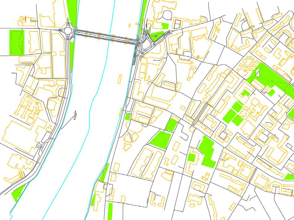
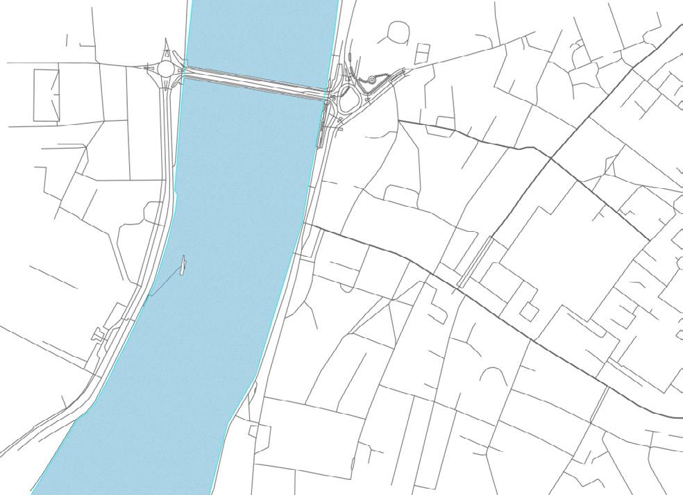
A : Street Network

Hierarchy in roads is observed
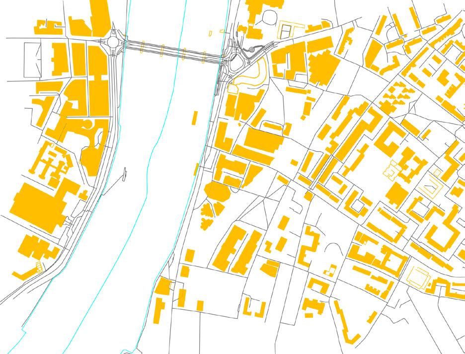
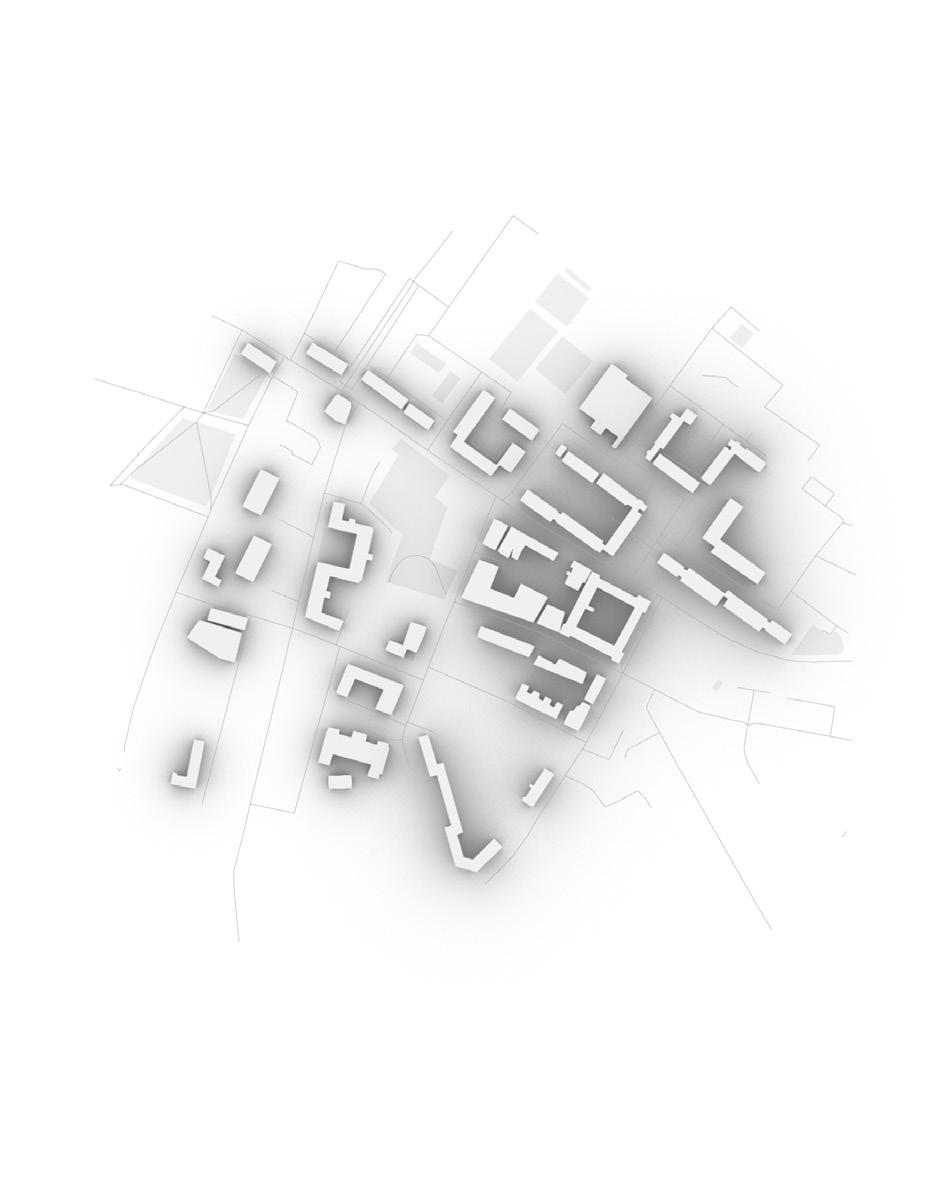
B : Buildings
Densely populated Neighborhoods and clusters
C : Open Spaces
Evenly distributed open spaces amongst the clusters.
D : Waterway
The Thames River : 60 ft wide

E : Amenity Spaces
Evenly distributed amenity spaces within this zone.


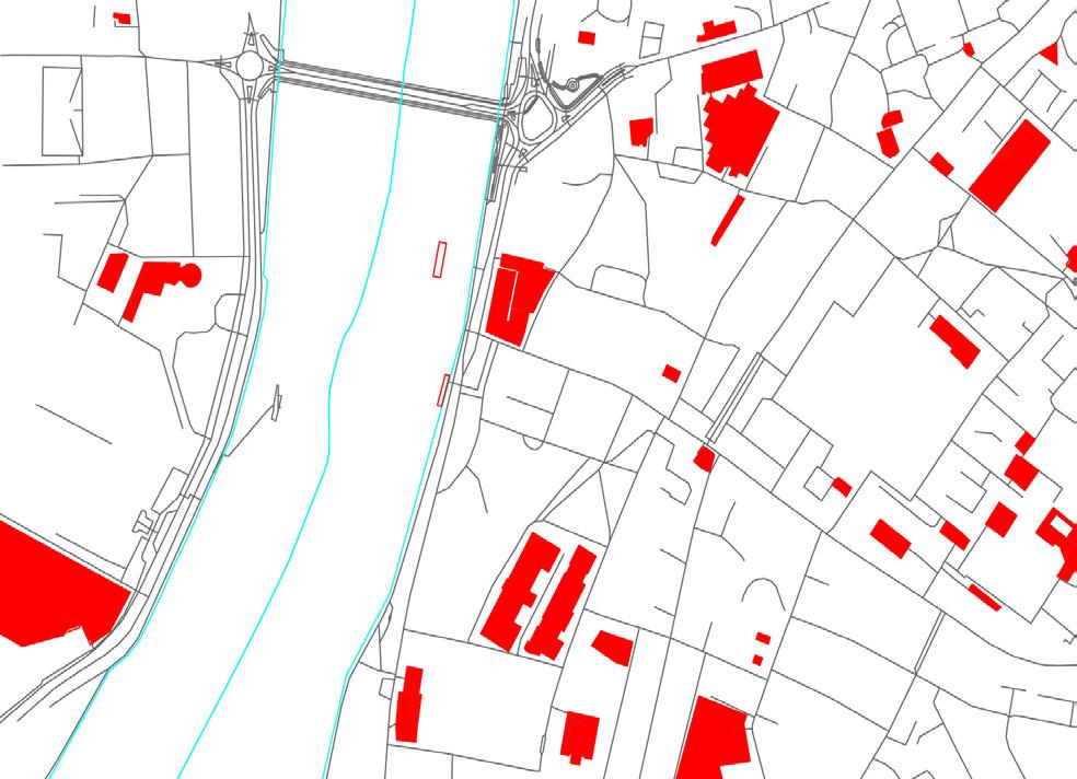
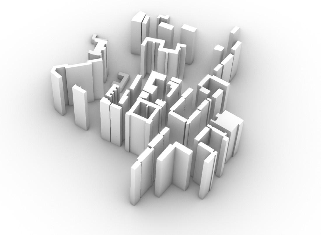
F : 3d Building Extrusions
Allows for extraction of heights of buildings.

5 1.1 ELK MAPS
Location (.osm File)
Open Street Maps
OSM Data Component : Extracts Data for creating layers in Rhino
Cluster : Extracts Points from Elk, the latitude domain and curves to create contours.

3d Buildings from Elk
SRTM Topo: Data File
For Terrain Generation
6
Steps to Run Elk - Step 01 : Load .osm File > Step 02 : .osm File Data Output > Step 03 : Extract Polylines and Bake > Step 04 : Load .srtm topo file
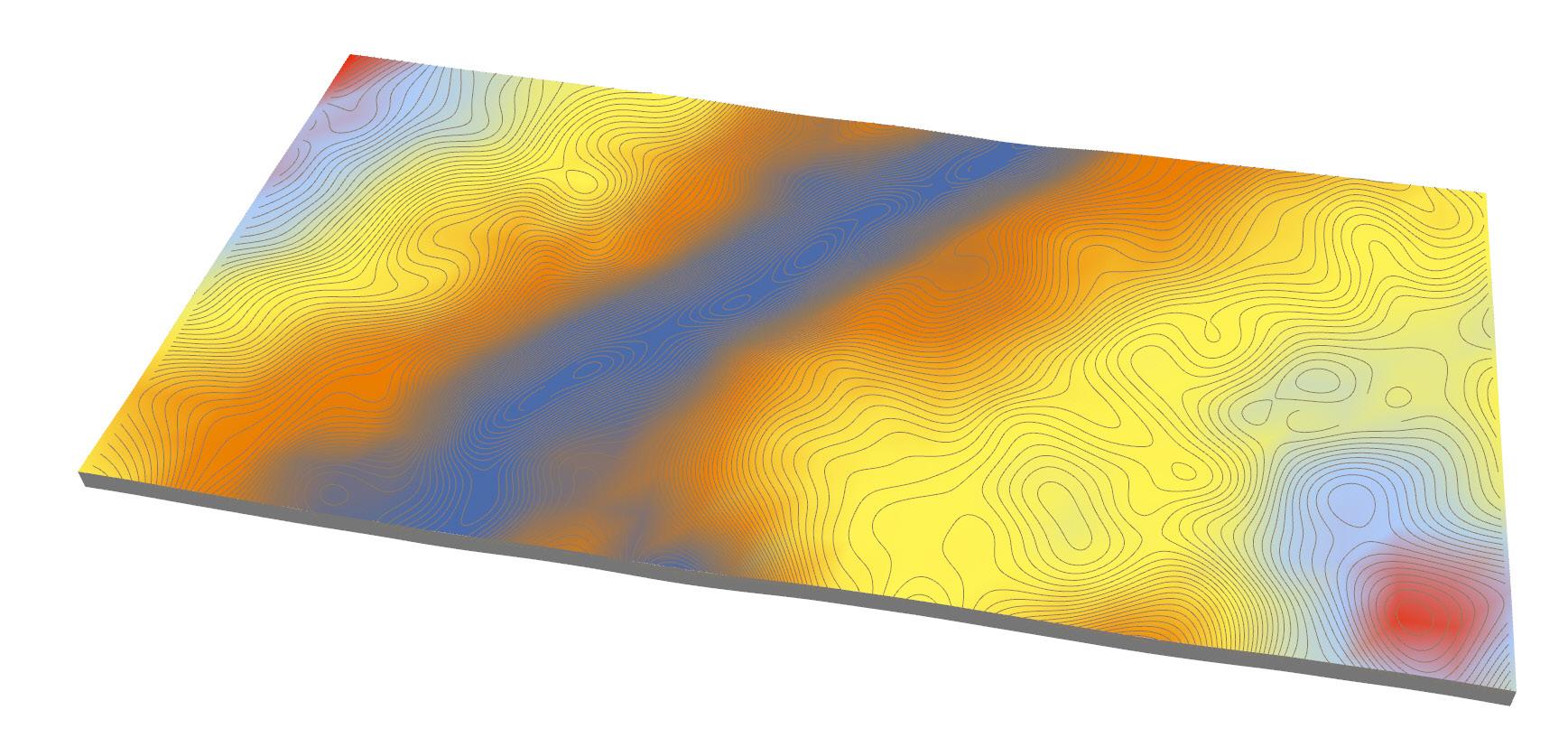
TOPOGRAPHY : TERRAIN GENERATION
Frequency of Contours : Contour Interval: 1 meter
Major Contours : 10 meters


7 1.2 ELK
Steps to Run Elk - Step 01 : Load .osm File > Step 02 : .osm File Data Output > Step 03 : Extract Polylines and Bake > Step 04 : Load .srtm topo file Contour Generation in Plan Achieved Terrain through ELK Cluster for Major and Minor Contours
Major Contours
Minor Contours Legend :
ENVIRONMENTAL ANALYSIS
CHAPTER 02
Plugin : LADYBUG

Use : Environmental Analysis
Data Input Requirements :
EPW format (Weather File)
Source : Ladybug Tools
8
2.1 ladybug : sunpath analysis
Month : January
Time : 12:00 hrs
Month : February
Time : 12:00 hrs
Location : London
Latitude : 51.50 ON
Longitude : 0.1278OW
Month : February
Time : 17:00 hrs
Path of the sun for specified time of the day and month
Location of the sun for specified month along the red loop axis.
Location of the sun for specified time of the day in the specified month.
Legend :
Time of the Year (Path)
Time of the Month (Path)
Location of the Sun


9
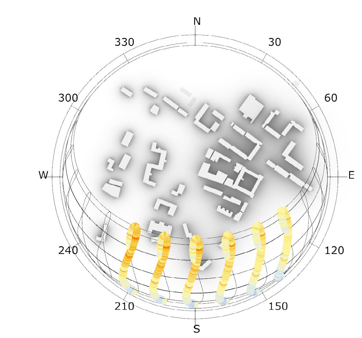
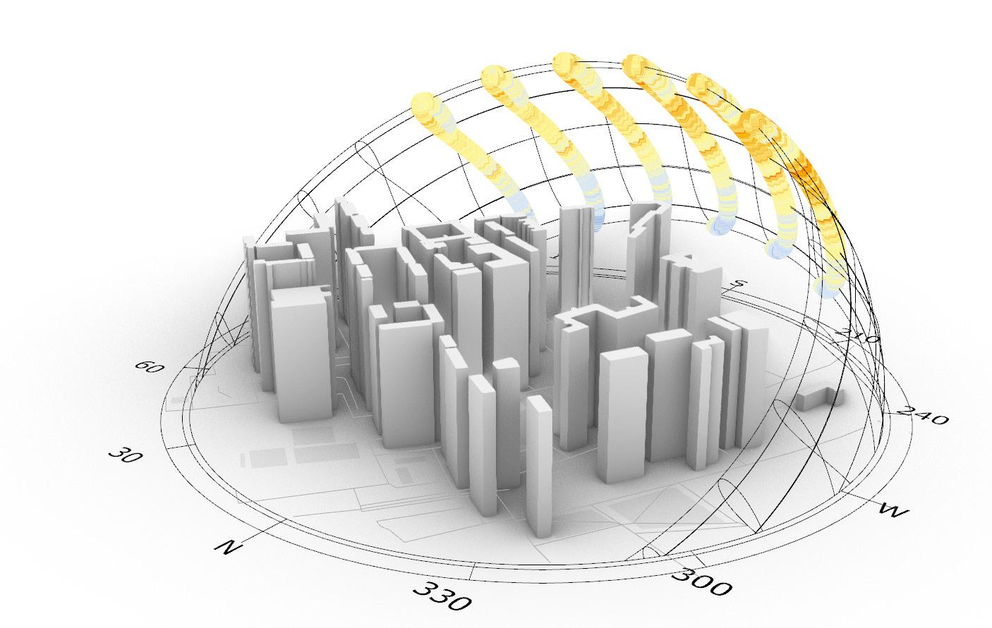
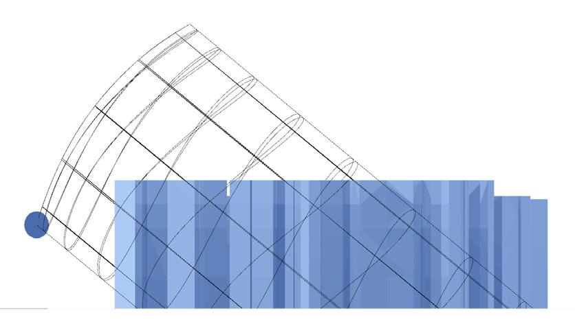
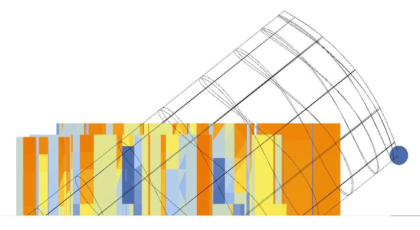
2.1 ladybug : sunpath_Analysis PERIOD
Location : London
Latitude : 51.50 ON
Longitude : 0.1278OW
Hourly Data : Dry Bulb Temperature
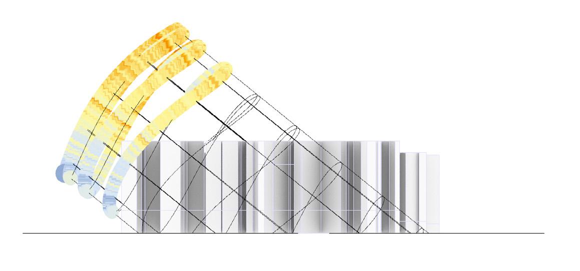
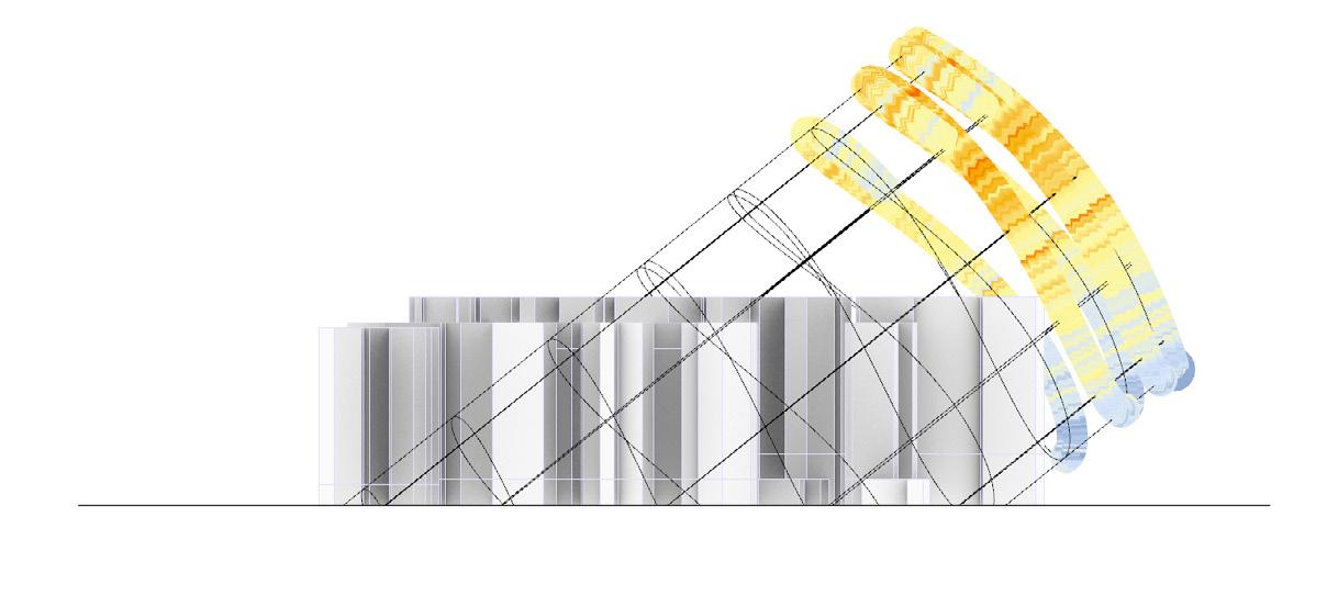
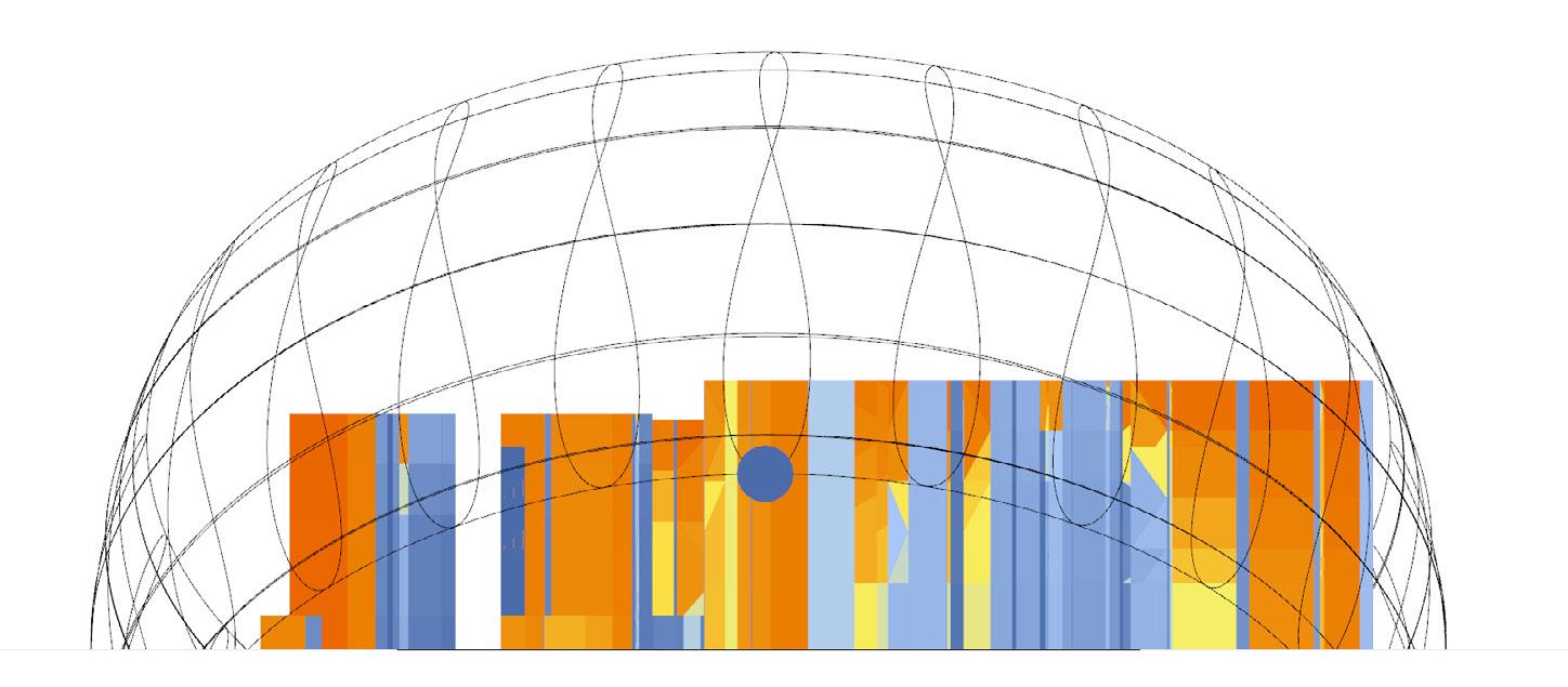
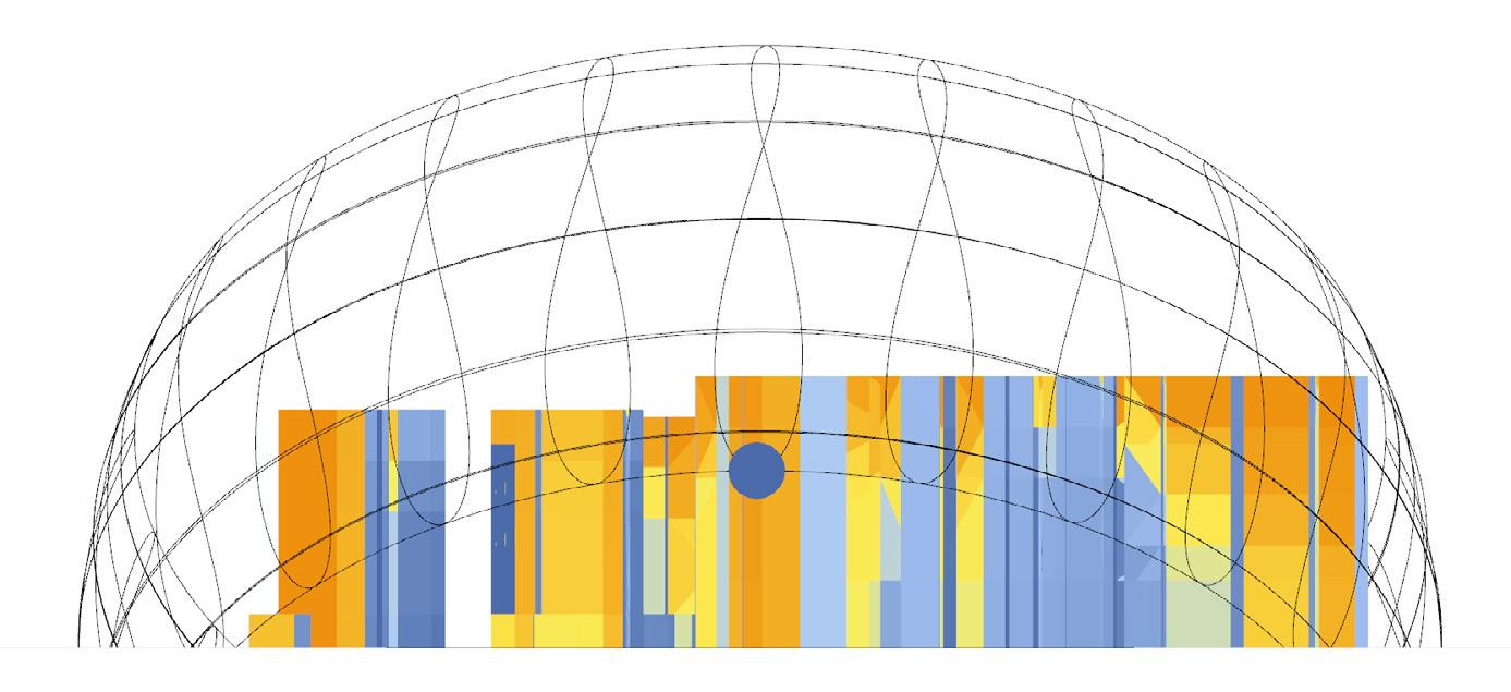
Sun is denoted in different colours which represent temperature as per legend.
Analysis Period :

Months: March to June (3-6)
Day : 23 Hour : 9:00 to 14:00
North Side Elevation
View of the Sunpath Analysis Period


South Side Elevation

10
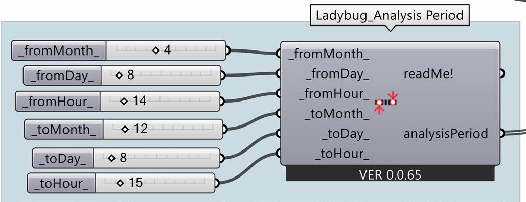
Analysis Period : Annual Hour data of Temperature, humidity, radiation, wind direction etc. can be extracted from the .epw file
Defined Period : By giving Input data of the exact time, day and month , Temperature, humidity, radiation, wind direction etc. can be extracted from the .epw file


11
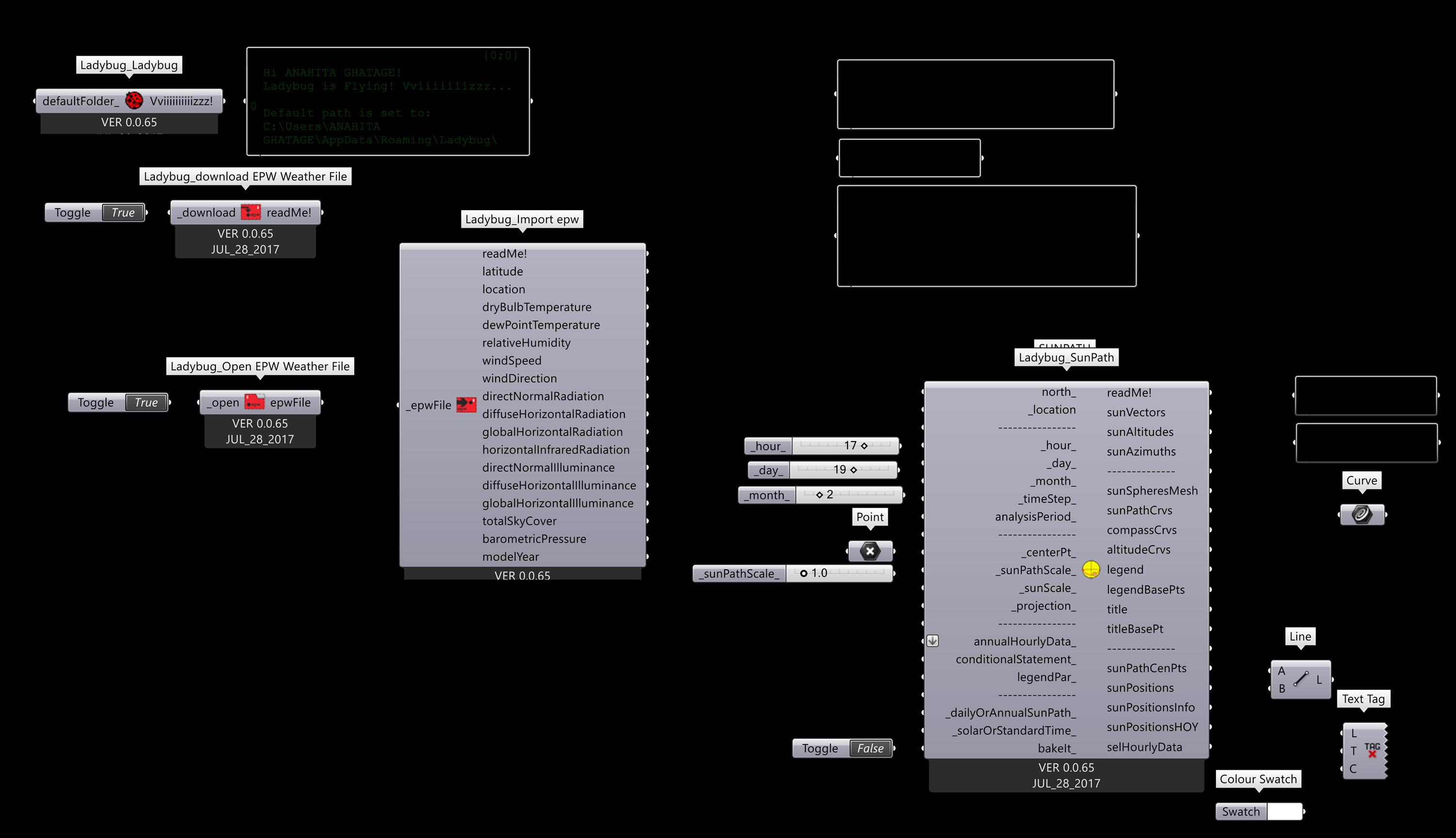
Steps to Run Ladybug - Step 01 : Fly LADYBUG > Step 02 : Download .epw weather file > Step 03 : Open and Import .epw weather file
2.2 ladybug : sHADE AND SHADOW ANALYSIS
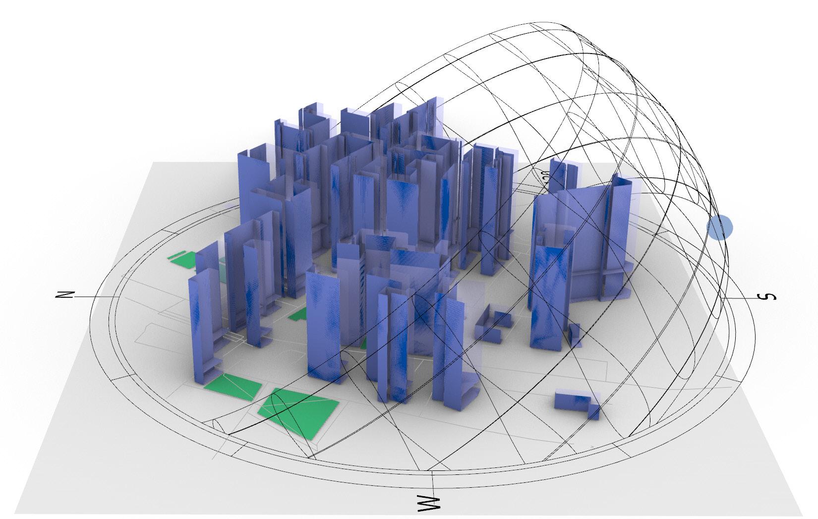
Shade : Darkness created by the shadow
Legend :
Shaded Area
Sunpath Component:

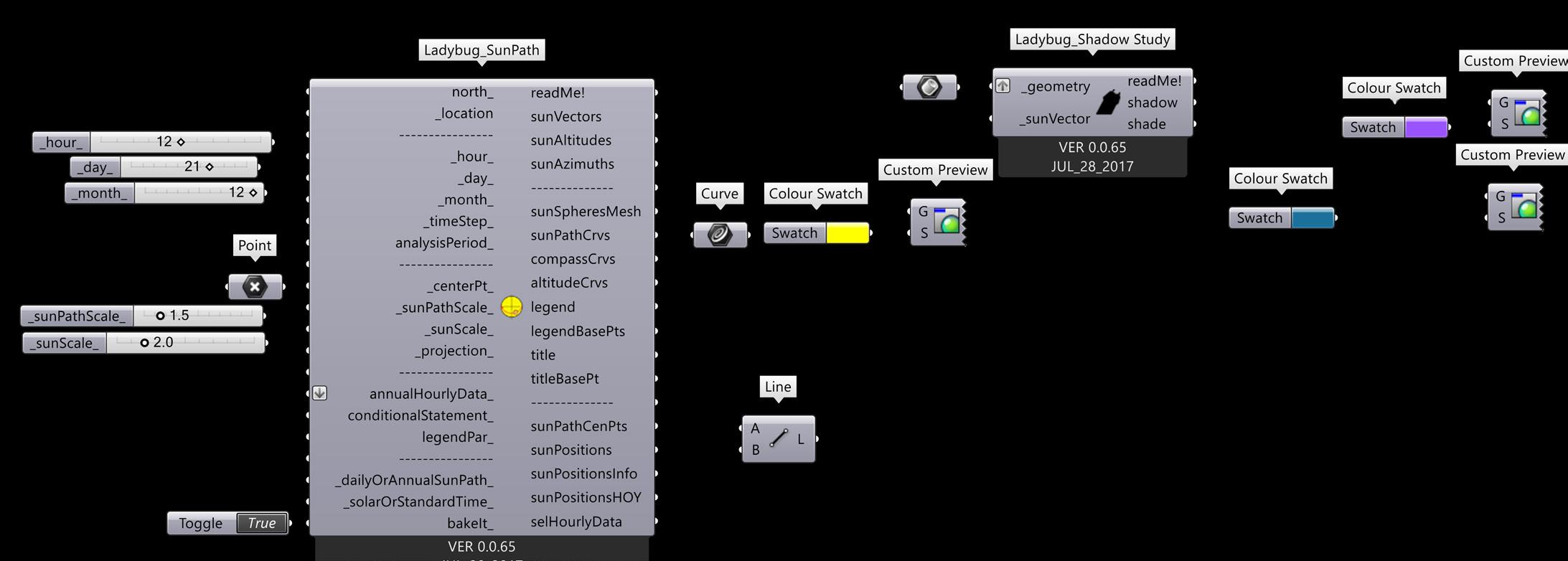
The Shade and Shadow component uses the sun vectors from the sun path component in order to analyse shade and shadows of the buildings.

Location : London
Latitude : 51.50 ON
Longitude : 0.1278OW
Location of the Sun on 19th February, 12:00 hrs
Shade and Shadow Component:
It analyses the amount of shade as well as the shadow cast by the surrounding buildings considering the position of the sun at a given time.
12
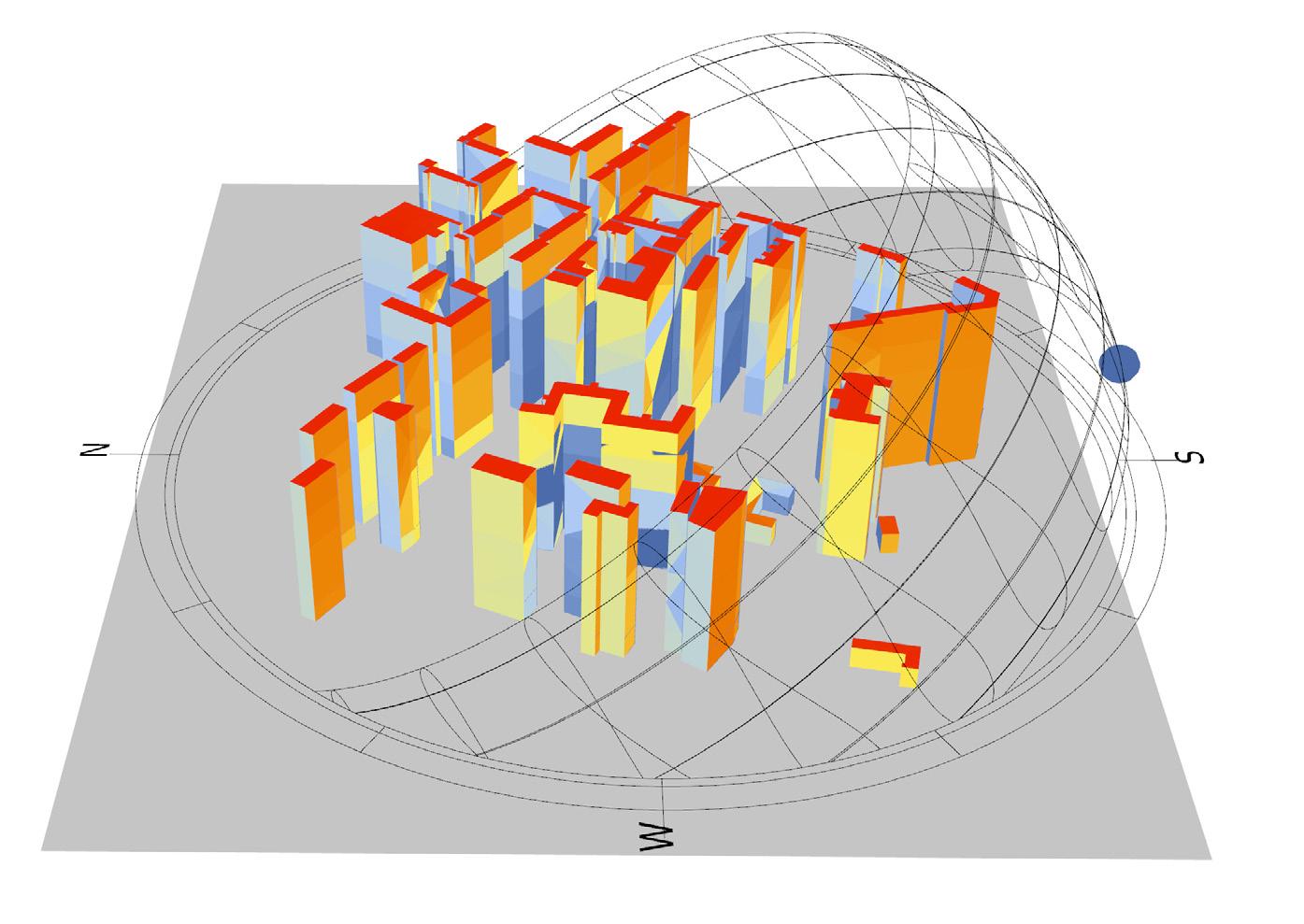
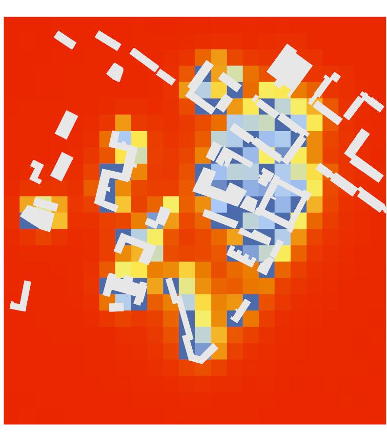
2.3 ladybug : SUNLIGHT HOURS ANALYSIS
Location : London
Latitude : 51.50 ON
Longitude : 0.1278OW
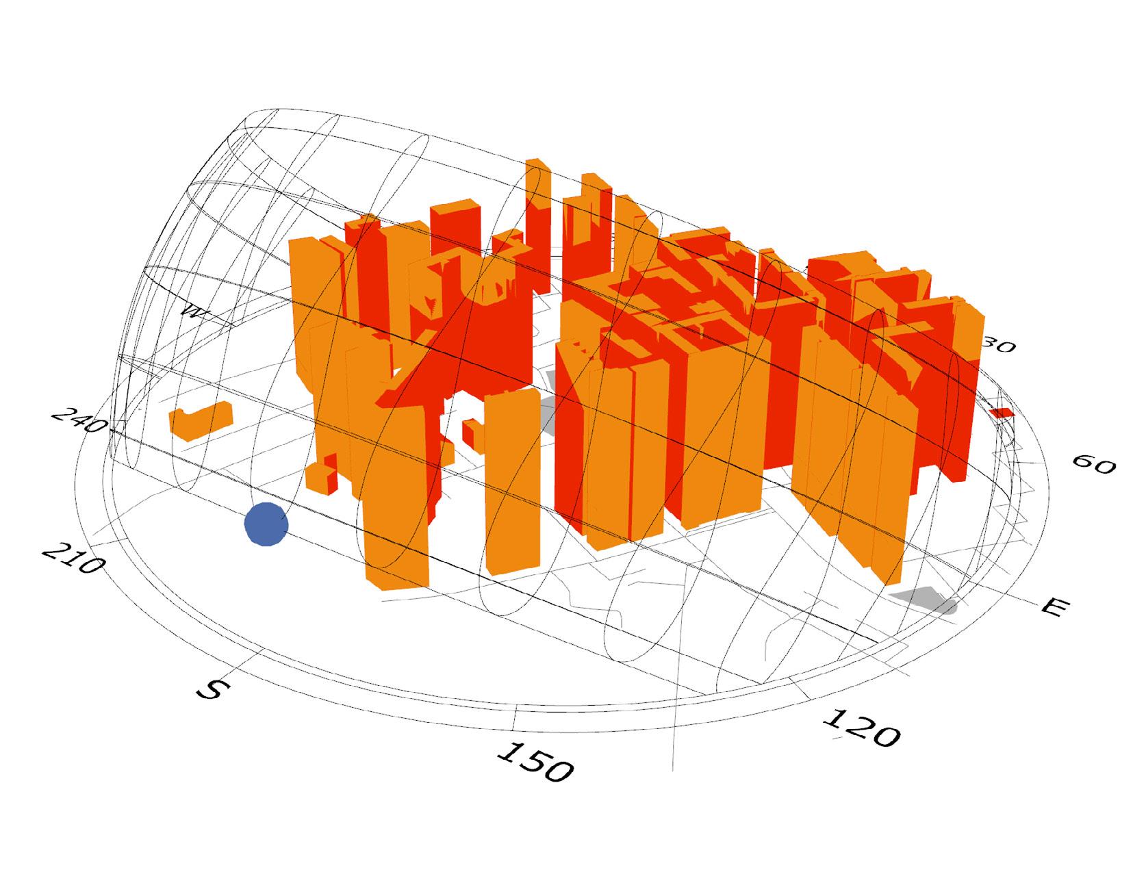
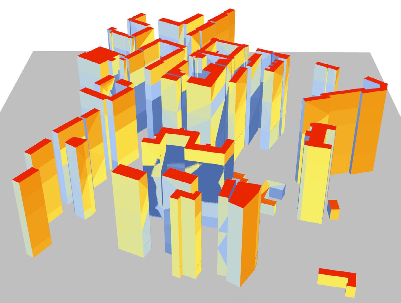
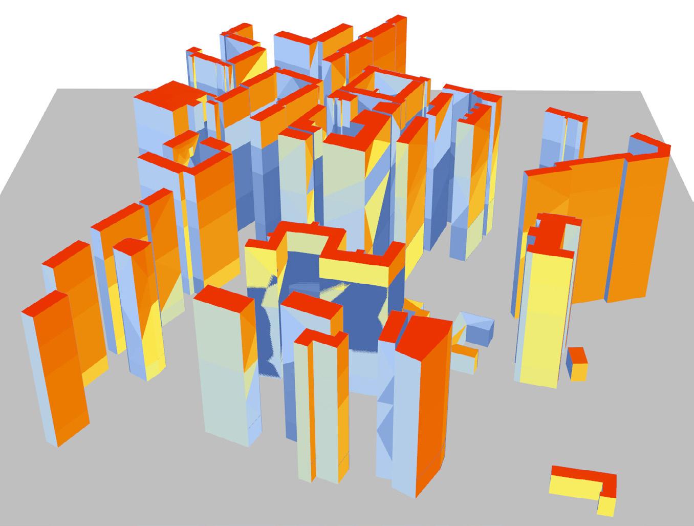
(PLAN) Number of hours the building would receive direct sunight.

Sun Location at 15:00 hrs on 21st January
(PERSPECTIVE) Number of hours the building would receive direct sunight.
LEGEND PARAMETER - The colour goes towards the brighter shade showing the effect of sunlight hours at the specified time of the day.
13
N 30 60 E 120 150 S 210 240 W 300 330 0.00 1.00 2.00 3.00 4.00 5.00 6.00 7.00 8.00 9.00 10.00 Hours N 30 60 E 120 150 S 210 240 W 300 330 0.00 1.00 2.00 3.00 4.00 5.00 6.00 7.00 8.00 9.00 10.00 Hours
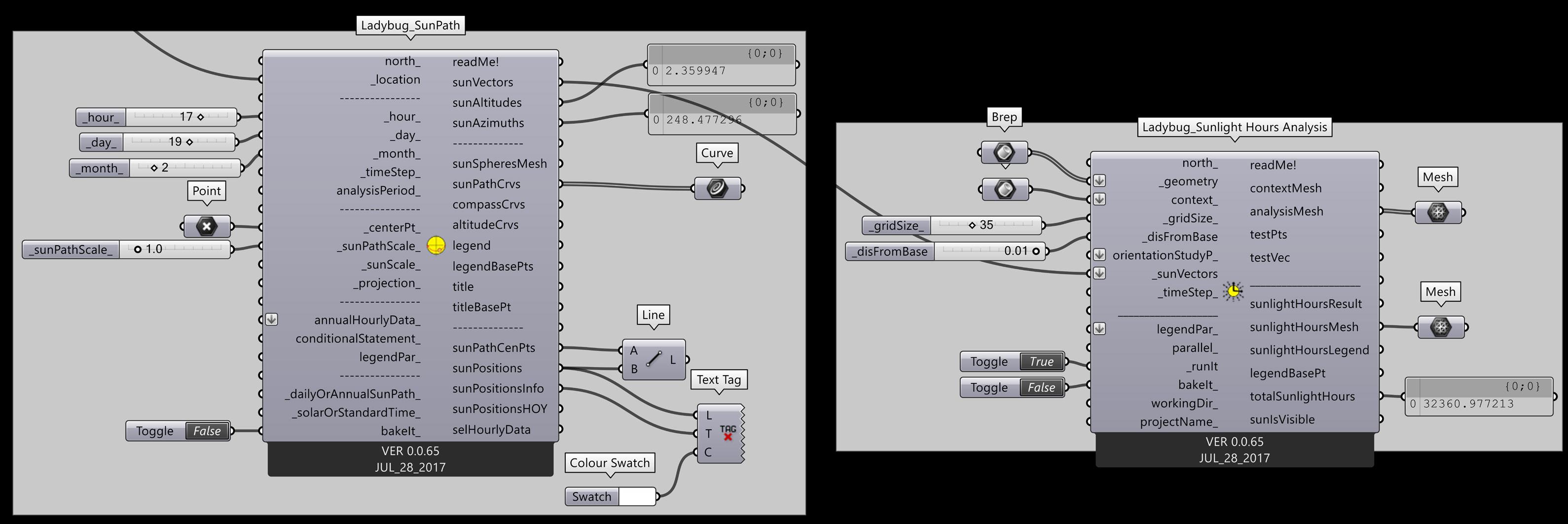
Sunpath Analysis Component : Ladybug uses .epw file for collecting data. The sunpath component’s sun vector output is used by sunlight hour analysis component to generate data.
Sunlight Hours Component: It analyses the direct sunlight received by the geometry at the particular period given and gives an hourly colour legend output.
SUNLIGHT HOUR COMPONENT - The component uses data from the .epw file and the sun vectors from the sunpath analysis to produce sunlight hour analysis data. The input BREP Geometry is the buildings and the ground plane is the CONTEXT.

14
2.4 ladybug : SOLAR RADIATION ANALYSIS
Radiation Analysis on 8h day of April from 14:00 hrs to 15:00 hrs

Ground Plane : 0.07 to 0.71 kWh/m2

Radiation affects the ground plane when the context is the surrounding buildings. The shadow cast by the buildings influences the amount of radiation received by the ground plane.

Location : London
Latitude : 51.50 ON
Longitude : 0.1278OW
Radiation Received by Buildings

North Side Elevation : 0.12 to 0.36 kWh/m2

South Side Elevation : 0.73 to 1.21 kWh/m2

15
Radiation on 15h day of June from 14:00 hrs to 15:00 hrs


Radiation on 15h day of August from 14:00 hrs to 15:00 hrs


Location of the Sun on 15th June from 14:00 hrs to 15 hrs
Location of the Sun on 15h day of August from 14:00 hrs to 15:00 hrs
16
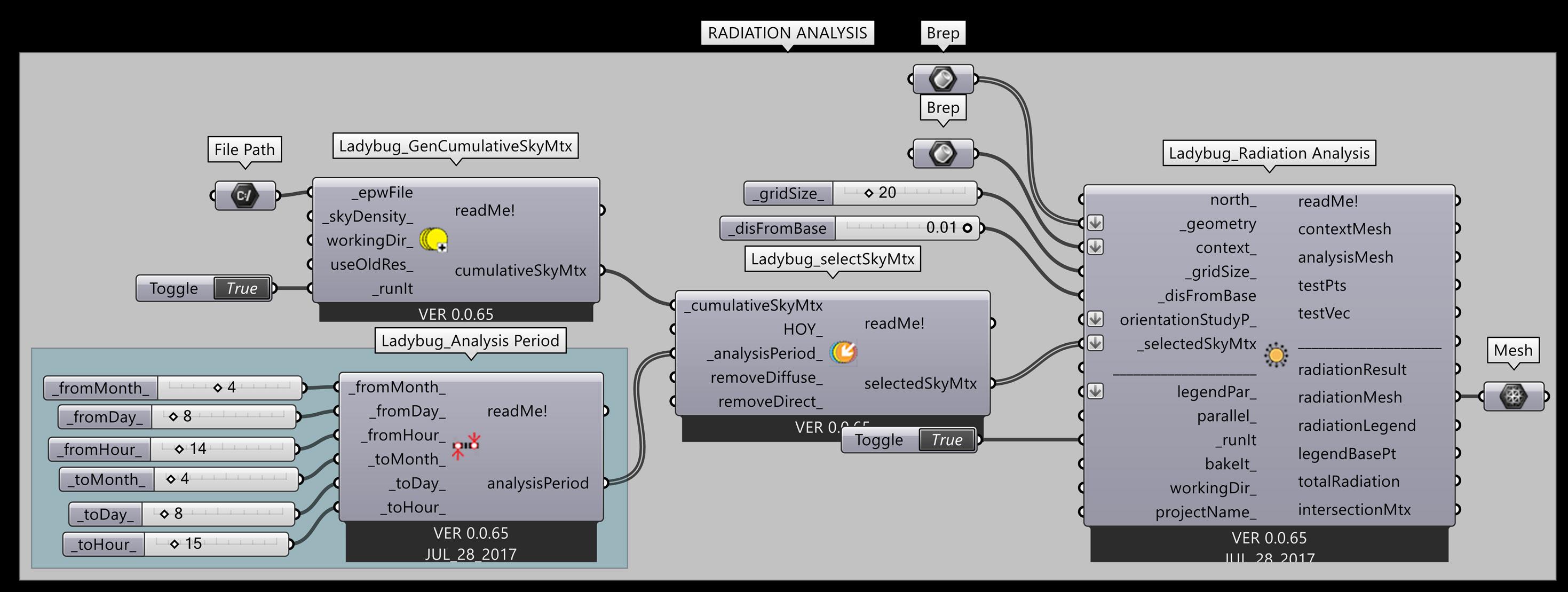
Cumulative Sky Matrix Component: Calculates Sky Radiation for each hour of the year using Radiance’s gendaymtx function.

Select Sky Matrix Component: To select a specific Sky Matrix
RADIATION ANALYSIS COMPONENT - The component uses data from the .epw file and the CUMULATIVE SKY MATRIX component in order to produce the data for radiation analysis. The context for analysis could be the buildings or the ground plane.
17
2.5 ladybug : RADIATION ROSE
Location : London
Latitude : 51.50 ON
Longitude : 0.1278OW
Diffuse Radiation
Total Solar Radiation
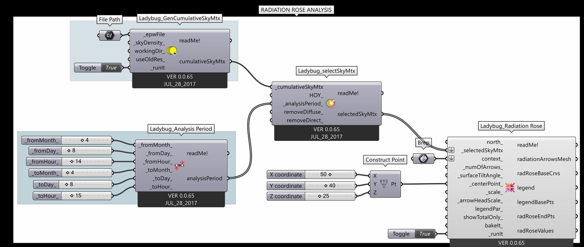
Ladybug Radiation Rose Component :

It uses select Sky Matrix for the data. It generates a chart showing radiation (kwH/M2) data at a particular direction. The arrow shows the direction of the radiation and the length of the arrow shows the time period.
The colour denotes the intensity of the radiation.
18
0.00 0.07 0.13 0.20 0.27 0.33 0.40 0.47 0.53 0.60 0.67 kWh/m2 350 N 10 20 30 40 50 60 70 80 E 100 110 120 130 140 150 160 170 S 190 200 210 220 230 240 250 260 W 280 290 300 310 320 330 340 350 N 10 170 S 190 200 210 220 230 240 250 260 W 280 290 300 310 320 330 340 0.00 0.07 0.13 0.20 0.27 0.33 0.40 0.47 0.53 0.60 0.67 kWh/m2 350 N 10 20 30 40 50 60 70 80 E 100 110 120 130 140 150 160 170 S 190 200 210 220 230 240 250 260 W 280 290 300 310 320 330 340 350 N 10 170 S 190 200 210 220 230 240 250 260 W 280 290 300 310 320 330 340
8 April 14:00 hrs - 8 April 15:00 hrs 0.00 0.07 0.13 0.20 0.27 0.33 0.40 0.47 0.53 0.60 0.67 kWh/m2 350 N 10 20 30 40 50 60 70 80 E 100 110 120 130 140 150 160 170 S 190 200 210 220 230 240 250 260 W 280 290 300 310 320 330 340 0.00 0.05 0.10 0.15 0.20 0.24 0.29 0.34 0.39 0.44 0.49 kWh/m2 0.00 0.07 0.13 0.20 0.27 0.33 0.40 0.47 0.53 0.60 0.67 kWh/m2 350 N 10 20 30 40 50 60 70 80 E 100 110 120 130 140 150 160 170 S 190 200 210 220 230 240 250 260 W 280 290 300 310 320 330 340 0.00 0.05 0.10 0.15 0.20 0.24 0.29 0.34 0.39 0.44 0.49 kWh/m2
April 14:00 hrs - 8 April 15:00 hrs
8
View Point :
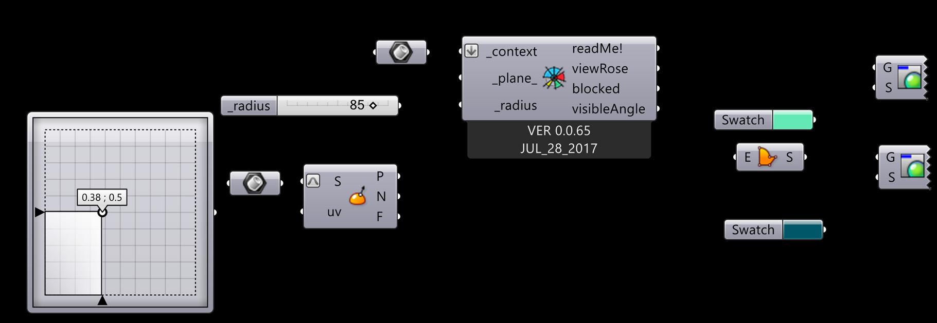
The Plane is the point from which the view is visualized. This can be moved using the evaluate surface component.
Location : London
Latitude : 51.50 ON
Longitude : 0.1278OW
Radius:


The radius of the view rose is the area that is too be considered for blocked views and visibility.
View Rose Component : It uses the context as the buildings and shows which elements block the view and which views are clear.


19
2.6 ladybug : VIEW ROSE
72% of Blocked Views
28% of Blocked Views
47% of Blocked Views
Blocked View Legend : Visibility View Point
NNE N
NE
ENE
E
ESE
SE
m/s 10.60 NNW NW WNW W WSW SW SSW S SSE
m/s 10.60 9.54 8.48 7.42 6.36 5.30 4.24 3.18 2.12 1.06 0.00
Location : London
Latitude : 51.50 ON
Longitude : 0.1278OW
Wind Rose Component : Ladybug Wind Rose uses the .epw file to extract the wind speed and direction. This generates a pie chart showing wind speed (m/s) data at a particular direction. In this case, WEST & SOUTH WEST direction.
Colour : The colour denotes the speed (m/s)
Wind-Rose London Wea Ctr St James Park_ENG_GBR 8
Wind-Rose London Wea Ctr St James Park_ENG_GBR 8
APR 14:00 - 8 DEC 15:00 Hourly Data: Wind Speed
APR 14:00 - 8 DEC 15:00 Hourly Data: Wind Speed
(m/s) Calm for 0.02% of the time = 1 hours. Each closed polyline shows frequency of 0.1%. = 4 hours.

20
NNW NW WNW W WSW SW SSW S SSE SE ESE E ENE NE NNE N
2.7 ladybug : WIND ROSE
(m/s) Calm for 0.02% of the time = 1 hours. Each closed polyline shows frequency of 0.1%. = 4 hours. 9.54 8.48 7.42 6.36 5.30 4.24 3.18 2.12 1.06 0.00
Wind Rose Diagram
Wedges : The percentage of time the wind came from that particular direction.
2.8 ladybug : PSYCHROMETRIC CHART

Comfort Polygons are different for different activities.
Cleaning : 35 kj/kg to 55kj/kg Dancing : 25 kj/kg to 45 kj/kg
Activity: House Cleaning Activity: Dancing
Location : London
Latitude : 51.50 ON
Longitude : 0.1278OW
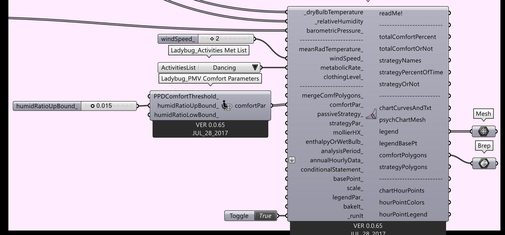
Psychrometric Chart:
A psychrometric chart is a graphical representation of the psychrometric processes of air. Psychrometric processes include physical and thermodynamic properties such as dry bulb temperature, wet bulb temperature, humidity, enthalpy, and air density.
PSYCHROMETRIC CHART COMPONENT - The component uses data from the .epw file of the relative humidity, dry bulb temperature and the barometric pressure to derive comfort polygons for the specified activity.
21 Hours 133.00<= 119.70 106.40 93.10 79.80 66.50 53.20 39.90 26.60 13.30 <=0.00 110 kJ/kg 100 kJ/kg 90 kJ/kg 80 kJ/kg 70 kJ/kg 60 kJ/kg 50 kJ/kg 40 kJ/kg 30 kJ/kg 20 kJ/kg 10 kJ/kg 0 kJ/kg -10 kJ/kg 90% 80% 70% 60% 50% 40% 30% 20% 10% 0.03 0.025 0.02 0.015 0.01 0.005 50 45 40 35 30 25 20 15 10 5 0 -5 -10 -15 -20 Hours 133.00<= 119.70 106.40 93.10 79.80 66.50 53.20 39.90 26.60 13.30 <=0.00 110 kJ/kg 100 kJ/kg 90 kJ/kg 80 kJ/kg 70 kJ/kg 60 kJ/kg 50 kJ/kg 40 kJ/kg 30 kJ/kg 20 kJ/kg 10 kJ/kg 0 kJ/kg -10 kJ/kg 90% 80% 70% 60% 50% 40% 30% 20% 10% 0.03 0.025 0.02 0.015 0.01 0.005 50 45 40 35 30 25 20 15 10 5 0 -5 -10 -15 -20 Hours 133.00<= 119.70 106.40 93.10 79.80 66.50 53.20 39.90 26.60 60 kJ/kg 50 kJ/kg 40 kJ/kg 30 kJ/kg 20 kJ/kg 10 kJ/kg 0 kJ/kg -10 kJ/kg 20% 10% 0.015 0.01 0.005
Operative Temperature Humidity Ratio Humidity Ratio Operative Temperature Hours 133.00<= 119.70 106.40 93.10 79.80 66.50 53.20 39.90 26.60 13.30 <=0.00 70 kJ/kg 60 kJ/kg kJ/kg 20% 10% 0.02 0.015 0.01 0.005 50 45 40 35 30 25 20 110 kJ/kg Hours 133.00<= 119.70 106.40 93.10 79.80 66.50 53.20 39.90 26.60 13.30 <=0.00 70 kJ/kg 60 kJ/kg 50 kJ/kg 40 kJ/kg 30 kJ/kg 20 kJ/kg 10 kJ/kg 0 kJ/kg -10 kJ/kg 20% 10% 0.02 0.015 0.01 0.005 50 45 40 35 30 25 20 15 10 5 0 -5 -10 -15 -20
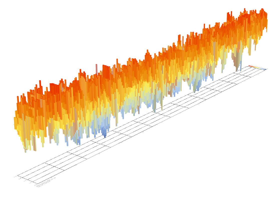
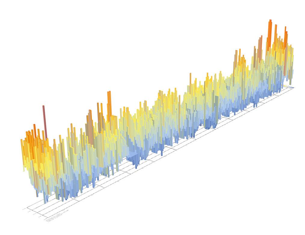
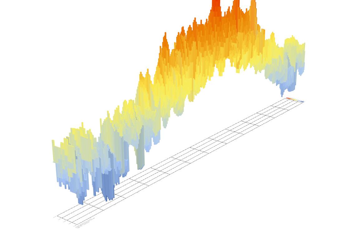
2.9 ladybug : ANNUAL BAR CHARTS
Relative Humidity % - Hourly
Dry Bulb Temperature C - Hourly
Wind Speed m/s - Hourly
Relative Humidity

Dry Bulb Temperature


Wind Speed Chart


22
Jan Feb Mar Apr May Jun Jul Aug Sep Oct Nov Dec Jan Feb Mar Apr May Jun Jul Aug Sep Oct Nov Dec Jan Feb Mar Apr May Jun Jul Aug Sep Oct Nov Dec
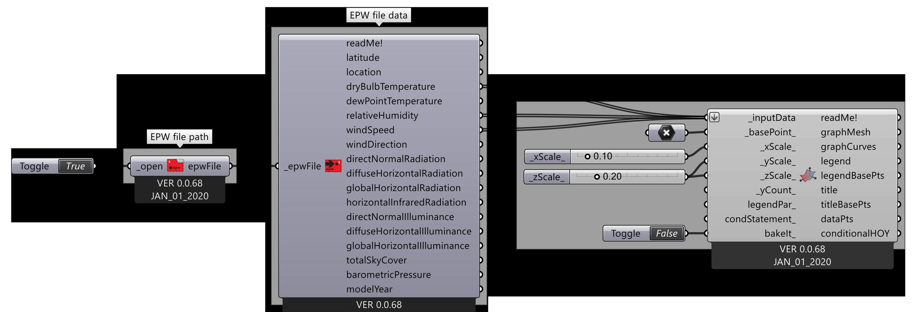
Ladybug EPW file Data :
It uses the .epw file for the data. Annual charts can be generated for Wind speed, Radiation, Dry bulb Temperature, Relative humidity, etc.
Ladybug 3d Chart :
It uses the .epw file for the data. Required climate data should be given as input. This will generate a 3d chart for the annual climatic data. A conditional statement can be mentioned, which will remove the data that does not fit the conditions.

23
CHAPTER 03
Plugin : SLOPE ANALYSIS
Use : Slope Degree & Elevation
Buildable and Non - Buildable Slopes
24
DA1905_2019-20
TERRAIN
3.1 SLOPE ELEVATION

Highest Elevation
Recessed Elevation

River Bed
Elevated Land Area
High Elevated Land Area
Legend :
Low points
High Points
Inference:
The site has a 12 meter gradient throughout its surface. The slope in towards the river on either side of it.
Lowest Point Highest Point
25
3.2 SLOPE DEGREE
Highest Degree Slope Value
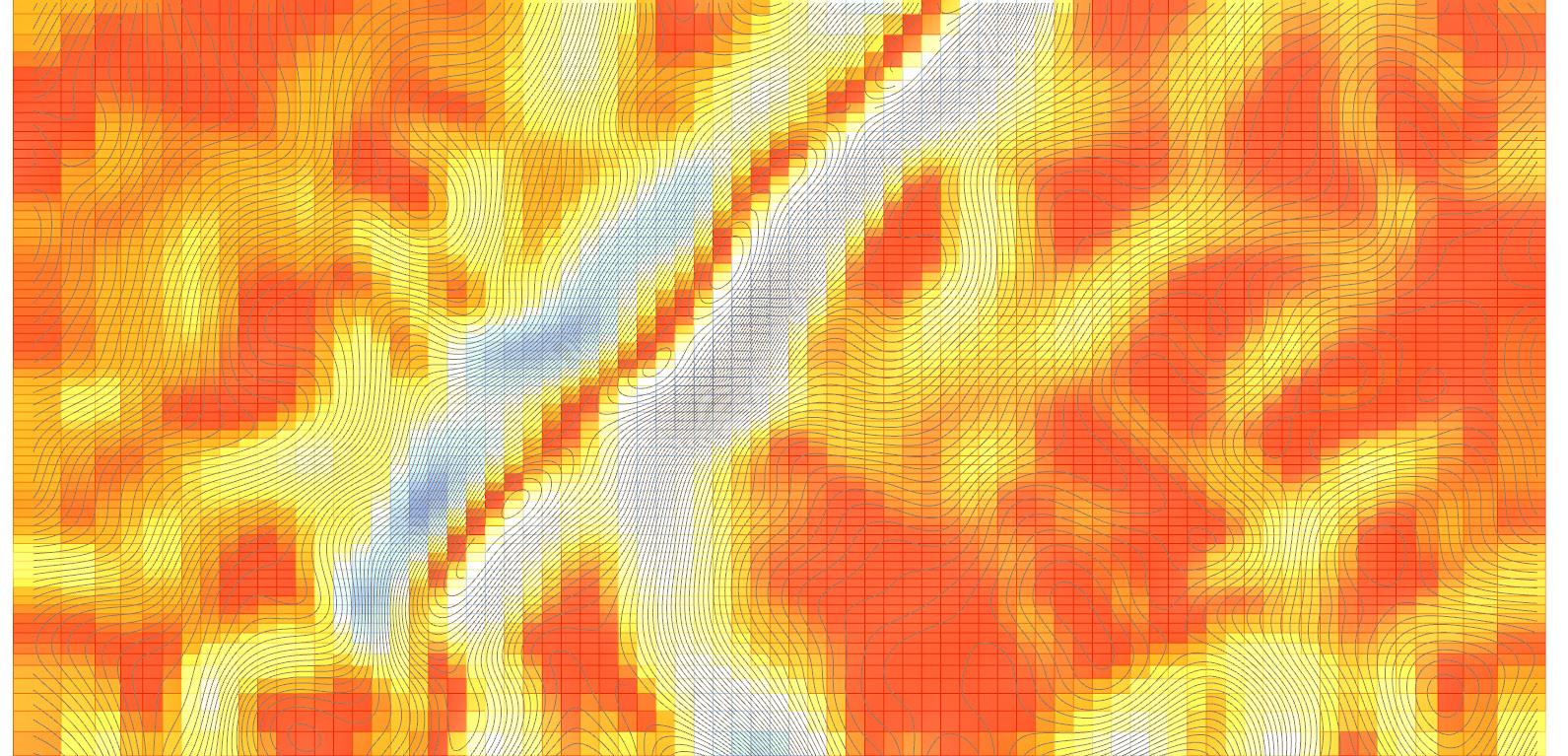
Slope identifies the steepest downhill slope for a location on a surface.

The Evaluate Surface command takes an input surface raster and calculates an output raster containing the slope at each cell. The lower the slope value, the flatter the terrain; the higher the slope value, the steeper the terrain. The output slope raster can be calculated as percent slope or degree of slope.

Inference: The site has slope degree of 0.18 to 0.77 units.
Lowest Degree Slope Value

Highest Degree
Lowest Degree
26
CHAPTER 04
Plugin : SPACE SYNTAX
Use : Space Zoning & Networks


27
NETWORKS
4.1 SPACE syntax theory
Representations of space
Spatial elements are represented through their geometric forms and how people experience them. They can be geometrically derived (for example, point, axial line, segment, convex space and isovist) or functionally defined (for example, rooms in building).
Analysis of spatial relations
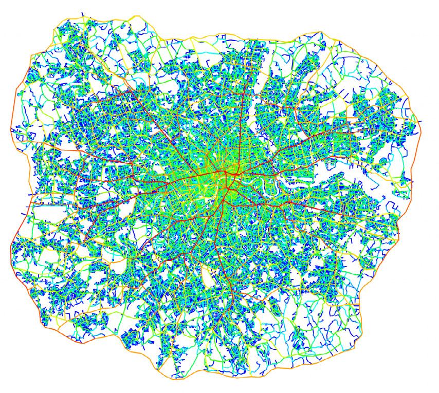
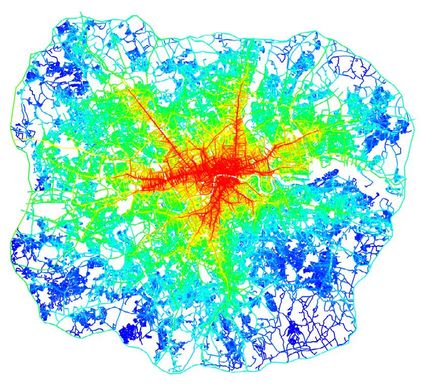
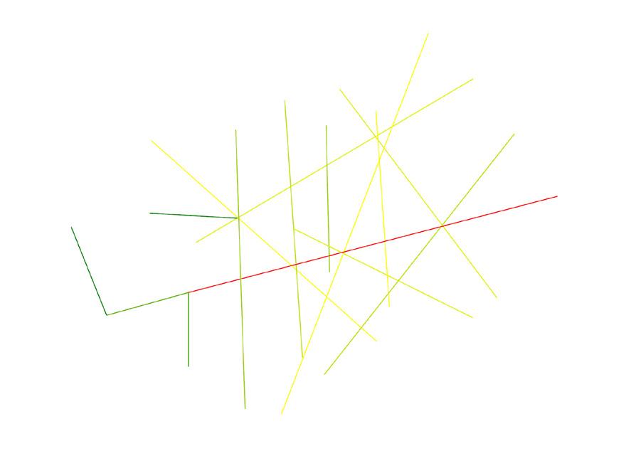
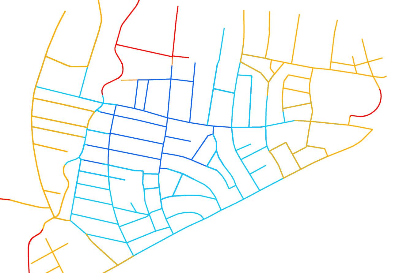
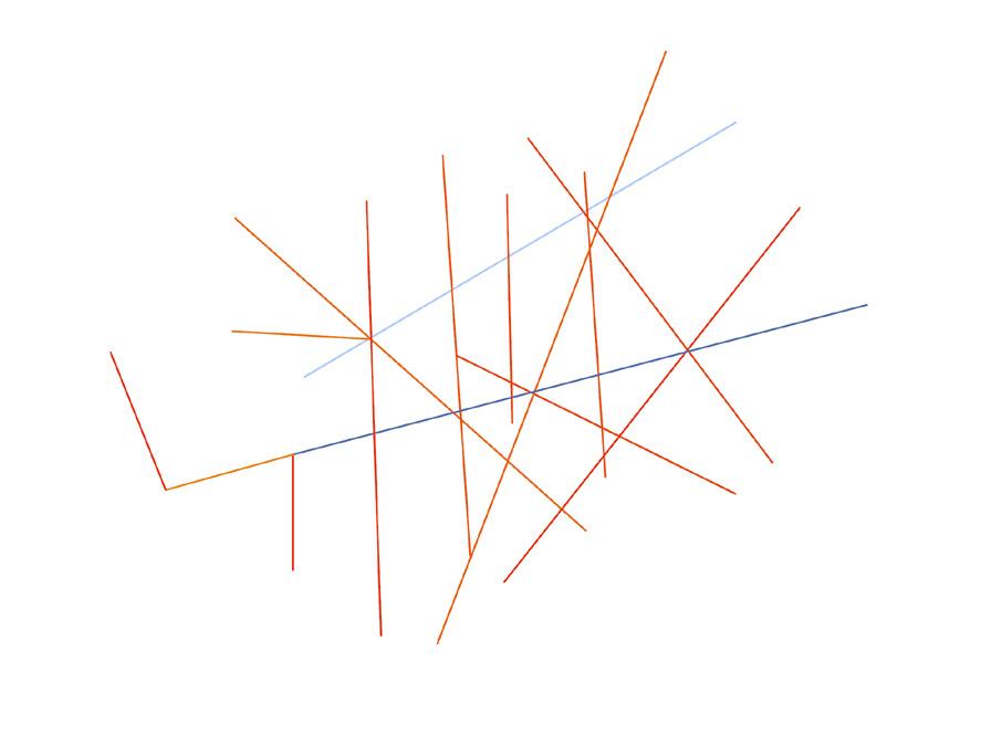
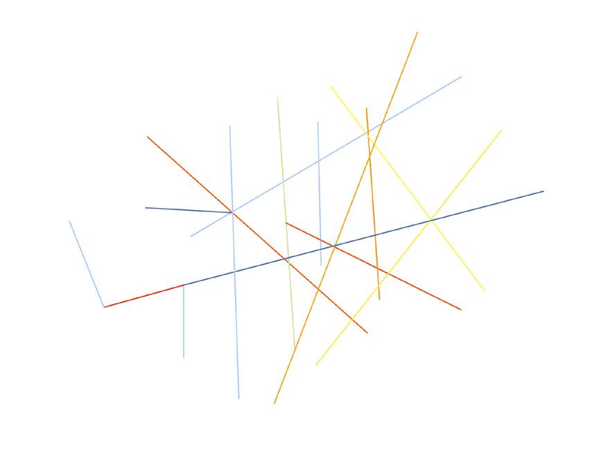
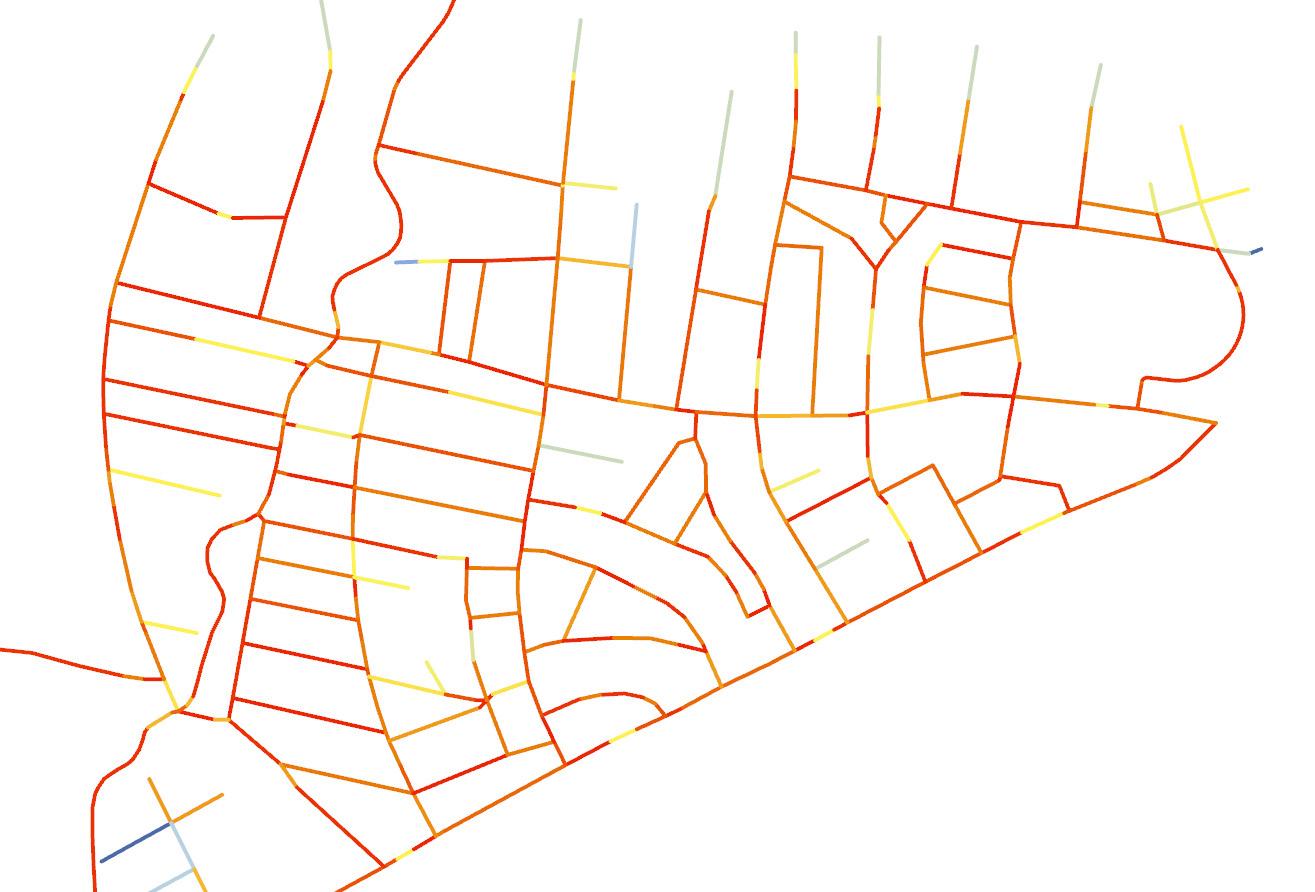
Relationships between spatial elements result from their configuration. These relationships can be objectively analysed using various measures, included among which are integration(see figure A) and choice (see figure B ). These two measures reflect the two fundamental elements in human movement: firstly, the selection of a destination, and secondly, the selection of a route. One measures the ease of access (integration) and the other measures the passing flow (choice).
Interpretive models
Spatial models are developed to analyse, describe, explain and forecast different kinds of spatial and socio-economic phenomena. Practically,models are created to investigate empirical phenomena such as urban movement, urban crime, and centrality as a process as well as for general processes such as spatial intelligibility.

Reference : http://otp.spacesyntax.net/

28
A. Space Syntax Integration Pattern of Greater London
A. Space Syntax Choice Pattern of Greater London
Representations of space
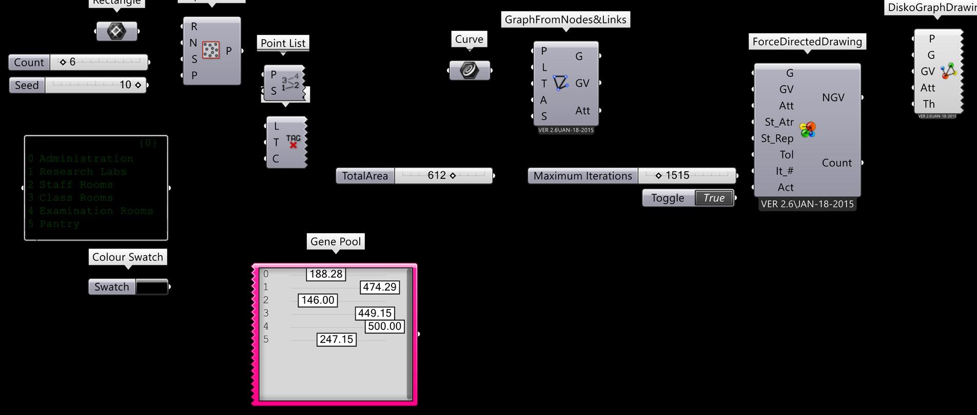
The Plugin requires data regarding :

The list of spaces that it needs to create (populate rectangle with points)
The areas of these spaces (gene pool)
The areas that need to be connected to each other
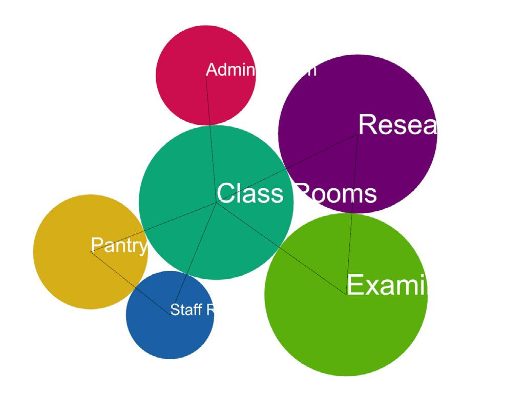
The Disko Graph Drawing Component and the Force Directed Drawing Component tries to establish a relationship based on the data provided and gives various iterations for zoning options based on the connections and areas as constraints to generate the drawing.
Connections Between the Spaces

29 4.2 SPACE
Research Labs
Administration Pantry Staffroom Examination Room
SYNTAX
Classrooms
Disko Graph Drawing Output Iteration
4.3 INTEGRATION

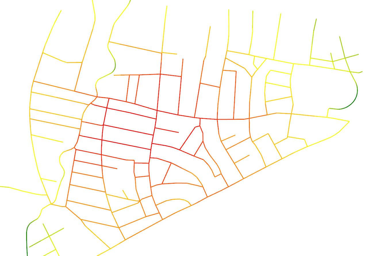
Integration Pattern of an area in London


The higher the integration value the more communal space is likely to be, the lower the value, the more private the space is likely to be.
Legend : Semi-Public Space
More Communal Space
Private Space
30
Diagram explaining Integration
Indicates how often a node happens to be the shortest path between other spaces.


Least Likely Used Legend : Moderately Used
Most Likely Used
31 4.4 BETWEENESS
/ CHOICE
Diagram explaining Betweeness
Betweeness Pattern of an area in London
Diagram explaining Centrality
Control : A local dynamic measure describing what degree of choice does each space represent for its immidiate neighbors to move to.


Centrality Pattern of an area in London

Least Likely
Legend : Moderately
Most Likely
32 4.5 CENTRALITY
AGENT BASED MODELLING
CHAPTER 05
Plugin : Physarealm | Quelea | Zebra

Use : Agent Based Modelling (ABM)
Theory Base : Slime Mould, Patterns
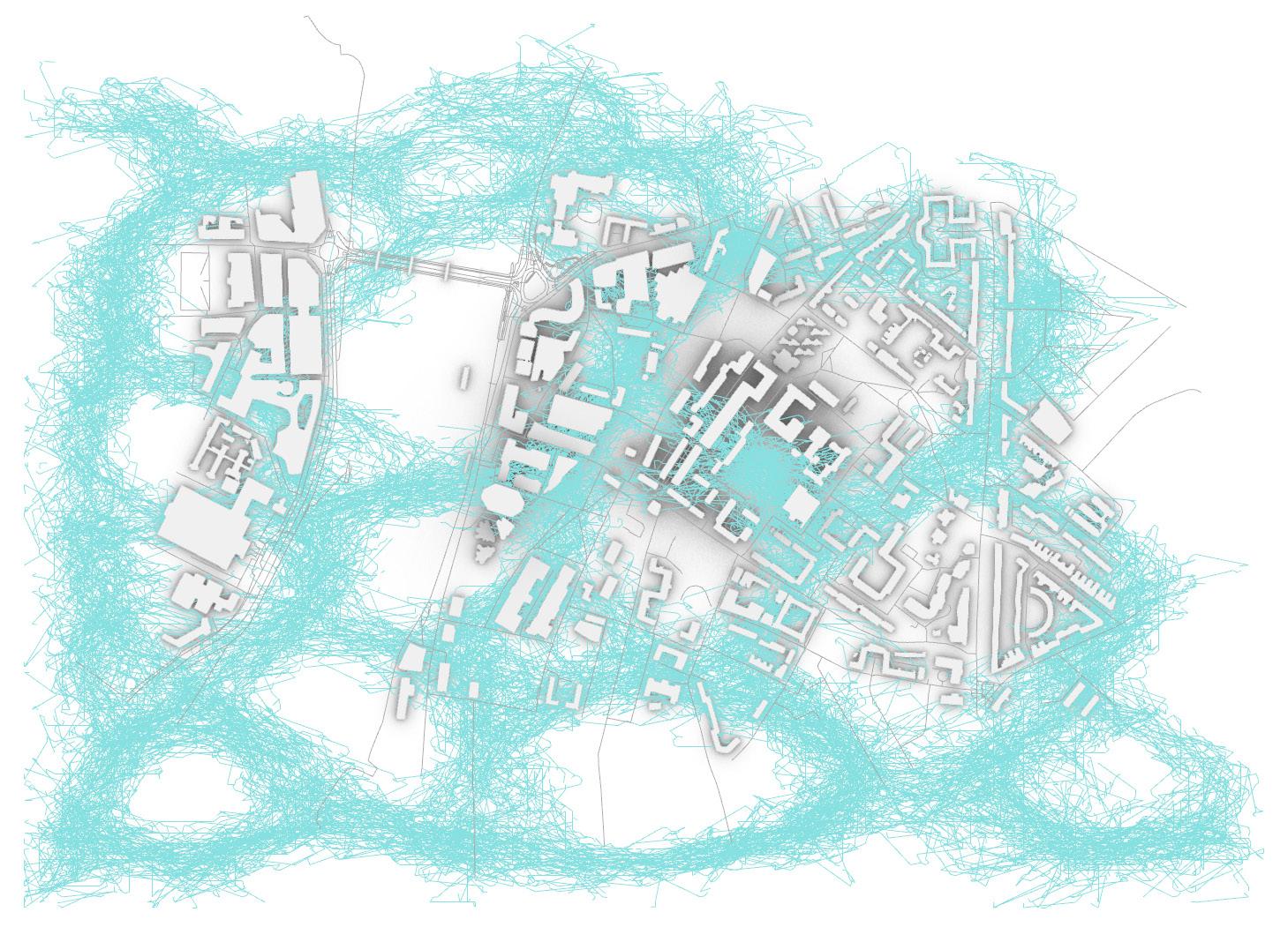
Optimises to give the most efficient solution based on Crowd Behaviour Simulation , Shortest Path

33

34 5.1 AGENT
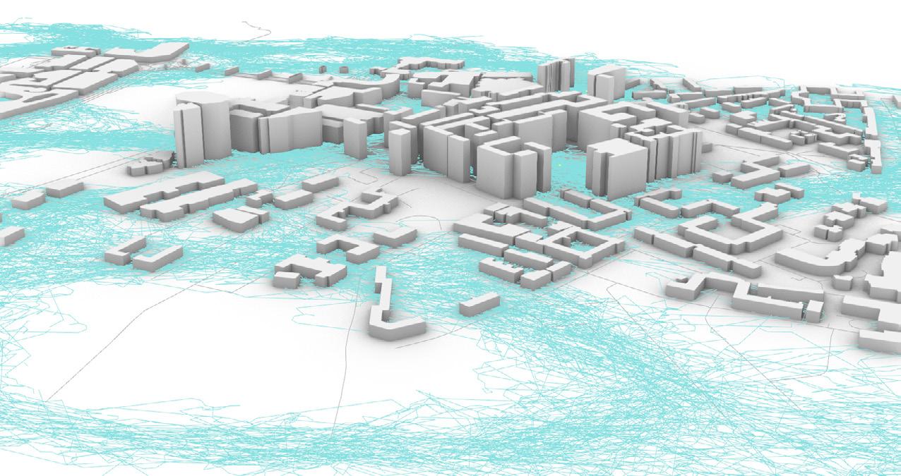
Food Source Emitter Path taken by Physarealm
BASED MODELLING : PHYSAREALM
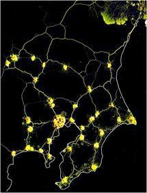
Slime Mould : A group of Japanese researchers has shown that P. polycephalum can find the shortest route connecting two food sources when placed in a maze with two oatmeal flakes. In a 2010 paper, P. pocephalum (Slime Mould) created a network similar to the existing Tokyo train system when oatmeal flakes were dispersed to represent towns on a map of the Tokyo area. Inspiration from this natural phenomenon has raised questions regarding how we can mimic and emulate it to find solutions to path planning. Architects and urban designers often face spatial planning problems, such as finding effective paths between points of interest.

Surface Environment : Boundary Condition, where, agents run on a uv space.

Birth Death Settings: Parameter for Birth and Death condition of Agents.
Physarealm : Shortest Path
Population Interconnect: Connects pair of agents locations below a certain distance.
Physarealm Component: Agent Based Modelling
Population Trail: It gives the trails of each agent.

35
5.2 AGENT BASED MODELLING : QUELEA

Applications of Flocking : In Cologne, Germany, two biologists from the University of Leeds demonstrated a flock-like behavior in humans. The group of people exhibited a very similar behavioral pattern to that of a flock, where if 5% of the flock would change direction the others would follow suit. When one person was designated as a predator and everyone else was to avoid him, the flock behaved very much like a school of fish. Flocking has also been considered as a means of controlling the behavior of Unmanned Air Vehicles (UAVs).Flocking is a common technology in screensavers, and has found its use in animation. Flocking has been used in many films to generate crowds which move more realistically. It has also been used for visualizing information and for optimization tasks.
Separation Alignment Cohesion
Rule Sets of Flocking Behavioural System
Construct Agent : Constructs the settings for an agent
Box Emitter : Box environment for the agent

Quelea as Flocking Agents : Imitating the flocking of the quelea bird (always in groups).
Deconstruct Particle : Deconstucts a particle to expose its fields, i.e, Position, Velocity, Acceleration
Contain Force : Applies a force to keep agents away from the Environment Boundary

36
CHAPTER 06
Plugin : GALAPAGOS
Use : Single Objective Optimisation
Theory Base : Evolutionary Algorithm
Optimises to give the most efficient solution based on number constraints.

37
ALGORITHM
EVOLUTIONARY
6.0 Theory of evolutionary algorithm
INDIVIDUAL A
BREEDING
INDIVIDUAL B
PHENOME
GROWTH
BREEDING
Gene Expression
Body Plan
Cross-over Recombination
MUTATIONS
EMERGENCE OF POPULATION
SURVIVING PHENOMES
Alterations in Gene Sequence
Natural Selection
38
6.1 evolutionary algorithm - a
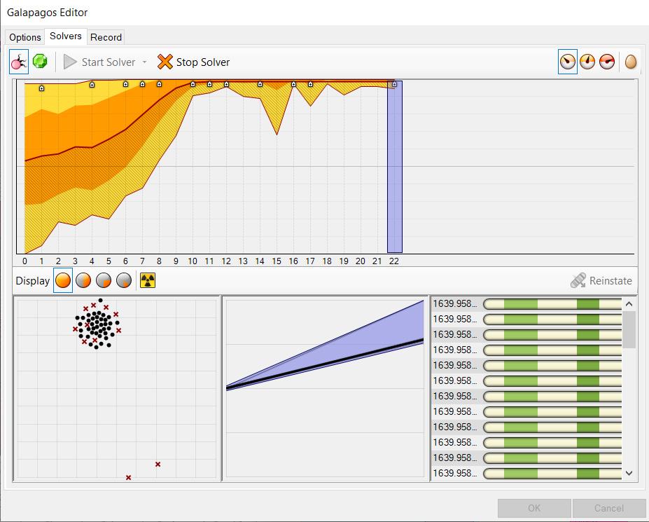
Galapagos Genetic Input : Galapagos can operate on anynumber of Slider objects. It requires certain sliders to be assigned to the Galapagos object for them to become part of the ‘Genome’. It is best to limit the slider range as much as possible, as this reduces the size of the search space.

Galapagos Fitness Input : Galapagos requires a single parameter which provides a fitness value. When Galapagos runs, it will attempt to maximize or minimize this fitness. Fitness parameters need not be number parameters. Any data type that can be converted into a number.
3D
Optimisation
Optimisation Graph

Genomes
Iterations Genrated
39
6.2 evolutionary algorithm - b


3D Optimisation_ Bounding Box

Optimizing for Minimum Volume of the Bounding Box
3D Optimisation Using Bounding Box

Number of Floors
Optimization for Floor Space Index of a Building
FAR Optimization
Site Curve to Evaluate Along
Number of Floors
Minimum Difference
Site Line to Evaluate
Galapagos Evolutionary Solver
Maximum Floor Area : Minimum Number of Floors Given : Site Constraint
40
CHAPTER 07
Plugin : OCTOPUS
Use : Multi Objective Optimisation
Theory Base : Evolutionary Algorithm
Optimises to give iterations based on number constraints.

41
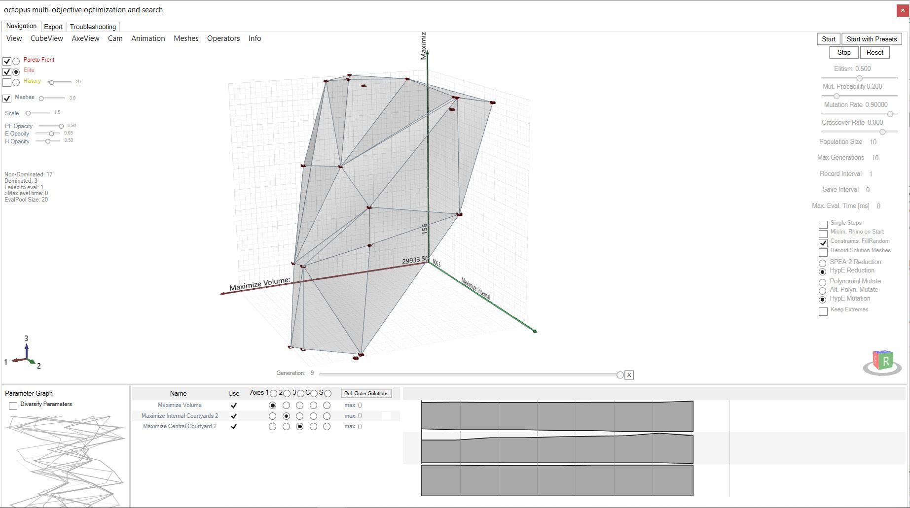
7.1 OCTOPUS - COURTYARD OPTIMISATION
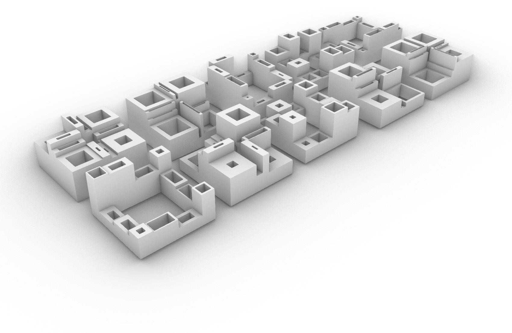
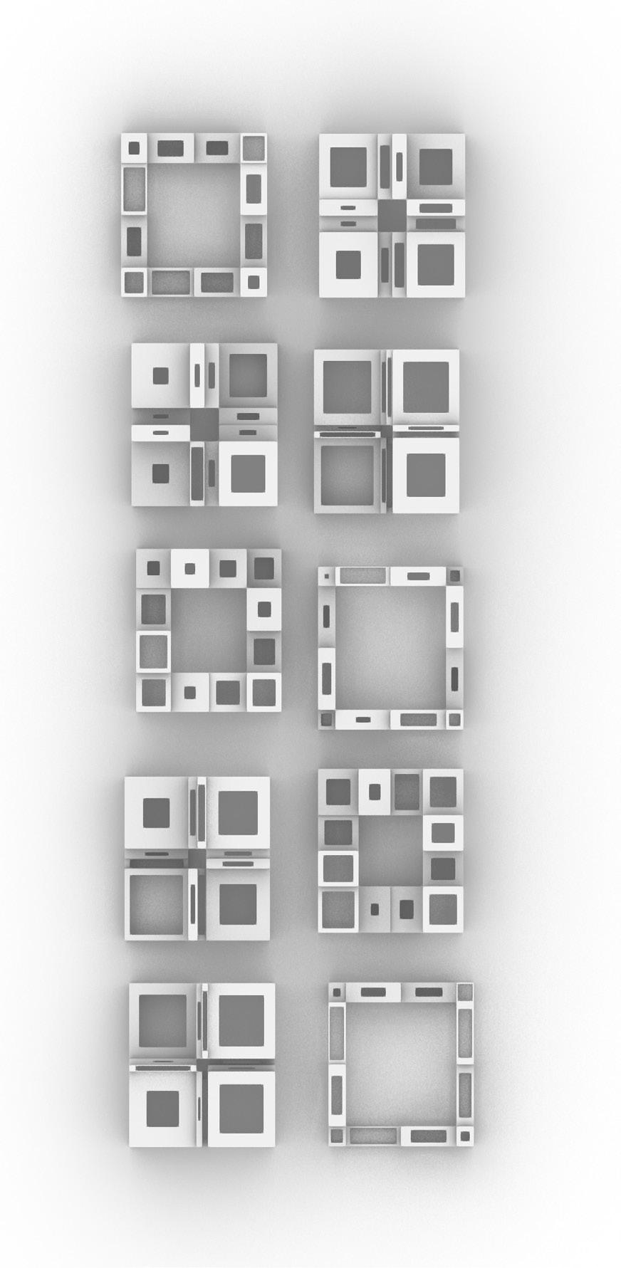
Optimised Courtyard Iterations for Maximum Volume : Maximum Internal Courtyards : Maximum Central Courtyard

Axis : Criterias
Maximize Volume
Maximize Internal Courtyard
Delaunay Mesh Iterations

Maximize Central Courtyard
Results
Optimised Courtyard Iterations for Maximum Volume :
Maximum Internal Courtyards : Maximum Central Courtyard

42
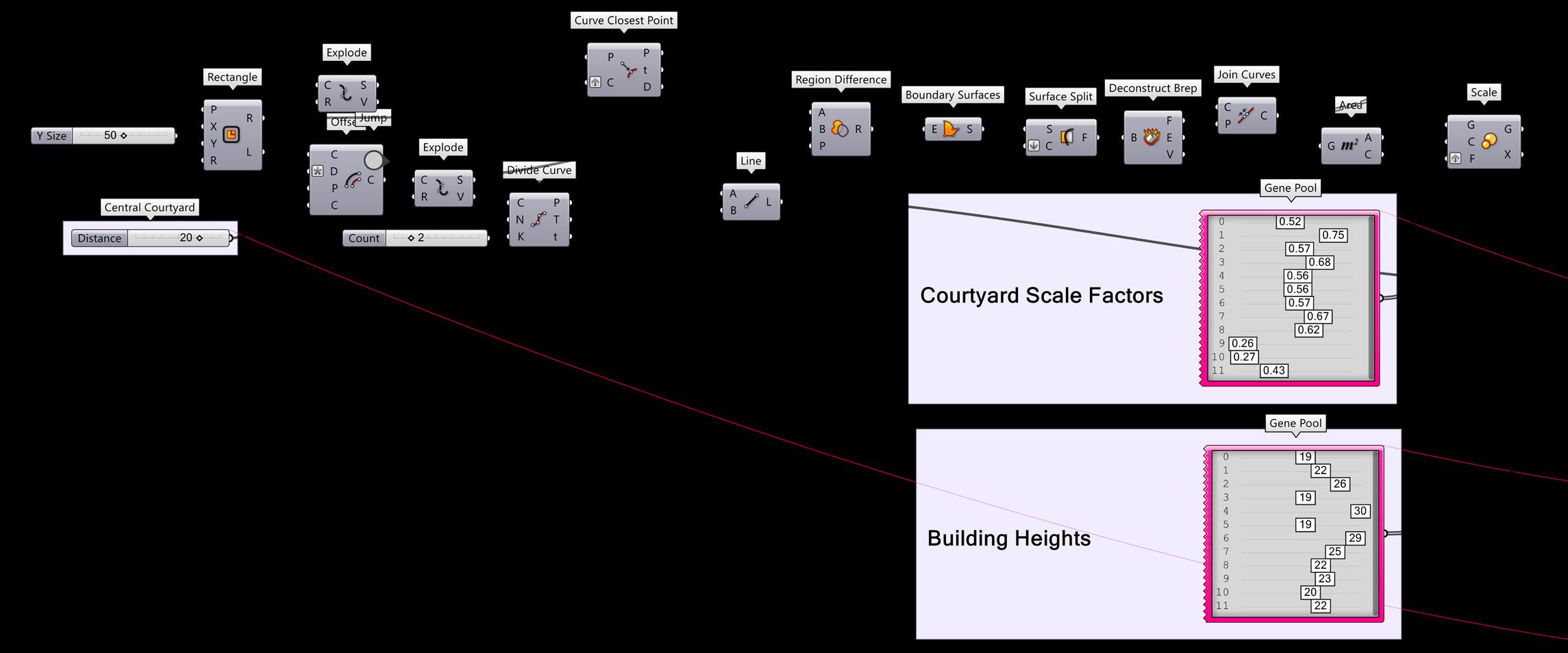
- BUILDING THE ALGORITHM
Offset Rectangle: Used to create smaller courtyards
Region Difference : Used to create the Central Courtyard
Octopus was originally made for Multi-Objective Evolutionary Optimization. It allows the search for many goals at once, producing a range of optimized trade-off solutions between the extremes of each goal. It is used and works similar to David Rutten’s Galapagos, but introduces the Pareto-Principle for Multiple Goals.


G : Genome (Inputs for Octopus to solve)
O : Multi-objective Optimisation Solving
Obtain Number containers for the Maximum Possible Volume, Maximum Internal Courtyards and Maximum Central Courtyard. Use subtraction between the maximum values and changing values. Obtain these values in a number container.
Now, Octopus will optimise between the values and keep them the difference the lowest.
Courtyard Scale Factors : Create a gene pool with and randomize the courtyard values. This goes as criteria 01 for the octopus solver. i.e. Maximum Area of Courtyards.
Building Heights Factors : Create a gene pool with and randomize the building heights. This goes as criteria 02 for the octopus solver. i.e. Maximum Heights of Buildings, i.e Maximum Volume.

43
7.1 OCTOPUS
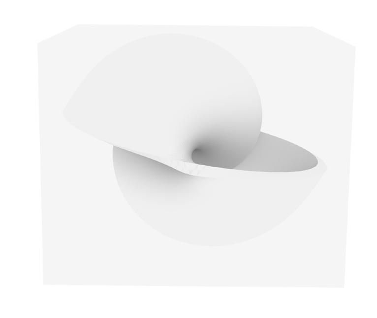
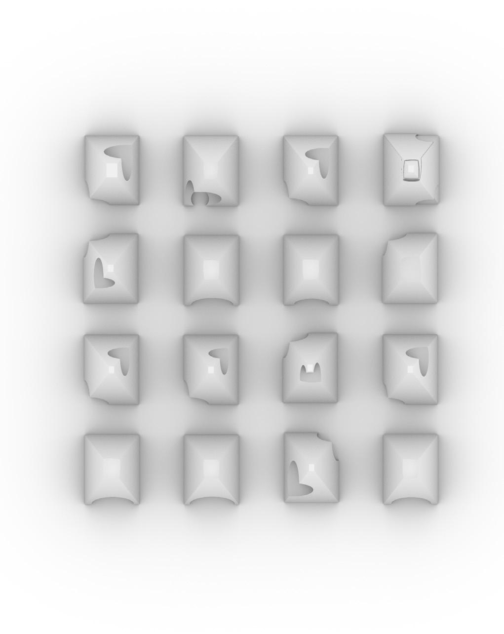
Sculpting Volumes from a Geometry

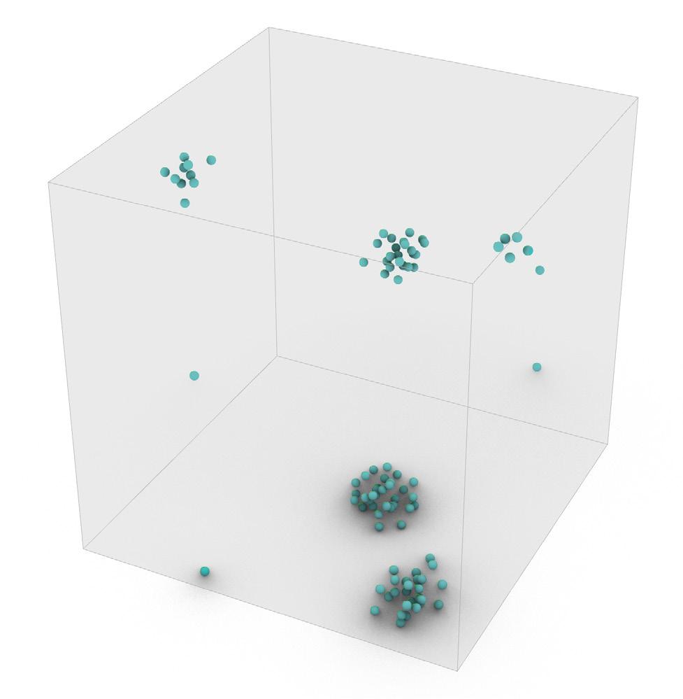
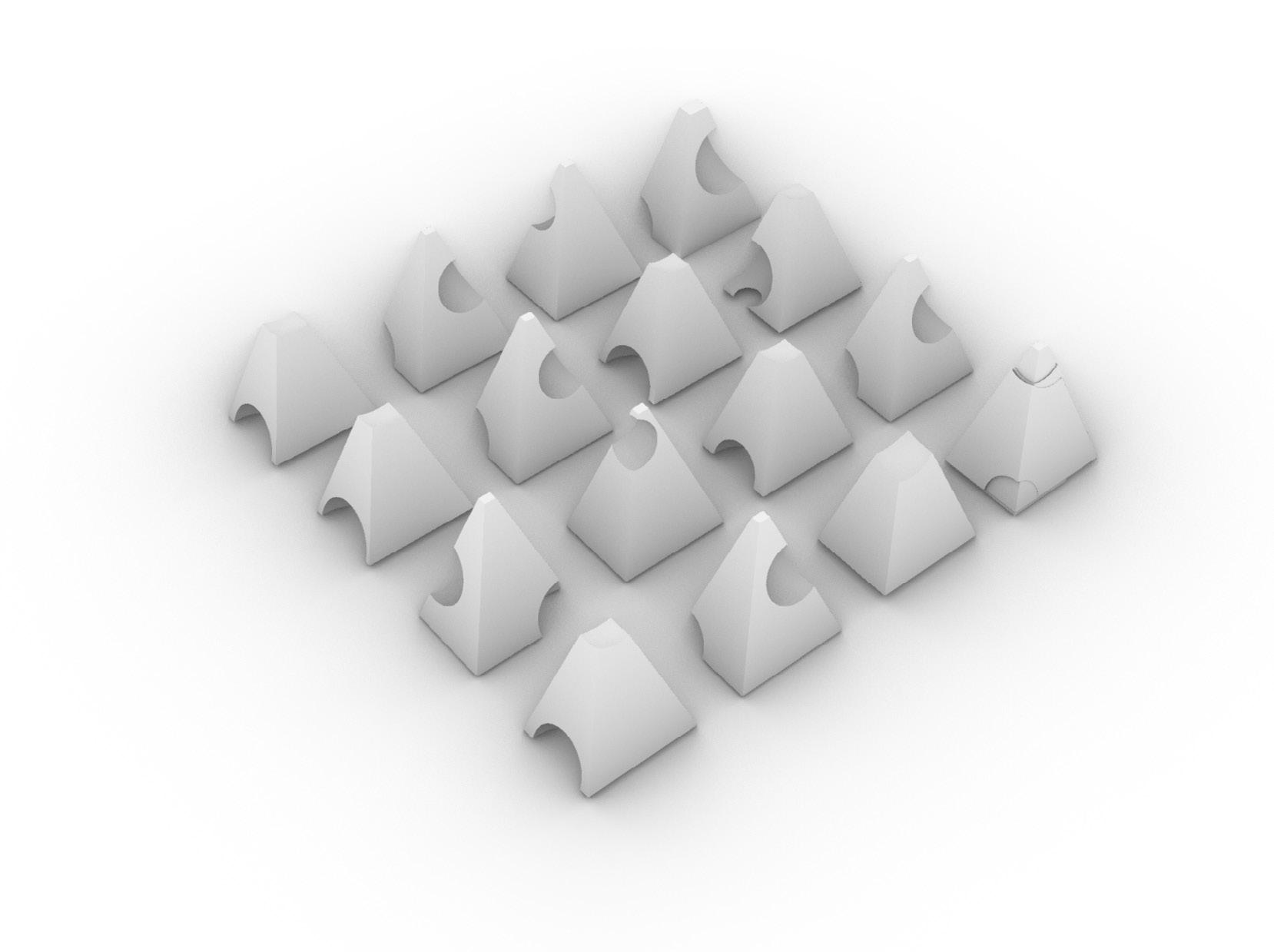
Octopus optimises the sculpted volumes based on the numbers of the factor of scaling, the seed of the populate geometry and the radius of the spheres (gene pool). It uses the number container of the minimum volume to the sculpted, maximum radius and minimum changing volume.
Populating the Geometry with Points


For creating Spheres.
Solid Difference to sculpt out the spheres from the mass.
Octopus
44 7.2 OCTOPUS - VOLUME
OPTIMISATION
45
Anahita Ghatage
F.Y. Digital Architecture , B.N.C.A | Semester 02
Tutors : Kaushik Sardesai | Vinita Wagh | Supriya Dhamale

