
Contents Chapter 1 Basic Concepts of Instrumentation 6 Chapter 2 Basic Sensors and Principles 10 Chapter 3 Amplifiers and Signal Processing 16 Chapter 4 The Origin of Biopotentials 22 Chapter 5 Biopotential Electrodes 32 Chapter 6 Biopotential Amplifiers 42 Chapter 7 Blood Pressure and Sound 56 Chapter 8 Measurement of Flow and Volume of Blood 64 Chapter 9 Measurements of the Respiratory System 72 Chapter 10 Chemical Biosensors 83 Chapter 11 Clinical Laboratory Instrumentation 84 Chapter 12 Medical Imaging Systems 86 Chapter 13 Therapeutic and Prosthetic Devices 91 Chapter 14 Electrical Safety 102 Medical Instrumentation Application and Design 4th Edition Webster Solutions Manual Full Download: http://testbanktip.com/download/medical-instrumentation-application-and-design-4th-edition-webster-solutions-manual/ Download all pages and all chapters at: TestBankTip.com
Chapter 1
Basic Concepts of Medical Instrumentation
Walter H. Olson1.1 The following table shows % reading and % full scale for each data point. There is no need to do a least squares fit.
Inspection of these data reveals that all data points are within the "funnel" (Fig. 1.4b) given by the following independent nonlinearity = ±2.4% reading or ±0.5% of full scale, whichever is greater. Signs are not important because a symmetrical result is required. Note that simple % reading = ±11.1% and simple % full scale = 2.5%.
1.2 The following table shows calculations using equation (1.8).
1.3 The simple RC high-pass filter:
The first order differential equation is:
r = 121.795 (7.701)(15.82) = 0.9997
C R + Vout+ VinI
C d x(t) – y(t) dt = y(t) R CD + 1 R y(t) = (CD) x(t) y(D) x(D) = D D + 1 RC Operational transfer function Inputs 0.50 1.50 2.00 5.00 10.00 Outputs 0.90 3.05 4.00 9.90 20.50 Ideal Output 1.00 3.00 4.00 10.00 20.00 Difference – 0.10 +0.05 0.0 – 0.10 +0.50 % Reading 11.1 1.6 % 0% – 1.0% +2.4 % = Difference/Output × 100 Full Scale – 0.5% 0.25% 0% – 0.50% + 2.5% = Difference/20 × 100 Inputs Xi 0.50 1.50 2.00 5.00 10.00 �� = 3.8 Outputs Yi 0.90 3.05 4.00 9.90 20.50 �� = 7.6 Xi – �� – 3.3 – 2.3 – 1.8 1.2 6.2 Yi – �� – 6.7 – 4.55 – 3.6 2.3 12.9 (Xi – ��)(Yi – ��) 22.11 10.465 6.48 2.76 79.98 (Xi – ��)2 10.89 5.29 3.24 1.44 38.44 (Yi – ��)2 44.89 20.7 12.96 5.29 166.41
;where 1/RC is the corner frequency in rad/s.
1.4 For sinusoidal wing motion the low-pass sinusoidal transfer function is
For 5% error the magnitude must not drop below 0.95 K or
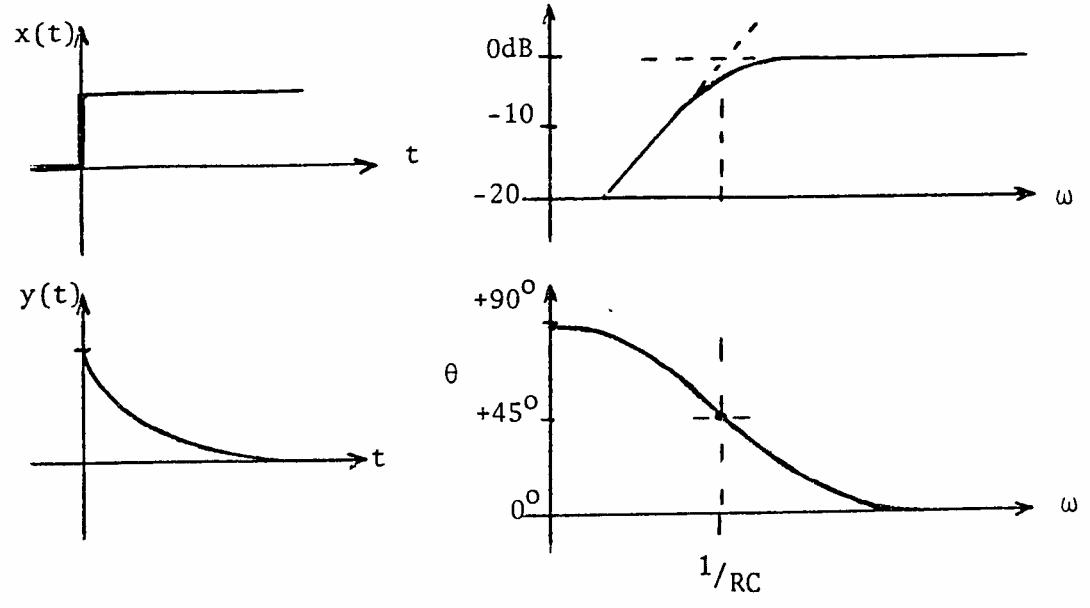
Y(j) X(j) = jRC jRC + 1 = RC (RC)2 + 1 = Arctan 1 RC
Y(j) X(j)
(j
= K
+ 1)
K j + 1 = K 2 2 + 1 =
K Solve for with = 2f = 2(100) ( 2 2 + 1) (.95 )2 = 1 = 1 – (0.95)2 (0.95)2(2100)2 1/2 = 0.52 ms Phase angle = tan–1 (–) at 50z 50 = tan–1 (–2 50 0.0005) = –9.3 at 100 Hz 100 = tan–1 (–2 100 0.0005) = –18.2
0.95
1.5 The static sensitivity will be the increase in volume of the mercury per C divided by the cross-sectional area of the thin stem
Vb = unknown volume of the bulb
cross-sectional area of the column
1.6 Find the spring scale (Fig. 1.11a) transfer function when the mass is negligible. Equation 1.24 becomes B dy(t) dt + Ks y(t) = x(t)
When M = 0. This is a first order system with
K = static sensitivity = 1 Ks
= time constant = B Ks
Thus the operational transfer function is
x(D) = 1/Ks 1 + B
D = 1 Ks + BD
and the sinusoidal transfer function becomes
1.7 a dy dt + bx + c + dy = edy dt + fx + g
(a – e)dy dt + dy = (b + f)x + (g– c)
This has the same form as equation 1.15 if g = c.
(
D + 1)y = Kx
= HgVb Ac =
C where HgVb = 1.82 10–4 cm 3 cm 3 C
Ac
Ac = π(0.1 mm)2 = π × 10–4 cm2 Thus Vb = AcK Hg = 10–4cm 2 0.2 cm/C 1.82 10–4 cm 3 cm 3C = 0.345 cm 3
K
2mm/
=
y(D)
Ks
y(j) x(j)
1 +j
Ks D
s 1 + 2B2 Ks 2 = tan–1 – B Ks
= 1/Ks
B
= 1/K
1.8 For a first order instrument
a – e d D + 1 y = b + f d x Thus = a – e d
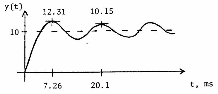
Y(j ) X(j ) = K (j + 1) K (j + 1) = K 2 2 + 1 = 0.93 K 2 2 + 1 (0.93)2 = 1 f = 1 2 = 1 2 1 – (0.93)2 (0.93)2 (.02)2 = 3.15 Hz = tan–1 (–) = –21.6 1.9 y(t) = K Ke–nt 1 – 2 sin 1 – 2 nt + where = sin–1 1 – 2 = 0.4; fn = 85 Hz tn = 3 2 – n 1 – 2 = 7.26 ms tn+1 = 7 2 – n 1 – 2 = 20.1 ms y(tn) = 10 + 10 1 – 2 e – ntn y(tn+1) = 10 + 10 1 – 2 e – ntn+1 = 12.31 = 10.15 1.10. At the maxima yn, yn+2, yn+4: sin ( ) = –1 at 3 2 , 7 2 , 11 2 and 1 – 2 ntn + = 3 2 tn = 3 2 – n 1 – 2
Chapter 2
Basic Sensors and Principles
Robert
at the minima yn+1, yn+3 …: sin ( ) = + 1 at 5 2 , 9 2 and 1 – 2 ntn+1 + = 5 2 tn+1 = 5 2 – n 1 – 2 then form the ratio yn yn+1 = K 1 – 2 e –ntn K 1 – 2 e –ntn+1 = exp –3 2 –5 2 1 – 2 = exp 1 – 2 = ln yn yn+1 = 1 – 2 Solve for
A. Peura and John G. Webster
Let the wiper fraction F = xi/xt vo/vi = Rm||FRp Rm||FRP + (1–F)RP = Rm F Rp Rm + F Rp Rm F RP Rm + F Rp + (1–F)RP = 1 1 + Rm F Rp Rm + F Rp (1–F)RP = 1 RmF + Rm + F Rp – F Rm – FFRp RmF = 1 1 + F Rp/Rm – FFRP/Rm F
2.1
2.2 The resolution of the translational potentiometer is 0.05 to 0.025 mm. The angular resolution is a function of the diameter, D, of the wiper arm and would = (translational resolution/πD) × 360. In this case the resolution is 2.87/D to 5.73/D degrees where D is in mm.

= Rp
m
=
o
i = F –1 1/F + (1–F) = F –F 1 + F – F2 =F–(F)(1 + F– F2)–1 d/dF(error) = 0 = 1–(1) (1+F–F2)–1 – (F) (–1) (1+F–F2)–2(–2F) multiply by (1+F–F2)2 0 = (1+F–F2)2 – (1+F–F2) + (F) ( – 2F) expand, ignoring terms of 2 , 3 , ... 0 = 1 + 2F – 2F2 – 1 – F + eF2 + F – 2F2 0 = –3F2 + 2F = () (F) (2–3F) F = 0, 2/3 error = 0.67 –1 1/0.67 + (1 – 0.67) = 0.67 –1 1.5 + 0.33 = 0.22 1.5 + 0.33 ≈ 0.15= 0.15 Rp/Rm
Let
/R
error
F – v
/v
= 1 1 F + Rp Rm (1–F)
A multiturn potentiometer may be used to increase the resolution of a rotational potentiometer. The increased resolution is achieved by the gearing between the shaft whose motion is measured and the potentiometer shaft.
2.3. The elastic-resistance strain gage is nonlinear for large extensions (30%), has a dead band linearity due to slackness and is subject to long-term creep. Continuity in the mercury column and between the column and electrodes may be a problem. The gage has a high temperature drift coefficient. The dynamic response and finite mechanical resistance may cause distortion. These problems may be minimized by carefully selecting the proper size gage for the extremity. The gage should be slightly extended at minimum displacement when applied to eliminate the slackness problem. Mercury continuity checks may be made using an ohmmeter. The temperature drift problems may be minimized with continual calibration or by making measurements in a controlled temperature environment.
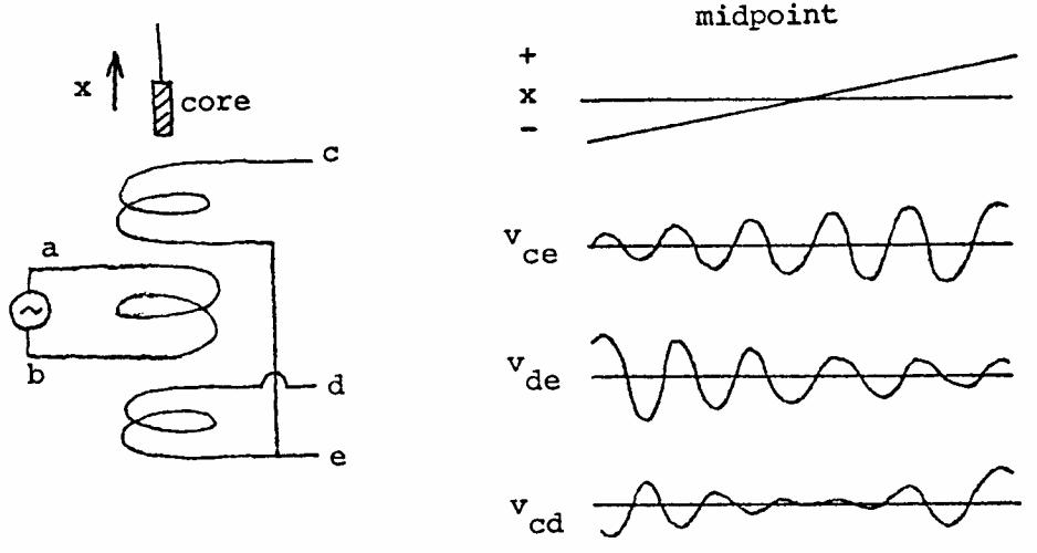
2.7 There is always a voltage induced in each secondary, because it acts as the secondary of an air-core transformer. This voltage increases when the core is inside it.
From (2.21) E = 38.7T + (0.082/2)T2 = 38.7T + 0.041T2 T C 38.7T µV 0.41T2 µV E µV 0 0 0 0 10 387 4 391 20 774 16 790 30 1161 37 1196 40 1548 66 1614 50 1935 102 2037 The second term is small. The curve is almost linear but slightly concave upward. 2.5 From (2.22) α = dE/dT = a + bt = 38.7 + 0.082T µV/˚C = 38.7 + 0.082(37) = 41.7 µV/˚C 2.6 From (2.24) = – /T2 = –4000 (300)2 = –4.4%/K
2.4
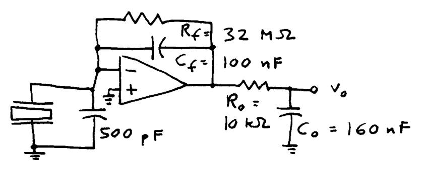
2.8 In Example 2.3 C = 500 pF for the piezoelectric transducer. The amplifier input impedance = 5 MΩ.
F = 0.05 Hz = 1 2RCequivalent
Thus Cequivalent = 0.637 × 10–6 = Cpiezoelectric + Cshunt
Cshunt = 0.636 µF = 636 nF
Q = CV, where charge Q is fixed, capacitance C increases by 636 nF/0.5 nF = 1272 times. Voltage V (sensitivity) decreases by 1/1272.
The sensitivity will be decreased by a factor of 1272 due to increase in the equivalent capacitance.
2.9 Select a feedback Cf = 100 nF (much larger than 500 pF). To achieve low corner frequency, add Rf = 1/(2πfcCf) = 1/(2π·0.05·100 nF) = 32 MΩ. To achieve high corner frequency add separate passive filter or active filter with Ro = 10 kΩ and Co = 1/(2πfcRo) = 1/(2π·100·10 kΩ) = 160 nF.
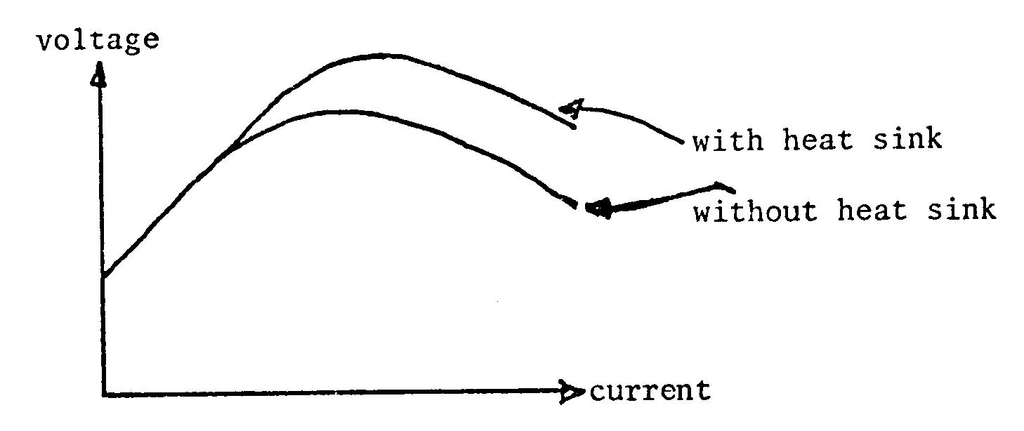
2.10 Typical thermistor V–i characteristics with and without a heat sink are shown below.
For low currents Ohm's law applies and the current is directly proportional to the applied voltage in both cases. The thermistor temperature is that of its surroundings. The system with a heat sink can reach higher current levels and still remain in a linear portion of the v–i curve since the heat sink keeps the thermistor at approximately the ambient temperature. Eventually the thermistor–heat sink combination will self heat and a negative-resistance relationship will result.
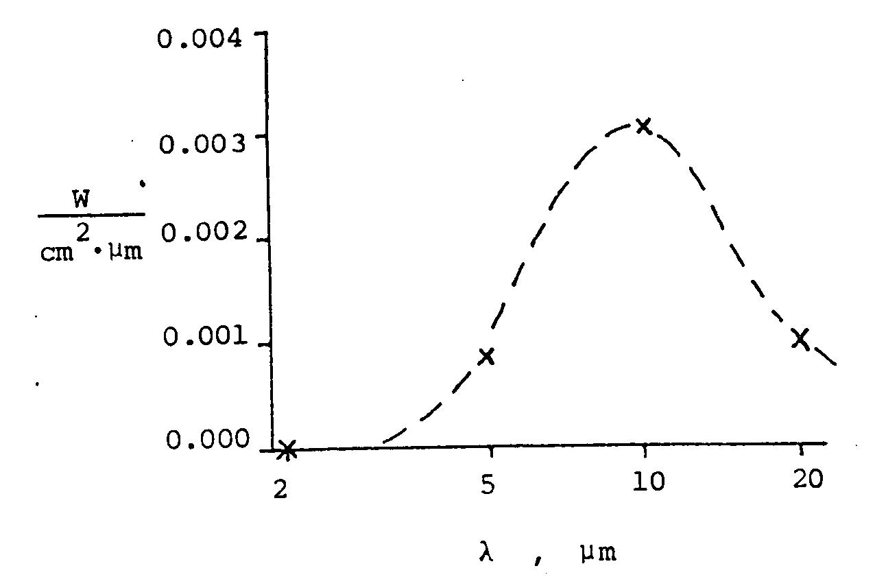
2.11 Assume = 1.0 and use (2.25).
W = 37400/[5(exp(14400/300) – 1)]
W = 37400/[5(exp(48/) – 1)]
W2 = 37400/[(32)(225 × 106)] = 0.000005
W5 = 37400/[3125)(15000] = 0.0008
W10 = 37400/[100000)(120)] = 0.003
W20 = 37400/[3.2 × 106)(11 – 1)] = 0.001
2.12
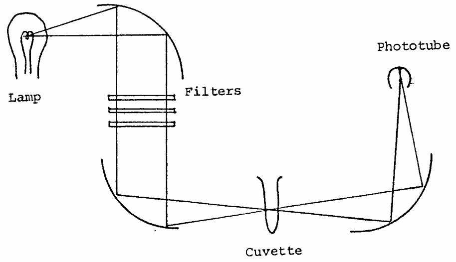
 Infrared and ultraviolet are passed better by mirrors because the absorption in the glass lenses is eliminated.
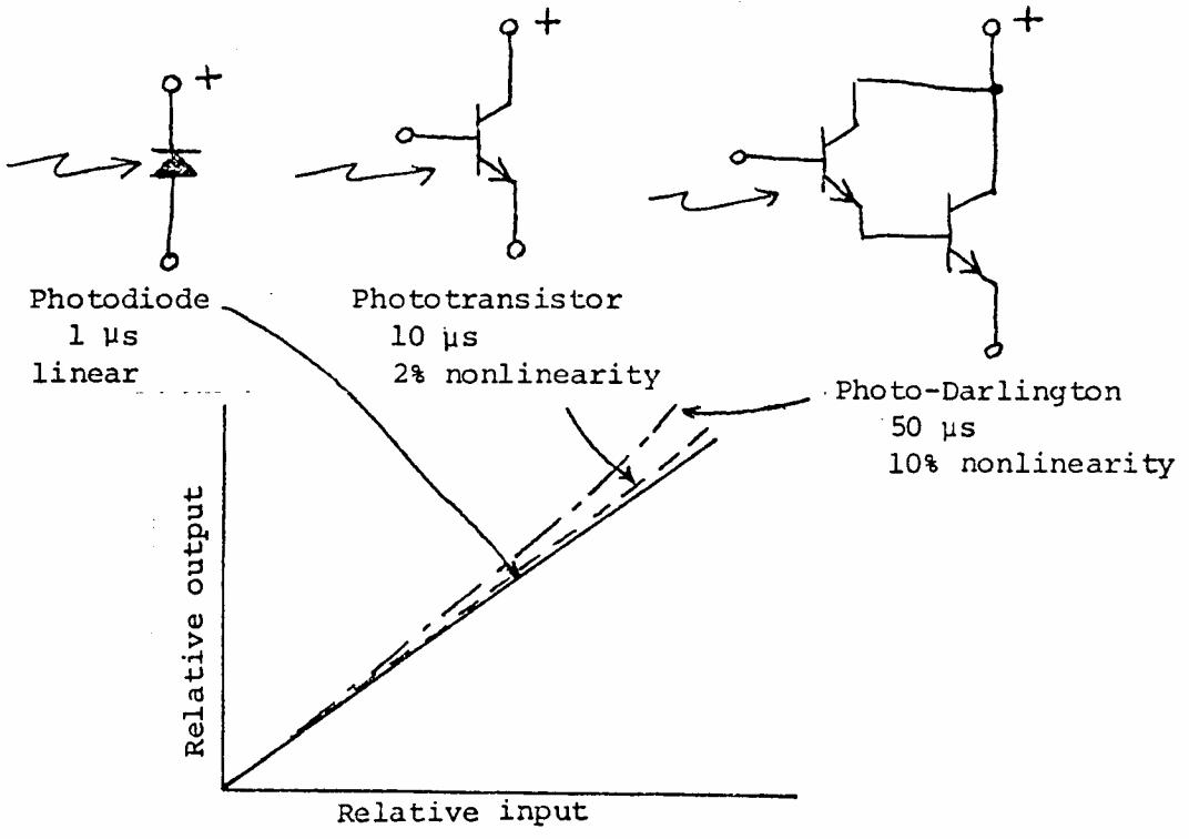
2.13 See section 2.16, photojunction devices. For small currents, beta, the current gain, increases with collector current. This produces the concave nonlinearity shown. Both nonlinearity and response time increase in the photo-Darlington because two transistors are involved.
2.14 Try several load resistors as shown by the dashed load lines following. The maximum power is 2.5 µW. The load resistor, R = V/I = (0.5 V)/(5 µA) = 100 kΩ.
2.15 (a) shows the problem the RC product is too high. (b) shows the simplest solution the transistor input resistance is much lower than R. (c) shows that an op amp provides a virtual ground that provides a low input resistance. (d) shows that if R is divided by 10, the gain may be achieved by a noninverting amplifier. Active components must have adequate speed.

Instrumentation
4th
Download: http://testbanktip.com/download/medical-instrumentation-application-and-design-4th-edition-webster-solutions-manual/ Download all pages and all chapters at: TestBankTip.com
Medical
Application and Design
Edition Webster Solutions Manual Full