Introduction to Bayesian optimization
This chapter covers
What motivates Bayesian optimization and how it works
Real-life examples of Bayesian optimization problems
A toy example of Bayesian optimization in action
You’ve made a wonderful choice reading this book, and I’m excited for your upcoming journey! On a high level, is an optimization technique that may be applied when Bayesian optimization the function (or, in general, any process that generates an output when an input is passed in) one is trying to optimize is a black box and expensive to evaluate in terms of time, money, or other resources. This setup encompasses many important tasks, including hyperparameter tuning, which we define shortly. Using Bayesian optimization can accelerate this search procedure and help us locate the optimum of the function as quickly as possible.
While Bayesian optimization has enjoyed enduring interest from the machine learning (ML) research community, it’s not as commonly used or talked about as other ML topics in practice. But why? Some might say Bayesian optimization has a steep learning curve: one needs to understand calculus, use some probability, and be an overall experienced ML researcher to use Bayesian optimization in an application. The goal of this book is to dispel the idea that Bayesian optimization is difficult to use and show that the technology is more intuitive and accessible than one would think.
Throughout this book, we encounter many illustrations, plots, and–of course–code, which aim to make the topic of discussion more straightforward and concrete. We learn how each component of Bayesian optimization works on a high level and how to implement them using state-of-the-art
libraries in Python. The accompanying code also serves to help you hit the ground running with your own projects, as the Bayesian optimization framework is very general and "plug and play." The exercises are also helpful in this regard.
Generally, I hope this book is useful for your ML needs and is an overall fun read. Before we dive into the actual content, let’s take some time to discuss the problem that Bayesian optimization sets out to solve.
1.1 Finding the optimum of an expensive black box function
As mentioned previously, hyperparameter tuning in ML is one of the most common applications of Bayesian optimization. We explore this problem, as well as a couple of others, in this section as an example of the general problem of black box optimization. This will help us understand why Bayesian optimization is needed.
1.1.1 Hyperparameter tuning as an example of an expensive black box optimization problem
Say we want to train a neural network on a large data set, but we are not sure how many layers this neural net should have. We know that the architecture of a neural net is a make-or-break factor in deep learning (DL), so we perform some initial testing and obtain the results shown in . table 1.1
Table 1.1An example of a hyperparameter tuning task m
Our task is to decide how many layers the neural network should have in the next trial in the search for the highest accuracy. It’s difficult to decide which number we should try next. The best accuracy we have found, 81%, is good, but we think we can do better with a different number of layers. Unfortunately, the boss has set a deadline to finish implementing the model. Since training a neural net on our large data set takes several days, we only have a few trials remaining before we need to decide how many layers our network should have. With that in mind, we want to know what other values we should try, so we can find the number of layers that provides the highest possible accuracy.
This task, in which we want to find the best setting (hyperparameter values) for our model to optimize some performance metric, such as predictive accuracy, is typically called in ML. In our example, the hyperparameter of our neural net is its depth hyperparameter tuning (the number of layers). If we are working with a decision tree, common hyperparameters are the maximum depth, the minimum number of points per node, and the split criterion. With a
support-vector machine, we could tune the regularization term and the kernel. Since the performance of a model very much depends on its hyperparameters, hyperparameter tuning is an important component of any ML pipeline.
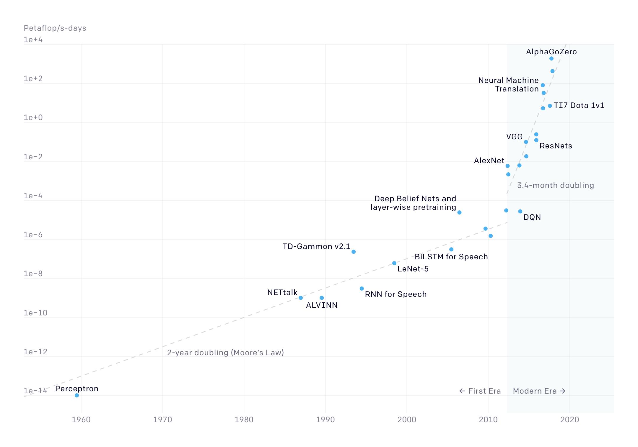
If this were a typical real-world data set, this process could take a lot of time and resources. from OpenAI () shows that as neural figure 1.1https://openai.com/blog/ai-and-compute/ networks keep getting larger and deeper, the amount of computation necessary (measured in petaflop/s-days) increases .exponentially
Figure 1.1 The compute cost of training large neural networks has been steadily growing, making hyperparameter tuning increasingly difficult.
This is to say that training a model on a large data set is quite involved and takes significant effort. Further, we want to identify the hyperparameter values that give the best accuracy, so training will have to be done many times. How should we go about choosing which values to parameterize our model, so we can zero in on the best combination as quickly as possible? That is the central question of hyperparameter tuning.
Getting back to our neural net example in , what number of layers we should try next, so table 1.1 we can find an accuracy greater than 81%? Some value between 10 layers and 20 layers is promising, since at both 10 and 20, we have more than 5 layers. But what exact value we should inspect next is still not obvious, since there may still be a lot of variability in numbers between 10 and 20. When we say , we implicitly talk about our uncertainty regarding how the variability ©Manning Publications Co. To comment go to liveBook https://livebook.manning.com/#!/book/bayesian-optimization-in-action/discussion
test accuracy of our model behaves as a function of the number of layers. Even though we know 10 layers lead to 81% and 20 layers lead to 75%, we cannot say for certain what value, say, 15 layers would yield. This is to say we need to account for our level of uncertainty when considering these values between 10 and 20.
Further, what if some number greater than 20 gives us the highest accuracy possible? This is the case for many large data sets, where a sufficient depth is necessary for a neural net to learn anything useful. Or though unlikely, what if a small number of layers (fewer than 5) is actually what we need?
How should we explore these different options in a principled way, so when our time runs out and we have to report back to our boss, we can be sufficiently confident that we have arrived at the best number of layers for our model? This question is an example of the expensive black box problem, which we discuss next.
optimization
1.1.2 The problem of expensive black box optimization
In this subsection, we formally introduce the problem of expensive black box optimization, which is what Bayesian optimization aims to solve. Understanding why this is such a difficult problem will help us understand why Bayesian optimization is preferred over simpler, more naïve approaches, such as grid search (where we divide the search space into equal segments) or random search (where we leverage randomness to guide our search).
In this problem, we have black box access to a function (some input–output mechanism), and our task is to find the input that maximizes the output of this function. The function is often called the , as optimizing it is our objective and we want to find the of the objective functionoptimum objective function—the input that yields the highest function value.
SIDEBAR Characteristics of the objective function
The term necessitates that we don’t know what the underlyingblack box formula of the objective is; all we have access to is the function output when we make an observation by computing the function value at some input. In our neural net example, we don’t know how the accuracy of our model will change if we increase the number of layers one by one (otherwise, we would just pick the best one).
The problem is expensive because in many cases, making an observation (evaluating the objective at some location) is prohibitively costly, rendering a naïve approach, such as an exhaustive search, intractable. In ML and, especially, DL, time is usually the main constraint, as we already discussed.
Hyperparameter tuning belongs to this class of expensive black box optimization problems, but it is not the only one! Any procedure in which we are trying to find some settings or parameters to
optimize a process without knowing how the different settings influence and control the result of the process qualifies as a black box optimization problem. Further, trying out a particular setting and observing its result on the target process (the objective function) is time-consuming, expensive, or costly in some other sense.
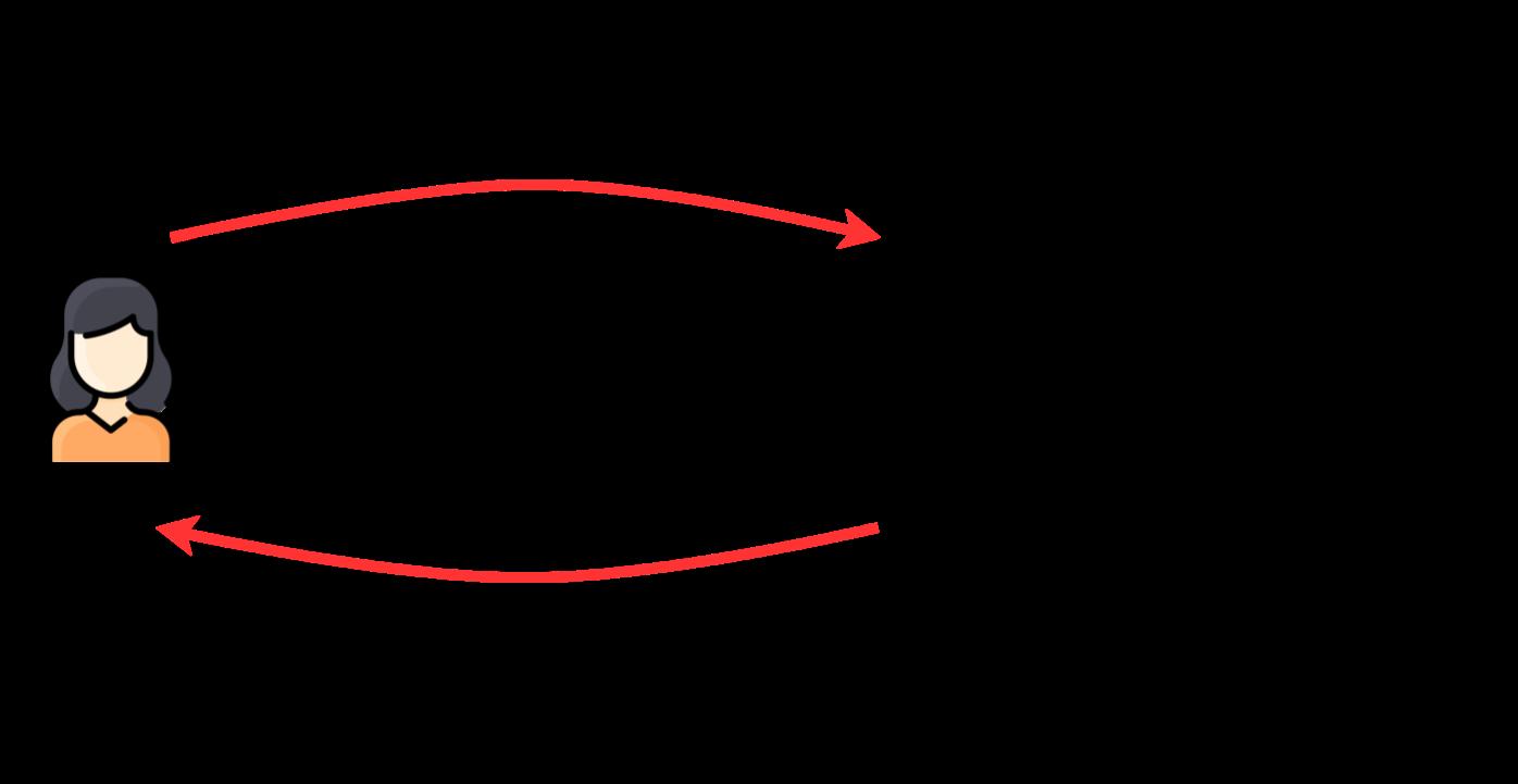
IMPORTANT The act of trying out a particular setting—that is, evaluating the value of the objective function at some input—is called or making a queryquerying the . The entire procedure is summarized in .objective function figure 1.2
Figure 1.2 The framework of a black box optimization problem. We repeatedly query the function values at various locations to find the global optimum.
1.1.3 Other real-world examples of expensive black box optimization problems
Now, let’s consider a few real-world examples that fall into the category of expensive black box optimization problems. We will see that such problems are common in the field; we often find ourselves with a function we’d like to optimize but that can only be evaluated a small number of times. In these cases, we’d like to find a way to intelligently choose where to evaluate the function.
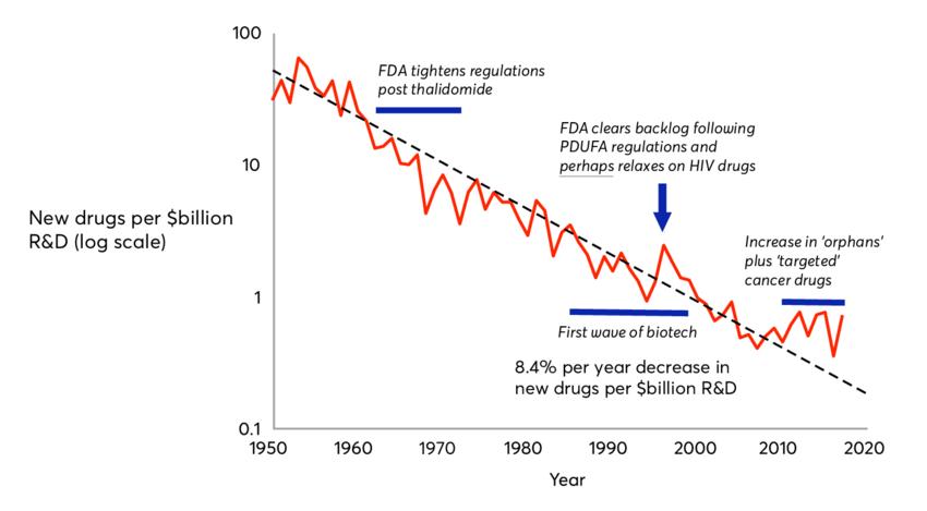
The first example is drug discovery—the process in which scientists and chemists identify compounds with desirable chemical properties that may be synthesized into drugs. As you can imagine, the experimental process is quite involved and costs a lot of money. Another factor that makes this drug discovery task daunting is the decreasing trend in the productivity of drug discovery R&D that has been robustly observed in recent years. This phenomenon is known as —a reverse of —which roughly states that the number of new drugs Eroom’s lawMoore’s law approved per billion US dollars halves over a fixed period of time. Eroom’s law is visualized in
from a paper (see "Diagnosing the Decline in Pharmaceutical R&D Efficiency" figure 1.3 Nature by Jack W. Scannell, Alex Blanckley, Helen Boldon, and Brian Warrington, ), where drug discovery throughput resulting from each https://www.nature.com/articles/nrd3681 billion-dollar investment decreases on the logarithmic scale. This scale means the decrease in throughput is exponential.
Figure 1.3 Eroom’s law dictates that it will cost increasingly more money to produce effective drugs; therefore, drug discovery is also a fundamentally hard problem.
The same problem, in fact, applies to any scientific discovery task in which scientists search for new chemicals, materials, or designs that are rare, novel, and useful, with respect to some metric, using experiments that require top-of-the-line equipment and may take days or weeks to finish. In other words, they are trying to optimize for their respective objective functions, where evaluations are extremely expensive.
As an illustration, shows a couple of data points in a real-life data set from such a task. table 1.2
The objective is to find the alloy composition (from the four parent elements) with the lowest mixing temperature, which is a black box optimization problem. Here, materials scientists worked with compositions of alloys of lead (Pb), tin (Sn), germanium (Ge), and manganese (Mn). Each given combination of percentages of these compositions corresponds to a potential alloy that could be synthesized and experimented on in a laboratory.
Table 1.2Data from a materials discovery task, extracted from the author’s research m work
% of Pb% of Sn% of Ge% of MnMixing temp. 0.500.500.000.00192.08 0.330.330.330.00258.30
As a low temperature of mixing indicates a stable, valuable structure for the alloy, the objective is to find compositions whose mixing temperatures are as low as possible. But there is one bottleneck: determining this mixing temperature for a given alloy generally takes days. The question we set out to solve algorithmically is similar: given the data set we see, what is the next composition we should experiment with (in terms of how much lead, tin, germanium, and manganese should be present) to find the minimum temperature of mixing?
Another example is in mining and oil drilling, or, more specifically, finding the region within a big area that has the highest yield of valuable minerals or oil. This involves extensive planning, investment, and labor—again an expensive undertaking. As digging operations have significant negative impacts on the environment, there are regulations in place to reduce mining activities, placing a limit on the number of that may be done in this optimization function evaluations problem.
The central question in expensive black box optimization is this: what is a good way to decide where to evaluate this objective function, so its optimum may be found at the end of the search?
As we see in a later example, simple heuristics—such as random or grid search, which are approaches implemented by popular Python packages like Scikit-learn—may lead to wasteful evaluations of the objective function and, thus, overall poor optimization performance. This is where Bayesian optimization comes into play.
1.2 Introducing Bayesian optimization
With the problem of expensive black box optimization in mind, we now introduce Bayesian optimization as a solution to this problem. This gives us a high-level idea of what Bayesian optimization is and how it leverages probabilistic ML to optimize expensive black box functions.
IMPORTANT Bayesian optimization is an ML technique that simultaneously maintains a predictive model to learn about the objective function makes decisionsand about how to acquire new data to refine our knowledge about the objective, using Bayesian probability and decision theory.
By , we mean input–output pairs, each mapping an input value to the value of the objective data
function at that input. This data is different, in the specific case of hyperparameter tuning, from the training data for the ML model we aim to tune.
In a Bayesian optimization procedure, we make decisions based on the recommendation of a Bayesian optimization algorithm. Once we have taken the Bayesian optimization-recommended action, the Bayesian optimization model is updated based on the result of that action and proceeds to recommend the next action to take. This process repeats until we are confident we have zeroed in on the optimal action.
There are two main components of this workflow:
1.
2.
An ML model that learns from the observations we make and makes predictions about the values of the objective functions on unseen data points
An optimization policy that makes decisions about where to make the next observation by evaluating the objective to locate the optimum
We introduce each of these components in the following subsection.
1.2.1 Modeling with a Gaussian process
Bayesian optimization works by first fitting a predictive ML model on the objective function we are trying to optimize—sometimes, this is called the surrogate model, as it acts as a surrogate between what we believe the function to be from our observations and the function itself. The role of this predictive model is very important, as its predictions inform the decisions made by a Bayesian optimization algorithm and, therefore, directly affect optimization performance.
In almost all cases, a Gaussian process (GP) is employed for this role of the predictive model, which we examine in this subsection. On a high level, a GP, like any other ML model, operates under the tenet that similar data points produce similar predictions. GPs might not be the most popular class of models, compared to, say, ridge regression, decision trees, support vector machines, or neural networks. However, as we see time and again throughout this book, GPs come with a unique and essential feature: they do not produce point estimate predictions like the other models mentioned; instead, their predictions are in the form of . probability distributions Predictions, in the form of probability distributions or probabilistic predictions, are key in Bayesian optimization, allowing us to quantify uncertainty in our predictions, which, in turn, improves our risk–reward tradeoff when making decisions.
Let’s first see what a GP looks like when we train it on a dataset. As an example, say we are interested in training a model to learn from the data set in , which is visualized as black table 1.3 _x_s in . figure 1.4
Table 1.3An example regression dataset corresponding to m figure 1.4
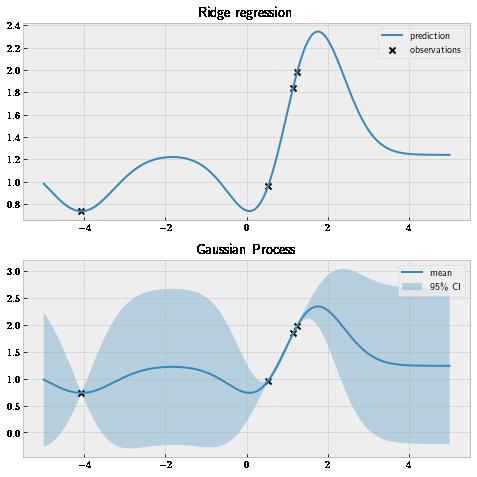
Figure 1.4 Non-Bayesian models, such as ridge regressors, make pointwise estimates, while GPs produce probability distributions as predictions. GPs, thus, offer a calibrated quantification of uncertainty, which is an important factor when making high-risk decisions.
We first fit a ridge regression model on this dataset and make predictions within a range of -5 and 5; the top panel of shows these predictions. A is a figure 1.4 ridge regression model modified version of a linear regression model, where the weights of the model are regularized so that small values are preferred to prevent overfitting. Each prediction made by this model at a given test point is a single-valued number, which does not capture our level of uncertainty about how the function we are learning from behaves. For example, given the test point at 2, this model simply predicts 2.2.
We don’t need to go into too much detail about the inner workings of this model. The point here
is that a ridge regressor produces point estimates without a measure of uncertainty, which is also the case for many ML models, such as support vector machines, decision trees, and neural networks.
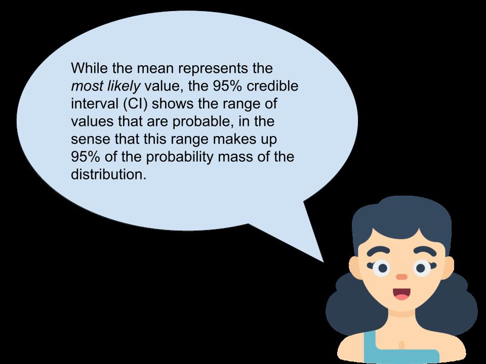
How, then, does a GP make its predictions? As shown on the bottom panel of , figure 1.4 predictions by a GP are in the form of probability distributions (specifically, normal distributions). This means at each test point, we have a mean prediction (the solid line) as well as what’s called the 95% credible interval, or CI (the shaded region).
Note that the acronym is often used to abbreviate in frequentist statistics; CIconfidence interval throughout this book, we use exclusively to denote . Many things can be said CIcredible interval about the technical differences between the two concepts, but on a high level, we can still think of this CI as a range in which it’s likely that a quantity of interest (in this case, the true value of the function we’re predicting) falls.
SIDEBAR Gaussian process versus ridge regression
Interestingly, when using the same covariance function (also known as the ), a GP and a ridge regression model produce the same predictionskernel (mean predictions for the GP), as illustrated in . We discuss figure 1.4 covariance functions in greater depth in chapter 3. This is to say that a GP receives all the benefits a ridge regression model possesses, while offering the additional CI predictions.
Effectively, this CI measures our level of uncertainty about the value at each test location. If a location has a large predictive CI (at -2 or 4 in , for example), then there is a wider figure 1.4 range of values that are probable for this value. In other words, we have higher uncertainty about this value. If a location has a narrow CI (0 or 2, in ), then we are more confident about figure 1.4 the value at this location. A nice feature of the GP is that for each point in the training data, the predictive CI is close to 0, indicating we don’t have any uncertainty about its value. This makes sense; after all, we already know what that value is from the training set.
SIDEBAR Noisy function evaluations
While not the case in , it’s possible that the labels of the data points figure 1.4 in our dataset are noisy. It’s very possible that in many situations in the real world, the process of observing data can be corrupted by noise. In these cases, we can further specify the noise level with the GP, and the CI at the observed data points will not collapse to 0 but, instead, to the specified noise level. This goes to show the flexibility modeling with GPs offers.
This ability to assign a number to our level of uncertainty, which is called uncertainty , is quite useful in any high-risk decision-making procedure, such as Bayesian quantification optimization. Imagine, again, the scenario in , where we tune the number of layers in our table 1.1 neural net, and we only have time to try out one more model. Let’s say after being trained on ©Manning Publications Co. To comment go to liveBook https://livebook.manning.com/#!/book/bayesian-optimization-in-action/discussion
those data points, a GP predicts that 25 layers will give a mean accuracy of 0.85 and the corresponding 95% CI is (0.81, 0.89). On the other hand, with 15 layers, the GP predicts our accuracy will also be 0.85 on average, but the 95% CI is (0.84, 0.86). Here, it’s quite reasonable to prefer 15 layers, even though both numbers have the same expected value. This is because we are more 15 will give us a good result. certain
To be clear, a GP does not make any decision for us, but it does offer us a means to do so with its probabilistic predictions. Decision-making is left to the second part of the Bayesian optimization framework: the policy.
1.2.2 Making decisions with a Bayesian optimization policy
In addition to a GP as a predictive model, in Bayesian optimization, we also need a decision-making procedure, which we explore in this subsection. This is the second component of Bayesian optimization, which takes in the predictions made by the GP model and reasons about how to best evaluate the objective function, so the optimum may be located efficiently.
As mentioned previously, a prediction with a (0.84, 0.86) CI is considered better than one with (0.81, 0.89), especially if we only have one more try. This is because the former is more of a sure thing, guaranteed to get us a good result. How should we make this decision in a more general case, in which the two points might have different predictive means and predictive levels of uncertainty?
This is exactly what a Bayesian optimization helps us do: quantify the usefulness of a policy point, given its predictive probability distribution. The job of a policy is to take in the GP model, which represents our belief about the objective function, and assign each data point with a score denoting how helpful that point is in helping us identify the global optimum. This score is sometimes called the . Our job is then to pick out the point that maximizes this acquisition score acquisition score and evaluate the objective function at that point.
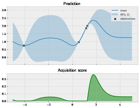
We see the same GP in that we have in , where the bottom panel shows the figure 1.5 figure 1.4 plot of how a particular Bayesian optimization policy called _Expected Improvement_ scores each point on the _x_-axis between -5 and 5 (which is our search space). We learn what this name means and how the policy scores data points in chapter 4. For now, let's just keep in mind that if a point has a large acquisition score, this point is valuable for locating the global optimum.
Figure 1.5 A Bayesian optimization policy scores each individual data point by its usefulness in locating the global optimum. The policy prefers high predictive values (where the payoff is more likely) as well as high uncertainty (where the payoff may be large).
In , the best point is around 1.8, which makes sense, as according to our GP in the top figure 1.5 panel, that’s also where we achieve the highest predictive mean. This means we will then pick this point at 1.8 to evaluate our objective, hoping to improve from the highest value we have collected.
We should note that this is not a one-time procedure but, instead, a . At each learning loop iteration of the loop, we train a GP on the data we have observed from the objective, run a Bayesian optimization policy on this GP to obtain a recommendation that will hopefully help us identify the global optimum, make an observation at the recommended location, add the new point to our training data, and repeat the entire procedure until we reach some condition for terminating. Things might be getting a bit confusing, so it is time for us to take a step back and look at the bigger picture of Bayesian optimization.
SIDEBAR Connection to design of experiments
The description of Bayesian optimization at this point might remind you of the concept of (DoE) in statistics, which sets out to solvedesign of experiments the same problem of optimizing an objective function by tweaking the controllable settings. Many connections exist between these two techniques, but Bayesian optimization can be seen as a more general approach than DoE that is powered by the ML model GP.
1.2.3 Combining the Gaussian process and the optimization policy to form the optimization loop
In this subsection, we tie in everything we have described so far and make the procedure more concrete. We see the Bayesian optimization workflow as a whole and better understand how the various components work with each other.
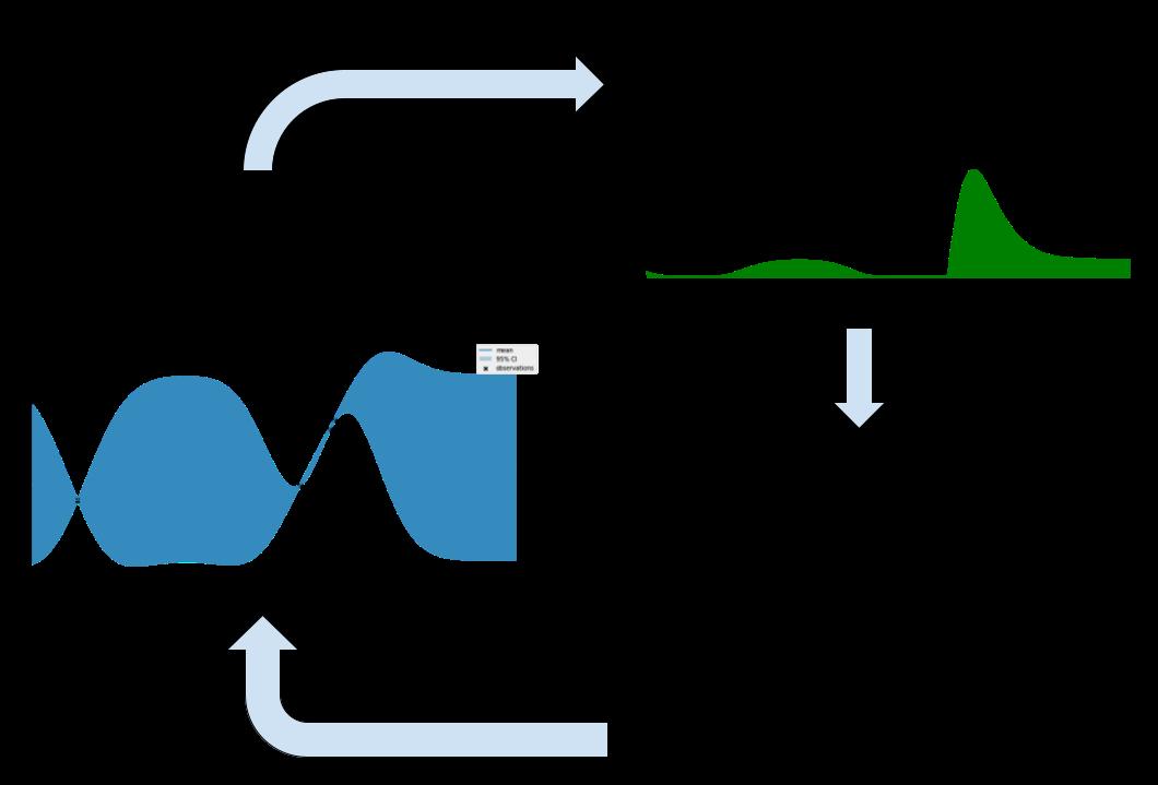
We start with an initial dataset, like those in , , and . Then, the table 1.1 table 1.2 table 1.3 Bayesian optimization workflow is visualized in , which is summarized as follows: figure 1.6
1. 2.
We train a GP model on this set, which gives us a belief about what our objective looks like everywhere, based on what we have observed from the training data. This belief is represented by the solid curve and shaded region, like those in and . figure 1.4 figure 1.5
A Bayesian optimization policy then takes in this GP and scores each point in the domain in terms of how valuable the point is in helping us locate the global optimum. This is indicated by the green curve, as in . figure 1.5
3. 4.
The point that maximizes this score is the point we will choose to evaluate the objective at next and is then added to our training data set.
The process repeats, until we cannot afford to evaluate the objective anymore.
Figure 1.6 The Bayesian optimization loop, which combines a GP for modeling and a policy for decision-making. This complete workflow may now be used to optimize black box functions.
Unlike a supervised learning task in which we just fit a predictive model on a training dataset and make predictions on a test set (which only encapsulates steps 1 and 2), a Bayesian
optimization workflow is what is typically called . a subfield in active learningActive learning ML in which we get to decide which data points our model learns from, and that decision-making process is, in turn, informed by the model itself.
As we have said, the GP and the policy are the two main components of this Bayesian optimization procedure. If the GP does not model the objective well, then we will not be able to do a good job informing the policy of the information contained in the training data. On the other hand, if the policy is not good at assigning high scores to "good" points and low scores to "bad" points (where here means helpful at locating the global optimum), then our subsequent good decisions will be misguided and will most likely achieve bad results.
In other words, without a good predictive model, such as a GP, we won’t be able to make good predictions with calibrated uncertainty. Without a policy, we can make good , but we predictions won’t make good .decisions
An example we consider multiple times throughout this book is weather forecasting. Imagine a scenario in which you are trying to decide whether to bring an umbrella with you before leaving the house to go to work, and you then look at the weather forecasting app on your phone.
Needless to say, the predictions made by the app need to be accurate and reliable, so you can confidently base your decisions on them. An app that always predicts sunny weather just won’t do. Further, you need a sensible way to make decisions from these predictions. Never bringing an umbrella, regardless of how likely rainy weather is, is a bad decision-making policy and will get you in trouble when it does rain. On the other hand, always bringing an umbrella, even with 100% sunny weather, is also not a smart decision. You want to decide to bring your adaptively umbrella, based on the weather forecast.
Adaptively making decisions is what Bayesian optimization is all about, and to do it effectively, we need both a good predictive model and a good decision-making policy. Care needs to go into both components of the framework; this is why the two main parts of the book, following this chapter, cover modeling with GPs and decision-making with Bayesian optimization policies, respectively.
1.2.4 Bayesian optimization in action
At this point, you might be wondering if all of this heavy machinery really works—or works better than some simple strategy like random sampling. To find out, let’s take a look at a "demo" of Bayesian optimization on a simple function. This will also be a good way for us to move away from the abstract to the concrete and tease out what we are able to do in future chapters.
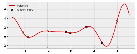
Let’s say the black box objective function we are trying to optimize (specifically, in this case, maximize) is the one-dimensional function in , defined from -5 to 5. Again, this picture figure 1.7 is only for our reference; in black box optimization, we, in fact, do not know the shape of the
objective. We see the objective has a couple of local maxima around -5—roughly, -2.4 and 1.5—but the global maximum is on the right at approximately 4.3. Let’s also assume we are allowed to evaluate the objective function a maximum of 10 times.
Figure 1.7 The objective function that is to be maximized, where random search wastes resources on unpromising regions.
Before we see how Bayesian optimization solves this optimization problem, let’s look at two baseline strategies. The first is a random search, where we uniformly sample between -5 and 5; whatever points we end up with are the locations we will evaluate the objective at. is figure 1.7 the result of one such scheme. The point with the highest value found here is at roughly = 4, x having the value of () = 3.38. fx
SIDEBAR How random search works
Random search involves choosing points uniformly at random within the domain of our objective function. That is, the probability we end up at a point within the domain is equal to the probability we end up at any other point. Instead of uniform sampling, we can draw these random samples from a non-uniform distribution if we believe there are important regions in the search space we should give more focus to. However, this non-uniform strategy requires knowing which regions are important, before starting the search.
Something you might find unsatisfactory about these randomly sampled points is that many of them happen to fall into the region around 0. Of course, it’s only by chance that many random samples cluster around 0, and in another instance of the search, we might find many samples in another area. However, the possibility remains that we could waste valuable resources inspecting a small region of the function with many evaluations. Intuitively, it is more beneficial to spread out our evaluations, so we learn more about the objective function.
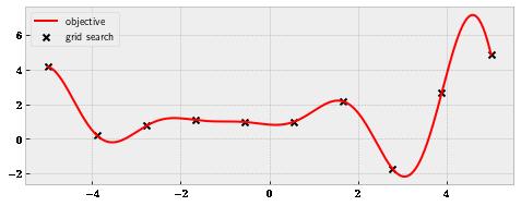
This idea of evaluations leads us to the second baseline: grid search. Here, we spreading out divide our search space into evenly spaced segments and evaluate at the endpoints of those segments, as in . figure 1.8
Figure 1.8 Grid search is still inefficient at narrowing down a good region.
The best point from this search is the very last point on the right at 5, evaluating at roughly 4.86. This is better than random search but is still missing the actual global optimum.
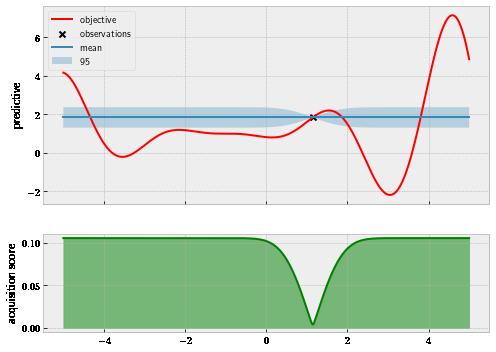
Now, we are ready to look at Bayesian optimization in action! Bayesian optimization starts off with a randomly sampled point, just like random search, shown in . figure 1.9
Figure 1.9 The start of Bayesian optimization is similar to random search.
The top panel represents the GP trained on the evaluated point, while the bottom panel shows the score computed by the Expected Improvement policy. Remember this score tells us how much we should value each location in our search space, and we should pick the one that gives the highest score to evaluate next. Interestingly enough, our policy at this point tells us that almost the entire range between -5 and 5 we’re searching within is promising (except for the region around 1, where we have made a query). This should make intuitive sense, as we have only seen one data point and we don’t yet know how the rest of the objective function looks in other areas. ©Manning Publications Co. To comment go to liveBook https://livebook.manning.com/#!/book/bayesian-optimization-in-action/discussion
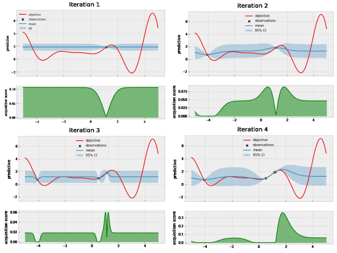
Our policy tells us we should explore more! Let’s now look at the state of our model from this first query to the fourth query in . figure 1.10
Figure 1.10 After four queries, we have identified the second-best optimum.
Three out of four queries are concentrating around the point 1, where there is a local optimum, and we also see that our policy is suggesting to query yet another point in this area next. At this point, you might be worried we will get stuck in this locally optimal area and fail to break out to find the true optimum, but we will see this is not the case. Let’s fast-forward to the next two iterations in . figure 1.11
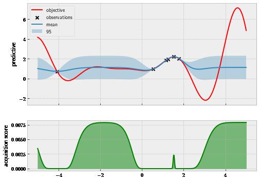
Figure 1.11 After exploring a local optimum sufficiently, we are encouraged to look at other areas.
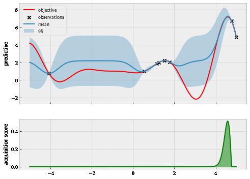
After having five queries to scope out this locally optimal region, our policy decides there are other, more promising regions to explore—namely, the one to the left around -2 and the one to the right around 4. This is very reassuring, as it shows that once we have explored a region enough, Bayesian optimization does not get stuck in that region. Let’s now see what happens after eight queries in . figure 1.12
Figure 1.12 Bayesian optimization successfully ignores the large region on the left.
©Manning Publications Co. To comment go to liveBook https://livebook.manning.com/#!/book/bayesian-optimization-in-action/discussion
Here, we have observed two more points on the right, which update both our GP model and our policy. Looking at the mean function (the solid line, representing the most likely prediction), we see that it almost matches with the true objective function from 4 to 5. Further, our policy (the green curve) is now pointing very close to the global optimum and basically no other area. This is interesting because we have not thoroughly inspected the area on the left (we only have one observation to the left of 0), but our model believes that regardless of how the function looks like in that area, it is not worth investigating compared to the current region. This is, in fact, true in our case here.
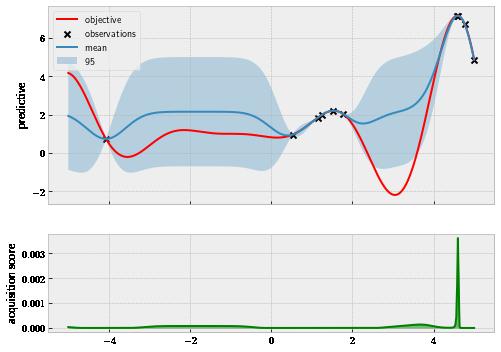
Finally, at the end of the search with 10 queries, our workflow is now visualized in . figure 1.13 There is now little doubt that we have identified the global optimum around 4.3.
Figure 1.13 Bayesian optimization has found the global optimum at the end of the search.
This example has clearly shown us that Bayesian optimization can work a lot better than random search and grid search. This should be a very encouraging sign for us, considering that the latter two strategies are what many ML practitioners use when faced with a hyperparameter tuning problem.
For example, Scikit-learn is one of the most popular ML libraries in Python, and it offers the module for various model selection tasks, including hyperparameter tuning. model_selection However, random search and grid search are the only hyperparameter tuning methods implemented in the module. In other words, if we are indeed tuning our hyperparameters with random or grid search, there is a lot of headroom to do better.
Overall, employing Bayesian optimization may result in a drastic improvement in optimization ©Manning Publications Co. To comment go to liveBook https://livebook.manning.com/#!/book/bayesian-optimization-in-action/discussion
performance. We can take a quick look at a couple of real-world examples:
A research paper entitled "Bayesian Optimization is Superior to Random Search for Machine Learning Hyperparameter Tuning" (2020, https://arxiv.org/pdf/2104.10201.pdf), which was the result of a joint study by Facebook, Twitter, Intel, and others, found that Bayesian optimization was extremely successful across many hyperparameter tuning tasks.
Frances Arnold, Nobel Prize winner in 2018 and professor at Caltech, uses Bayesian optimization in her research to guide the search for enzymes efficient at catalyzing desirable chemical reactions.
A study entitled "Design of Efficient Molecular Organic Light-Emitting Diodes by a High-Throughput Virtual Screening and Experimental Approach" ( ) published in applied Bayesian https://www.nature.com/articles/nmat4717 Nature optimization to the problem of screening for molecular organic light-emitting diodes (an important type of molecules) and observed a large improvement in efficiency.
And there are many more of these examples out there.
SIDEBAR
When not to use Bayesian optimization
It’s also important to know when the problem setting isn’t appropriate and when to use Bayesian optimization. As we have said, Bayesiannot optimization is useful when our limited resources prevent us from evaluating the objective function many times. If this is not the case, and evaluating the objective is cheap, we have no reason to be frugal with how we observe the objective function.
Here, if we can inspect the objective thoroughly across a dense grid, that will ensure the global optimum is located. Otherwise, other strategies, such as the DIRECT algorithm or evolutionary algorithms, which are algorithms that often excel at optimization when evaluations are cheap, may be used. Further, if information about the gradient of the objective is available, gradient-based algorithms will be better suited.
I hope this chapter was able to whet your appetite and get you excited for what’s to come. In the next section, we summarize the key skills you will be learning throughout the book.
1.3 What will you learn in this book?
This book provides a deep understanding of the Gaussian process model and the Bayesian optimization task. You will learn how to implement a Bayesian optimization pipeline in Python using state-of-the-art tools and libraries. You will also be exposed to a wide range of modeling and optimization strategies when approaching a Bayesian optimization task. By the end of the book, you will be able to do the following:
Implement high-performance Gaussian process models using GPyTorch, the premiere GP modeling tool in Python; visualize and evaluate their predictions; choose appropriate
©Manning Publications Co. To comment go to liveBook https://livebook.manning.com/#!/book/bayesian-optimization-in-action/discussion
parameters for these models; and implement extensions, such as variational Gaussian processes and Bayesian neural networks, to scale to big data
Implement a wide range of Bayesian optimization policies using the state-of-the-art Bayesian optimization library BoTorch, which integrates nicely with GPyTorch, and inspect as well as understand their decision-making strategies
Approach different specialized settings, such as batch, constrained, and multiobjective optimization, using the Bayesian optimization framework
Apply Bayesian optimization to a real-life task, such as tuning the hyperparameters of an ML model
Further, we use real-world examples and data in the exercises to consolidate what we learn in each chapter. Throughout the book, we run our algorithms on the same data set in many different settings, so we can compare and analyze the different approaches taken.
1.4 Summary
Many problems in the real world may be cast as expensive black box optimization problems. In these problems, we only observe the function values, without any additional information. Further, observing one function value is expensive, rendering many cost-blind optimization algorithms unusable.
Bayesian optimization is an ML technique that solves this black box optimization problem by designing intelligent evaluations of the objective function, so the optimum may be found as quickly as possible.
In Bayesian optimization, a Gaussian process acts as a predictive model, predicting what the value of the objective function is at a given location. A Gaussian process produces not only a mean prediction but also a 95% credible interval, representing uncertainty via normal distributions.
To optimize a black box function, a Bayesian optimization policy iteratively makes decisions about where to evaluate the objective function. The policy does this by quantifying how helpful each data point is in terms of optimization.
A Gaussian process and a policy go hand in hand in Bayesian optimization. The former is needed to make good predictions, and the latter is needed to make good decisions. By making decisions in an adaptive manner, Bayesian optimization is better at optimization than random search or grid search, which are often used as the default strategies in black box optimization problems.
Bayesian optimization has seen significant success in hyperparameter tuning in ML and other scientific applications, such as drug discovery.