Solutions Manual for Viscous Fluid Flow 4th Edition White by areLeaders

Solutions Manual for Viscous Fluid Flow 4th Edition White Solutions Manual for Viscous Fluid Flow 4th Edition White

SOLUTIONS for Viscous Fluid Flow 4th Edition by White

CHAPTER 1. PRELIMINARY CONCEPTS

1-1 A 1.4-cm diameter sphere placed in a freestream at 18 m/s at 20°C and 1 atm. Compute the diameter Reynolds number for 3 cases:

(a) Air: Table A-2 - at 20°C, 3 1.205kg/m, 1.81== E-5 Pa-s. Then

(b) Water: Table A-1 - at 20°C, 3 998kg/m, 1.002mPa-s:==

== 251,000

kg/m. === From Table 1-2 for hydrogen,

1-2 At what wind velocity will an 8-mm-diameter wire “sing” at middle C (256 Hz)?

For air at 20°C, assume 2 v1.5E-5 m/s.  From Fig. 1-8 guess a vortex-shedding Strouhal number of 0.2 [check the Reynolds number afterward]. Then ( )( )/U fD/U0.22560.008,orU10.24m/s. = At this speed the Reynolds number is ( )( ) D ReUD/v10.240.0081.5E / -55400.=== This is nicely in the range where fD/U0.2. = Perhaps we could iterate just a little more closely to obtain fD/U0.205, ReUD/v5300, orU/== 10.0ms (Ans.)

1-3 If U12 m/s = in Prob. 1-2 above, what is the wire drag in N/m?

For air assume 32 and 1.205kg/mv1.5E-5m/s.== The Reynolds number is ( )( ) ( ) D ReUD/v120.008/l.5E-56400 ===

PROBLEM SOLUTIONS

( )( )(

ReVD/

===

(Ans.)

)

1.205180.014

1.81E-5

16,800

( )( )( ) ( ) D Re998180.014/0.001002

(Ans.)

( ) ( )( )

== Then ( )( )( ) ( ) D Re0.0838180.0148.83E/ 6 == 2,400 (Ans.)

p/RT101350/41242930.0838

n068

T/T8.411E-6293/2738.83E-6Pa-s

Solutions Manual for Viscous Fluid Flow 4th Edition White Solutions Manual for Viscous Fluid Flow 4th Edition White

From Fig. 1-9 at this Reynolds number, estimate a drag coefficient of 1.1. Then

1-4 Given, without proof, the Poiseuille-paraboloid laminar-pipe-flow formula from Chap. 3, 22 C/( u()Rr), =−  find the wall shear stress if max u30m/s, D1== cm, and 0.3kg/(m-s).

[The exact analysis will be given in Sect. 3-3.1.]

Examining the formula, we see that the maximum velocity occurs on the centerline:

With C thus known for this data, we may evaluate wall shear stress by differentiation:

We should check the Reynolds number DRe but we don’t know the density. But “oil” is usually in the range 3 900kg/m.

Then

well within the laminar-flow range.

1-5 Glycerin at 20C is confined between two large parallel plates. One plate is fixed and the other moves parallel at 17 mm/s. The distance between the plates is 3 mm. Assuming no-slip, estimate the shear stress in the glycerin, in Pa

Solution: Glycerin at 20Cis confined between two large parallel plates. One plate is fixed and the other moves parallel at 17 mm/s V = The distance h between the plates is 3 mm.

For glycerin at 20C, the viscosity 1.5kg/ms  =

distribution without the prior consent of McGraw Hill LLC. -2-

( ) ( )( )( ) ( )( ) 2 2 dragD 1 FCVDL1.10.51.205120.0081.0/ 2  ===   0.76Nm (Ans.)

=

( ) ( ) ( ) ( ) 2 222 mx uur0 CR/30m/sC0.005/0.3,or:C3.6E5N/m-s======

( )( ) wall r0 u2RC 2RC20.0053.6E5 r =   =====   3600Pa (Ans.)

( )( )( ) ( ) Dmax ReuD/900300.0103 / . == 900,  which



Moving plate Fixed plate h Glycerin u = V u =0 Solutions Manual for Viscous Fluid Flow 4th Edition White Solutions Manual for Viscous Fluid Flow 4th Edition White

Assuming no-slip, the shear stress

1-6 Given a plane unsteady viscous flow in polar coordinates:

Compute the vorticity and sketch some profiles of vorticity and velocity.

From Appendix B, the vorticity is

The instantaneous velocity and vorticity profiles are plotted at top. Att0, = the flow is a “line” vortex, irrotational everywhere except at the origin ( ).

1-7 Given the two-dimensional unsteady flow ( ) ( ) ux/1+t,vy/1+2t, == find the equation for the streamlines which pass through the point 00 (x,y) at time ( ) t0. = From the geometric requirement for two-dimensional streamlines at any instant,

McGraw Hill LLC.

or distribution without the prior

-3-

No reproduction

consent

( )( ) ( ) 3 3 1.5kg/ms1710 m/s 8.5Pa 310 m/s V h    ===  . (Ans.)

2 r Cr v0;v1expr4vt    ==−−     

( ) 2 z 1Cr rvexp rr2vt4vt    ==−   

=

Solutions Manual for Viscous Fluid Flow 4th Edition White Solutions Manual for Viscous Fluid Flow 4th Edition White

Holding time t constant, we may separate the variables and integrate to obtain n

n1t/12t. =++ To satisfy the initial condition, we must have

= where (

Cy/x. = The final result for the (unsteady) streamlines is

1-8 For the inviscid streamline approaching the forward stagnation point of the cylinder in Fig. 1-5, evaluate the strain rates and the time to go from (

Then, from Appendix B, evaluate the normal and shear-strain rates along the line :=

The particle moving toward the stagnation point gets shorter in the “r” direction and fatter by the same amount in the “  ” direction, thus maintaining constant volume for this incompressible flow. The shear strain rate is zero because we are on a line of symmetry.

For part (b), by definition, the radial velocity along the stagnation line ( )= is

We may separate the variables and integrate to find the time of travel between ( )2R and ( ) R:

McGraw Hill LLC.

or distribution without the prior

-4( ) ( ) streamline y1t dyv dxux12t + == +

consent

yCx,

)n 00

n 00 yx1t ,n yx12t  + ==  +  (Ans.)

) ( )

(

) ( ) 2R, toR,  From Eqs. (1-2), ( ) ( ) 2222 r vU1R/rcosθ,vU1R/rsinθ =−=−+

22 r rr 33 22 r 33 v2URcos2UR | rrr vv2URcos2UR 1 | rrrr  =   =  ===−    =+=−=+  2 r r 3 vv 1v4URsin|0 rrr r   =   =+−==  (Ans. a)

( )22 r dr vU1R/r dt  ==−−

R R 2 22 2R 2R UtrlnrdrRrR 2rR rR  −  −==+=−   + −   (Ans. b) Solutions Manual for Viscous Fluid Flow 4th Edition White Solutions Manual for Viscous Fluid Flow 4th Edition White

It takes infinite time to actually reach the stagnation point, where V0 =

1-9 Use the approximate equation of state for water,

with

compute the following quantities for water,

(a) the pressure required to double the density of water:

(b) the bulk modulus K of water at 1 atm. By definition,

These are accurate estimates of the measured compressibility and sound speed of water. 1-10 As shown, a plate slides down an incline on a film of oil of viscosity

(a) Estimate the terminal sliding velocity V*: Acceleration is zero, so

( )( )n oo p/pA1/A +−

A3000,n7 = to

3 oop1atm,

== :

998kg/m

( )( )7 o p/p300012.03000381128,or:p =+−== 381,000atm (Ans. a)

( ) ( ) n1 Tooo n o dpn K|pA1npA121007p at 1 datm.  ==+=+=   Thus the bulk modulus is K21,007atm 2.13E9Pa (Ans. b)

( ) 1/2 1/2 1oatm3 2.13 E9Pa aK// 998 kg/m  ===    1460ms (Ans. c)

5E-4 = slug/ft-s

WV sinθAA y  ==  Solutions Manual for Viscous Fluid Flow 4th Edition White Solutions Manual for Viscous Fluid Flow 4th Edition White

where A is the plate area touching the oil film.

Assuming a linear velocity profile, * VV= and y = the film thickness, hence

in English units Hence solve for ( ) * Vterminal/ = 1.85fts (Ans a

(b) Estimate the time for the plate to accelerate from rest to 99% terminal velocity: If x is down the incline, then a dynamic force balance gives

The solution to this first-order linear ordinary differential equation is

For our data, then, the time to reach 99% of terminal velocity is

1-11 Estimate the viscosity of nitrogen at 86 MPa and 49°C. From Appendix A-3, for 2 N, read cc T226R126K, p33.5 atm, === c 18.0 E-6 Pa-s. = At this high pressure, we cannot use “low density” formulas but rather must use Fig. 1-17. Compute ratios:

ccc T49273p86E62.55;25.3;Read 2.50.1 T126p33.5101350

Then our estimate is ( ) c 2.52.518.0-=== 45±2 μPas (Ans.)

The agreement with the measured value (also 45 Pa-s ) is excellent.

1-12 Estimate the thermal conductivity of helium at 420°C and 1 atm. This is truly “lowdensity”, since ccpp and TT. A power-law estimate would be based on 0°C:

( ) ( ) ( ) * WVV sinθ40sin30A0.00059 y0.005/12   ===    

)

x FWVWdV sinθA, ygdt dVgA or:Vg sinθ dtWy =−=    +=    

VV*1expt0.99V* if t* WygA     =−−==   

gA4.605Wy

( )( ) ( )( )( ) t* 32.20.0 4.6054 0059.0 00.005/12 == 0.53sec (Ans. b)

( )

+ ==== 

( ) ( ) 072 n oo 420273 kkT/T0.142W/m-K/273 +     0.278WmK Solutions Manual for Viscous Fluid Flow 4th Edition White Solutions Manual for Viscous Fluid Flow 4th Edition White

Alternately, we could use the kinetic theory formula, Eq. (1-41). From Appendix A-5 for helium, 2.551Å, T10.22K, and M4.003.

use Eq. (1-34) to compute

Our estimate from (1-41) then is

The agreement with the experimental value of 0.28 W/m-K is good for both estimates.

1-13 According to Table C-5 and Fig. 1-15, at what pressure is the viscosity of CO2 equal to approximately 5 3010 Pas when the temperature is 800°R ?

Thus, 25 rp = (from Fig. 1-15). Then,

1-14 Fit the given viscosity-vs-temperature data for ammonia gas to power-law and Sutherlandlaw formulas.

(a) The power-law is an excellent fit to this data. Taking o T300K, = we obtain, by least-squares to a ( ) ( ) log vs.logT plot, 

All rights

or distribution

the

of McGraw

-7-

reserved.

reproduction

without

prior consent

Hill LLC.

 ===

0.145.20 v 420273420273 1.1470.50.6226 10.2210.22 ++  ++=   [check with

1-1]

First

Table

( ) ( ) ( ) 22 v 0.0833T0.0833693 k/M2.5510.62264.003 ===  0.27 WmK

Solution: 800°R444.4444 K T = = , 548°R304.4444 K c T = = , 444.4444K 1.46 304.4444K r c T T T == = 5 30 Pas 10  =  , 5 3.43 Pas 10 c =  , 5 6 3010 Pas 8.75 34.310 Pas r c    ==  = 

pressure ( ) 72.9atm251822.5atm crppp=== . (Ans.)

o oo T 0.3%forT300K T   =    1.051 (Ans. a) Solutions Manual for Viscous Fluid Flow 4th Edition White Solutions Manual for Viscous Fluid Flow 4th Edition White

(b) The Sutherland-law is not an especially good fit to the data, which has  rising with T at an increasing rate. It may be fit to least squares by minimizing the functional

for the given six data points. The minimum is found by differentiating the functional with respect to * S,v with the result * S1.91, = or:

fit S  573°K (Ans. b)

The error is 2.4%, or eight rimes more than the power-law fit.

1-15 Experimental data for the viscosity of helium at low pressure are as follows:

Fit these values to a suitable formula.

Solution: Experimental data for the viscosity of helium in Kelvin scale at low pressure are as follows:

the

-8-

distribution without

prior consent of McGraw Hill LLC.

( ) ( ) 2 3/2 ** 6 i **** i ** ooo i1 i T1STS where,T,S TSTT =  +   −===   +   

best

T, °C 0 100 200 300 400 500 µ, Pa·s 1.87 × 10–5 2.32 × 10–5 2.73 × 10–5 3.12 × 10–5 3.48 × 10–5 3.48 × 10–5

T, K 273 373 473 573 673 773 µ, Pa·s 1.87 × 10–5 2.32 × 10–5 2.73 × 10–5 3.12 × 10–5 3.48 × 10–5 3.48 × 10–5 Using power law curve, 00 n T T   =    For 5 0 1.87 Pas 10  =  and 0 273 K T = T 373 K 473 K 573 K 673 K 773 K n 0.691 0.688 0.69 0.688 0.597 Therefore, the mean value 5 1 0.671 5 i i n n = ==  ( 4 %  accuracy for 250 K1000 K T  ). (Ans.) Solutions Manual for Viscous Fluid Flow 4th Edition White Solutions Manual for Viscous Fluid Flow 4th Edition White

1-16 Analyze newtonian flow between parallel plates (Fig. 1-15) with a finite slip velocity ( )udu/dy= l at both walls.

The velocity profile is still linear, but with slip at both walls the slope is less, as shown in the sketch:

( )du/dyVu / 2 h =−

Introducing u from the slip relation, we obtain

1-17 Derive Eq. (1-106) from a balance of forces on the differential surface-area alement shown in the problem.

Since the sliver of area is negligibly thin, it has no weight. The pressures act on a projected surface area xy dSdS. The surface tension forces are slanted slightly upward, at angles xy (d/2)and() d/2, respectively. The force balance is

For differentially small angles, ( ) sindd. = Clean up this equation and rearrange:

since, by definition, d/dS1/R, = where R is the radius of curvature.

1-18 Two bubbles of radii 12Rand R coalesce isothermally into a single bubble 3 R. Find the radius of the new (single) bubble.

Because of surface tension, the pressure inside a bubble (which has two surfaces) is higher than ambient, o pp4/R. =+ T Assuming that no interior-bubble air mass escapes during the coalescence, 123 mmm, += or, for an ideal isothermal gas of temperature T,

w duVV or: dyh2h2  == ++ll at

(Ans.)

both walls

( ) ( ) ( ) yxxyaxy 2dSsind/22dSsind/2ppdSdS0 ++−=TT

y x a x a yxy d pp d 11 p dSdSRR    +=−+    =−  TT (Ans.)

Solutions Manual for Viscous Fluid Flow 4th Edition White Solutions Manual for Viscous Fluid Flow 4th Edition White

where  is the gas constant. Canceling common terms and cleaning up, we have

This must be solved numerically or algebraically for the new radius 3R

1-19 In Prob. 1-1, if the temperature, sphere size, and velocity remain the same for air flow, at what air pressure will the Reynolds number DRe be equal to 10,000?

Solution: From Prob. 11, 293K,0.014m, 18m/s, TDV === and 1.81E-5Pa-s.=  Use the specified Reynolds number to compute the required air density:

1-20 A solid cylinder of mass m, radius R, and length L falls concentrically through a vertical tube of radius , + RR where . RR The tube is filled with gas of viscosity  and mean free path . Neglect fluid forces on the front and back faces of the cylinder and consider only shear stress in the annular region, assuming a linear velocity profile. Find an analytic expression for the terminal velocity of fall, V, of the cylinder (a) for no-slip; (b) with slip, Eq. (1-91).

Solution: (a) For no-slip, the shear stress in the thin annular region between cylinders is

(b) For slip, modify the shear stress (see Prob. 1.16 for another example):

-10-

123 4/4/4/444 333 ooo pRpRpRRRR TTT +++ +=  III

Hill LLC.

123333

( ) ( ) 323322 331212 44 +=+++ IIoo pRRpRRRR (Ans.)

( )( ) 18/0.014 Re10,000 1.81-5 /=== D msm VD Ekgms    Solve 3 0.718 / kgm  = Ideal gas: ( )( ) 0.718, 287293 === pp RT  Solve for 60400 pPakPa = 60 (Ans.)

, ==  uV yR    then ( ) 2 shearwall V WmgFARL R   ====    Solve for - 2 noslip mgR V RL  = Ans. (a)

Solutions Manual for Viscous Fluid Flow 4th Edition White Solutions Manual for Viscous Fluid Flow 4th Edition White

1-21 Solve P1-20 for the terminal fall velocity for no-slip if the cylinder is aluminum, with diameter 4 cm and length 10 cm. The tube has a diameter of 4.02 cm and is filled with argon gas at 20C.

Solution: For no-slip, the shear stress �� in the thin annular region is

1-22 In Fig. Pl-22 a disk rotates steadily inside a disk-shaped container filled with oil of viscosity .

Assume linear velocity profiles with no-slip and neglect stress on the outer edges of the disk. Find a formula for the torque M required to drive the disk.

Solution: The disk tangential velocity varies with radius, ,Vr = hence the local shear stress is / rh

on the top and bottom of the disk. The torque on a circular strip dr wide is

-11-2 , or:, 22 duVuduVV u dyRdyRR  ==== ++ As above in part (a), = wmgA  , ( ) 2 2 slip mgR V RL + = Ans. (b)

Hill LLC.

uV yR   =  =  . Then, ( ) 2 shearwallWmgFA V RL R   ====     3 2710 kg/m Al = , 0.02 m R = , 0.1m L = , 2 9.81 m/s g = ; then, 2 3.3408 N Al mgRL  == ( ) 0.0201m0.02m0.0001m RRRR =+−=−= 5 2.24 Pas 10 Ar =  Therefore, ( )( ) ( )( ) 25 1187.4431 m/s 3.3408N0.0001m 2 0.01256m2.2410 Pas noslip Ar mgR V RL   ===  (Ans.)



Fig. Pl-22

=

Solutions Manual for Viscous Fluid Flow 4th Edition White Solutions Manual for Viscous Fluid Flow 4th Edition White

1-23 Show, from Eq. (1-86), that the coefficient of thermal expansion of a perfect gas is given by 1/. = T  Use this approximation to estimate  of ammonia gas ( )3NH at 20°C and 1 atm and compare with the accepted value from a data reference.

Solution: Introduce the ideal-gas law into the definition of :

It doesn’t matter what gas we are considering, ammonia or carbon dioxide or whatever, the ideal gas approximation predicts 1/1/293K. T === -1 0.00341K Ans

This estimate is very close to estimates for ammonia in the literature, e g., White (1988).

1-24 The rotating-cylinder viscometer in Fig. P1-24 shears the fluid in a narrow clearance ,r as shown. Assuming a linear velocity distribution in the gaps, if the driving torque M is measured, find an expression for μ by (a) neglecting, and (b) including the bottom friction.

Solution: (a) Analyze the annular region only. The shear stress equals ( ) ( ) du/dy/. RR

The shear force on the cylinder side is normal to the radius, and the driving moment must be

-12( ) ( ) 2 22 r dMdArsidesrrdr h    ==   or: 4 3 0 4 R R Mrdr hh    ==  Ans.

McGraw Hill LLC.

 2 1111 −  =−=−=−==    1 T pp pp TTRTT RT    Ans.

Fig. Pl-24

Solutions Manual for Viscous Fluid Flow 4th Edition White Solutions Manual for Viscous Fluid Flow 4th Edition White

(b) On the bottom, the shear stress varies linearly

1-25 Consider 3 1 m of a fluid at 20°C and 1 atm. For an isothermal process, calculate the final density and the energy, in joules, required to compress the fluid until the pressure is 10 atm, for (a) air; and (b) water. Discuss the difference in results.

Solution: (a) The work done is ,  pd where  is the volume. From the ideal-gas law, . = pmRT  Thus

(b) For water, we could use the compressed-liquid tables, but we can estimate the (very small) result from the bulk modulus ( ) /2.23E9Pa T Kdpd == for water, Eq. (1-84). The change in volume of the water is very small when the change in pressure is only 9 atm:

A slightly more accurate estimate from Prob. 1-9, or from the compressed-liquid tables, gives 3 0.00042 m.

Then the work required to compress water from 1 atm to 10 atm is

This is 1000 times less than Ans.(a) for air above, since water is nearly incompressible.

Copyright 2022 © McGraw Hill LLC. All rights reserved. No reproduction or distribution without the prior consent of McGraw Hill LLC. -13( ) 2 3 0 2 w RRL MRdFRdARRLd RR    ====   Solve for 3 2 MR RL    =  Ans. (a)

radius: 4 3 bottom 00 2 2 2 4 RR w rR MrdArrdrrdr RRR    ====   Thus ( ) 34 total 3 2 2 , Solve 4 2 /4 RLRMR M RR RLR     =+=  + Ans. (b)

with

( )( )3 1013501ln10 1 Pam  ==   233,000J Ans (a)

( ) ( )( ) 3 3 19101350 0.0041 2.239 mPa p m KEPa      −=−−

− 

( )( ) ( )3 12 5.51013500.00042 avg WpdpPam  =−−=−−    230J Ans. (b)

2 22 1211 11 1 lnln p mRT WpddmRTp p     =−=−=−=   Solutions Manual for Viscous Fluid Flow 4th Edition White Solutions Manual for Viscous Fluid Flow 4th Edition White

1-26 Equal layers of two immiscible fluids are being sheared between a moving and a fixed plate, as in Fig. P1-26. Assuming linear velocity profiles, find an expression for the interface velocity U as a function of 12,, and. V

Solution: The shear stress is the same in each layer:

1-27 Utilize the inviscid-flow solution of flow past a cylinder, Eqs. (1-3), to (a) find the location and value of the maximum fluid acceleration max along a the cylinder surface. Is your result valid for gases and liquids? (b) Apply your formula for maxa to air flow at 10 m/s past a cylinder of diameter 1 cm and express your result as a ratio compared to the acceleration of gravity. Discuss what your result implies about the ability of fluids to withstand acceleration.

Solution: Along the cylinder surface, , = rR and Eqs. (1-3) reduce to 0 = rv and 2sin.  =− vU 

Thus, along the surface, the absolute velocity is ( ) V2sin/, UsR  = where s is the arc length along the surface, measured from the front stagnation point. There is a convective acceleration given by

(a) The acceleration is a maximum at 135, or //4.==

This result is valid for all fluids, gases or liquids, in the inviscid approximation.

(b) For the given data, 0.005 m,10 m/s,  ==RU compute, independent of fluid properties,

All

reserved. No reproduction or distribution without the prior consent of McGraw

-14-

rights

Hill LLC.



Fig. P1-26

1122 ,/2/2 === VUU hh solve for 1 12 = + UV   Ans.

2 2sincos    ==   U dVss aVU dsRRR



sR 

/.  = 2 max 2 aUR Ans. (a)

Thus

( ) ( ) 22 max 210m/s/0.005m40,000m/s a == 4080 g’s Ans. (b) Solutions Manual for Viscous Fluid Flow 4th Edition White Solutions Manual for Viscous Fluid Flow 4th Edition White

The lesson is that fluids have no fear of huge accelerations that would defeat a human being.

1-28 The coefficient of thermal expansion is defined as

Determine  for an ideal gas with pRT  = . Show your work in detail. Solution: Given, the coefficient for thermal expansion is

for ideal gas,

1-29 Starting with Maxwell’s low-density approximation of the viscosity, namely,

and Newton’s expression of the wall shear stress as a function of the velocity gradient,

, express Maxwell’s slip velocity,

(a) as a function of the shear stress, density, and speed of sound a ;

(b) as a function of the Mach number, the mean-flow velocity U , and the skin friction coefficient,

Solution: Given, Maxwell’s low-density approximation of viscosity is 2 3 a

= density, = mean free path, and a = speed of sound.

Newton’s wall shear stress �� as a function of velocity gradient is w

, where

1 p T    =−  

pRT  =

22 1111 p ppRT TRTRTRTT    =−=−−   −=−=    (Ans.)

Using

3 a   ,

w w u y    =   

w u u y   =    ,

2 2 w f C U   =

 



y    =    . Solutions Manual for Viscous Fluid Flow 4th Edition White Solutions Manual for Viscous Fluid Flow 4th Edition White

Slip velocity �� is ww u  = , and constant 

= .

Dividing by mean-flow velocity U and arranging gives

number is U Ma a = , and skin friction coefficient is

1-30 Consider a hydraulic lift with a 50 cm diameter shaft sliding inside a housing with an inside diameter of 50.02 cm. If the shaft travels at 0.25 m/s, calculate the shaft resistance to motion per unit length. You may use water as the working fluid.

1-31 Consider a thin air gap of 1mm that is formed between two parallel surfaces that are maintained at 20C and 40C, respectively. In the case of a quiescent medium (say still air), calculate the heat transfer rate across the gap per unit area.

or distribution without the prior

-16-

consent

McGraw Hill LLC.



Therefore, 3 22 3 www w w u u ya a        ===       . (Ans.)

2 32 4 ww u U UaU   =

2 2 w f C U   = Therefore, 3 4 wf uMaUC = (Ans.)

Mach

Solution

( ) 2 wallA V FRL R   ==     . 0.25 m R = , 1m L = , 0.25 m/s V = ( ) 0.251m0.25m0.001m RRRR =+−=−= 5 1.02 Pas 10 water =  (at 20C and 1atm) ( )( ) ( )( ) ( ) 5 31.0210Pas0.25 m/s20.25 m1m 4.005510N 0.001m unitlengthF  =  = (Ans.)

: Shaft resistance F to motion is

Solutions Manual for Viscous Fluid Flow 4th Edition White Solutions Manual for Viscous Fluid Flow 4th Edition White

Solution: The rate of heat transfer per unit area (in one-dimensional space) is

The parallel plates are at 20C and 40C. Then, k needs to be determined for 30C

1-32 In the presence of viscosity, the pressure drop associated with a fully developed laminar motion in a horizontal tube of length L and diameter D may be evaluated

flow rate. Show that the corresponding head loss may be written as

What value of lamf do you obtain?

Solution: Consider fully developed flow and apply steady-flow energy equation between section 1 and section 2.

Use 12zz = (horizontal), 12VV = (constant cross-section), 12  = (same velocity profile), 0 Sh = (no pump); to simplify as 12 L pp p h

reproduction or distribution

the

-17-

without

prior consent

McGraw Hill LLC.

( ) ( )TxxTx qk x +− −  .

Using power law curve, ( ) 0.81 0 0 303 K 273 K 0.0241W/mK0.0262W/mK n air T T kk   ===     . Therefore, ( ) 2 313K293K 0.0262W/mK524W/m 0.001m q  −=   . (Ans.)

One finds: 12 4 128 LQ ppp D   =−= where 

2 1 4 QDV  = denotes the volumetric

2 12 lam 2 L pp LV hfgDg  ==

analytically.

stands for the dynamic viscosity and

22 21 22 SLpVpVzzhh gggg    ++=+++− 

gg  == … (1) Q L D 1 2 Solutions Manual for Viscous Fluid Flow 4th Edition White Solutions Manual for Viscous Fluid Flow 4th Edition White

Empirical data on viscous losses in straight sections of pipe are correlated by the dimensionless

In the presence of viscosity, the pressure drop associated with a fully developed laminar motion in a horizontal tube of length L and diameter

For fully developed laminar flow, using equations (4) and (5) in equation (2) gives

1-33 A time-dependent, two-dimensional motion has three velocity components that are given by

where a and b are pure constants. The objective of this problem is to compare and contrast the streamlines in this flow with the pathlines of the fluid particles.

(a) Find the equations governing the streamline that passes through the point ( )1,1 at time t .

or distribution

the

without

prior consent of McGraw Hill LLC. -18-

Darcy friction factor 2 1 2 pD f L V  = … (2) From equation (2), 2 1 2 L pfV D  = … (3)

and

2 lam 2 L LV hf Dg = (where lamff = , for laminar flow). (Ans.)

Combining equations (1)

(3) gives

D is 12 4 128 LQ ppp D   =−= … (4) Dynamic viscosity is , and volumetric

is 2 1 4 QDV  = … (5)

flow rate

2 lam 42 1 128 26464 4 ReD LDV D f DVLVD      == (Ans.)

1 x u at = + 1 y v bt = + 0 w =

Solutions Manual for Viscous Fluid Flow 4th Edition White Solutions Manual for Viscous Fluid Flow 4th Edition White

(b) Calculate the path of a particle that starts at ( ) ( ) 000,1,1rxy== at 0 t = . Determine the location of a particle at 1 t = , denoted as 1r .

Solution: The geometric requirement for two-dimensional streamlines is as follows:

By separating the variables, 1

Solving this gives

The condition of the streamline passing through the point ( )1,1 at time t is 1 C = must be satisfied.

Therefore, the governing equation is

The rate of change of x component of particle velocity with respect to time is

By separating the variables and integrating, (

constant).

The rate of change of y component of particle velocity with respect to time is

By separating the variables and integrating, ( )

C is the integration constant).

At 0 t = , 01 1 xxC === and 02 1 yyC === .

Therefore, the path of the particle is (

( ) ( ) 1 1 yat vdy udxxbt + == +

ybtx

 =  + 

1 dyatdx

) 1 lnlnln 1 at

bt +  =+  + 

integrating, ( ) ( ) (

yxC

1 1 at bt yCx +   +  =

(where C is the integration constant).

1 1 at bt yx +   +  = … (1) (Ans.)

dxx dtat

= +

1 1 1 a xCat =+ (where 1

)

C is the integration

1 dyy dtbt

= + .

1 2 1 b

(where

yCbt =+

1 1 1 1 b a bt yx at +

+ … (2) (Ans.) Solutions Manual for Viscous Fluid Flow 4th Edition White Solutions Manual for Viscous Fluid Flow 4th Edition White

) ( )

Therefore, at 1 t = , (

Then, (

Comparing equations (1) and (2), we can say that the condition under which the streamlines coincide with pathlines is 0 ab== .

1-34 A tornado may be simulated as a two-part circulating flow in cylindrical coordinates, with 0

(a) Calculate the divergence of the velocity. Is the flow compressible or incompressible?

(b) Determine the vorticity. Is the flow rotational or irrotational?

-20-

Hill LLC.

1 1 1 a xxa ==+

( ) 1 1 1 b yyb ==+

)

and

)

) 11

abrxyab ==++ 

(Ans.)

(

111 , 1,1

(Ans.)

rz vv==

( ) ( ) 2 rrR v R rR r      =    

Solution

Divergence of velocity is ( ) ( ) ( ) 11 0 rz vrvvv rrrz    =++=  (incompressible). (Ans.) Vorticity is ( ) 111 zrzr rz rv v vvvv veee rzzrrrr          ==−+−+−      Only nonzero component of vorticity is ( ) 1 z rv rr   =  . (Ans.) For segment (1), 2 z  = (nonzero; thus rotational). (Ans.) R r vϴ (1) (2) Solutions Manual for Viscous Fluid Flow 4th Edition White Solutions Manual for Viscous Fluid Flow 4th Edition White

For

Only nonzero component of tangential strain rate is

For segment (1), 0

The sum of normal strain rate components is

1-35 In modeling the motion of an 8-meter diameter tornado rotating at an angular speed of  at the point of maximum swirl, it is possible to use the Maicke

Majdalani profile (Maicke and Majdalani 2009) as a piecewise approximation for which 0 rz vv== and the tangential velocity is given by

(a) State whether the flow is 1D, 2D, or 3D; steady or unsteady; and specify ( )vr  as r →

(b) Calculate the divergence of the velocity. Is the flow compressible or incompressible?

(d) Determine the strain rates and the shear stresses in the inner and outer flow segments.

(e) What is the limit of ( )vr  as 0 r → ? Hint: In taking the limit, it is helpful to remember that

= and that, in the inner segment, the tangential velocity can be rewritten as

the prior

distribution without

consent of McGraw Hill LLC. -21-

segment (2), 0 z = (irrotational). (Ans.)

1 2 r vv rr      =−   (Ans.)

r 

(Ans.)

2 2 r R r    =− . (Ans.)

For segment (2),

1 0 rrz rrzz v vvv rrrz        ++=+++=    (Ans.)

( ) ( ) 2

rrr vr r r     −   =    

–

161ln 01 (inner,forcedvortexsegment)

1 (outer,freevortexsegment)

( )

( ) 2 1 1ln 16 r v r     = Solution: (2) 1 r vϴ (1) 0 Solutions Manual for Viscous Fluid Flow 4th Edition White Solutions Manual for Viscous Fluid Flow 4th Edition White

' ' ln u u

The velocity varies with respect to the radial distance r from the centerline and is independent of the axial distance z or of the angular position . This represents a typical onedimensional flow. (Ans.)

distribution without the prior consent of McGraw Hill LLC. -22-

rz v vv ttt    === 

(steady). (Ans.)

r → , ( ) 0 vr  → . (Ans.) Divergence of velocity is ( ) ( ) ( ) 11 0 rz vrvvv rrrz    =++=  (incompressible). (Ans.) Vorticity is ( ) 111 zrzr rz rv v vvvv veee rzzrrrr          ==−+−+−      . Only nonzero component of vorticity is ( ) 1 z rv rr   =  For segment (1), 2 1 32ln z r   =   (rotational). (Ans.) For segment (2), 0 z = (irrotational). (Ans.) Only nonzero component of tangential strain rate is 1 2 r vv rr      =−   . For segment (1), 16 r  =− . (Ans.) For segment (2), 2 16 r r    =− . (Ans.) Then, shear stress for segment (1) is 32 r  =− and segment (2) is 2 32 r r    =− (Ans.) As 0 r → , ( ) 0 vr  → . (Ans.) Solutions Manual for Viscous Fluid Flow 4th Edition White Solutions Manual for Viscous Fluid Flow 4th Edition White

Since 0

, the flow is time invariant

1-36 The Taylor profile, which has been used to describe the bulk gaseous motion in planar, slab rocket chambers (Maicke and Majdalani 2008), corresponds to a self-similar profile in porous channels that bears symmetry with respect to the chamber’s midsection plane. Using normalized Cartesian coordinates, the streamfunction may be written as

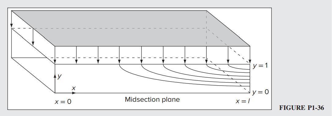
, and 0 xl

, where l represents the aspect ratio of the chamber (i.e., the length of the porous surface normalized by the chamber half height). In this problem, the velocity vector, normalized by the wall injection speed, may be expressed as V(,)ij xyuv =+ .

(a) Determine the axial and normal velocity profiles using and dd

(b) Evaluate the velocity divergence and determine whether the motion is compressible or incompressible.

Solution: The axial and normal velocity profiles of the stream function are given as follows:

1 sin 2 xy  =   ;



01 y



uv dydx  ==−

1 cos 22 dx uy dy    ==   , and 1 sin 2 d vy dx    =−=−   (Ans.) Divergence of velocity is ( ) ( ) ( ) 2 1 ,sin 42 x Vxyuvy yx     =+=−    (compressible) (Ans.) Only nonzero vorticity component is ( ) 2 1 ,sin 42 zz vux Vxyy xy      ==−=      (rotational) (Ans.) Solutions Manual for Viscous Fluid Flow 4th Edition White Solutions Manual for Viscous Fluid Flow 4th Edition White

1-37 In the Taylor flow problem described above, determine the following:

(a) The strain rates.

(

b) The Lagrangian time-dependent coordinates ( ) j xt and ( ) j yt for a particle j that enters the porous chamber at the sidewall where 1 jy = and jjxX = at 0 t = . Recall that and

(

c) The pathlines of a particle j entering the chamber at 1, 2, 3, 4, 5 j X = . Display your results in the ( ) , xy plane.

Solution: Only nonzero components of strain rate are as follows:

By separating variables and integrating,

integration constant).

Given, at 0 t = , ( ) ( ),,1 jjj xyX = .

Then, 1 j CX = , and 2 1 C = .

Therefore, the time-dependent coordinates for the particle are

jj dxdy uv dtdt ==

1 cos 22 xx u y x     ==   , 1 cos 22 yy y    =−  , and 2 1 sin 82 xy x y    =−   (Ans.) The rate of change of ( ) j xt is 11 cos 22 j jj dx uxy dt   ==   .

11 cos 22 1 j ty j xCe     = , ( 1 1 ln C    is the integration constant). The

1 sin 2 j j dy vy dt   ==−   .

rate of change of ( ) j yt is

1 2 2 4 tan t j yCe    =   , ( 2 1 ln C    is the

11 cos 22 j ty jj xXe     = and 1 2 4 tan t j ye    =   . (Ans.) Solutions Manual for Viscous Fluid Flow 4th Edition White Solutions Manual for Viscous Fluid Flow 4th Edition White

The equation of the pathline is

Pathlines of the particle j entering the chamber at 1, 2, 3, 4, 5 j X = are plotted on the ( ) , xy plane as follows:

1-38 The Taylor–Culick profile, which describes the bulk gaseous motion in solid rocket motors (Culick 1966), corresponds to an axisymmetric, self-similar profile in porous tubes. Using normalized cylindrical coordinates, the streamfunction may be written as

, where l represents the aspect ratio of the motor (i.e., the length of the porous surface normalized by the chamber radius). In this problem, the velocity vector, normalized by the wall injection speed, may be expressed as V(,) rzrz rzveve =+ .

(a) Determine the axial and radial velocity profiles using Stokes’ definition:

1 cos 2 1 tan 4 1 y j j jj y xX           =   (Ans.)

(Ans.)

2 1 sin 2 zr   =   ; 01 r  ,

0 zl

and

11 and zr vv rrrz   ==−  x y Xj =1 Xj =2 Xj =3 Xj =4 Xj =5 Solutions Manual for Viscous Fluid Flow 4th Edition White Solutions Manual for Viscous Fluid Flow 4th Edition White

(b) Evaluate the velocity divergence and determine whether the motion is compressible or incompressible.

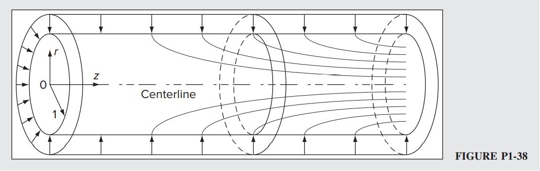
Solution: The axial and normal velocity profiles of the stream function are given as follows:

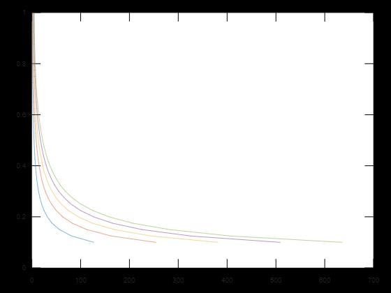
1-39 In the Taylor–Culick flow problem described above, determine the following:

(a) The strain rates.

(b) The Lagrangian time-dependent coordinates ( ) j rt and ( ) j zt for a particle j that enters the cylindrical rocket chamber at the sidewall where 1 jr = and jjzZ = at 0 t = . Recall that

Z = . Display your results in the ( ) , rz plane.

2 11 cos 2 z vzr rr     ==    and 2 111 sin 2 r vr rzr     =−=−    (Ans.) Divergence of velocity is ( ) ( ) ( ) ( ) 11 ,0 rz Vrzrvvv rrrz    =++=  (incompressible). (Ans.) Vorticity is given by ( ) ( ) 111 , zrzr rz rv v vvvv Vrzeee rzzrrrr          ==−+−+−      . Only nonzero vorticity component is 22 1 sin 2 rz vv zrr zr     =−=    (rotational) (Ans.)

and jj rz drdz vv dtdt ==

3, 4,

Solutions Manual for Viscous Fluid Flow 4th Edition White Solutions Manual for Viscous Fluid Flow 4th Edition White

By separating variables and integrating,

Given, at 0 t = , ( ) ( ) ,1, jjj rzZ = . Then,

Therefore, the time-dependent coordinates for the particle are

The equation of the pathline is

Pathlines of the particle j entering the chamber at 1, 2, 3, 4, 5 j Z = are plotted on the ( ) , rz plane as follows:

Copyright 2022 © McGraw Hill LLC. All rights reserved. No reproduction or distribution without the prior consent of McGraw Hill LLC. -27Solution: Only nonzero components of strain rate are as follows: 22 2 111 cossin 22 r rr v rr rr    ==−+   , 2 2 111 sin 2 r v v r rrr       =+=−    , 2 1 cos 2 z zz v r z    ==    , and 22111 sin 222 rz zr vv zrr zr     =+=−      (Ans.) The rate of change of ( ) j rt is 2 11 sin 2 j rj j dr vr dtr   ==−   .

separating variables and integrating, ( ) 1 1 4 tan t j rCe   = , ( 1 1 ln C    is integration constant). The rate of change of ( ) j zt is 2 1 cos 2 j zj dz vzr dt   ==   .

2 1 cos 2 2 tr j zCe     = , ( 2 1 ln C    is integration constant).

1 1 C = , and 2 j CZ = .

( ) 1 4 tan t j re   = and 2 1 cos 2 tr jj zZe     = (Ans.)

1 2 cos 2 2 1 tan 4 1 rj j jj r zZ           =   . (Ans.)

Solutions Manual for Viscous Fluid Flow 4th Edition White Solutions Manual for Viscous Fluid Flow 4th Edition White

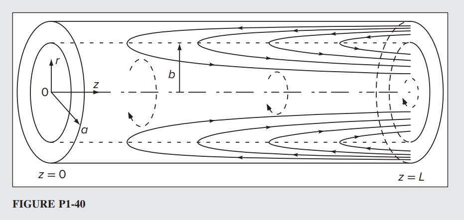
1-40 The Vyas–Majdalani profile, which describes the helical motion of a cyclonic chamber (Vyas and Majdalani 2006), consists of a three-component velocity profile,

where

Here a denotes the radius of the cyclonic chamber, U stands for the average tangential velocity at ra = , and  represents a dimensionless offset swirl parameter that gauges the relative importance of axial and tangential speeds.

(a) Is the flow one-dimensional, two-dimensional, or three-dimensional?

(b) Is the flow steady or unsteady?

(d) Determine the vorticity. Is the flow rotational or irrotational?

(e) Determine the strain rates. What is the sum of the three normal strain rates?

(f) Assuming a circular opening of radius 2 rba == at zL = , calculate the volumetric flow rate by integrating the axial velocity from 0 r = to 2 ra = .

LLC. -28(Ans.)

Hill

) , rzrz

 

2 2 sin r ar vU ra   =−   , a vU r  = , and 2 2 0 2cos;0 z ra zr vU zL aa     =     

(

Vrzveveve

=++ ,

zj rj Zj =1 Zj =2 Zj =3 Zj =4 Zj =5 Solutions Manual for Viscous Fluid Flow 4th Edition White Solutions Manual for Viscous Fluid Flow 4th Edition White

Solution: The velocity varies with respect to the radial distance r from the centerline and axial distance z but it is independent of the angular position

; which corresponds to a typical two-dimensional flow.

(Ans.) Since 0 rz v vv ttt    ===  , the flow is time invariant (steady). (Ans.) Divergence of velocity is ( ) ( ) ( ) ( ) 11 , rz Vrzrvvv rrrz    =++  . ( ) 22 22 22 ,cos0cos0 rr VrzUU aaaa   =−++=   (incompressible) (Ans.) Vorticity is ( ) 111 zrzr rz rv v vvvv veee rzzrrrr          ==−+−+−      Only nonzero component of vorticity is 2 2 32 4 sin z v r Uzr raa     =−=−    (rotational). (Ans.) Only nonzero components of tangential strain rate are 222 111 0 22 r r vv v aaa UUU rrrrrr         =+−=−−=−      (Ans.) Solutions Manual for Viscous Fluid Flow 4th Edition White Solutions Manual for Viscous Fluid Flow 4th Edition White



The sum of the normal strain rate components is

1-41 The Maicke–Majdalani profile, which may be used to describe the motion of an unbounded tornado (Maicke and Majdalani 2009), can be expressed as a simple piecewise approximation for which 0 rz vv== and

where R denotes the radius at which the wind’s angular speed  may be measured and X represents the fraction of the radius R where the free vortex behavior ceases.

(a) Is the flow one-dimensional, two-dimensional, or three-dimensional?

(b) Is the flow steady or unsteady?

(

c) Calculate the divergence of the velocity. Is the flow compressible or incompressible?

(

d) Determine the vorticity. Is the flow rotational or irrotational?

(

e) Determine the strain rates and the shear stresses in each segment of the flow.

(f) What is the limiting value of ( )vr  as 0 r → ?

Solution: The velocity varies with respect to the radial distance r from the centerline and is independent of the axial distance z or of the angular position . This represents a

Copyright 2022 © McGraw Hill LLC. All rights reserved. No reproduction or distribution without the prior consent of McGraw Hill LLC. -3022 22 3232 11 04sin2sin 22 rz zr vv zrzr UrUr zraaaa     =+=−=−     (Ans.)

1 0 rrz rrzz v vvv rrrz        ++=+++=    (Ans.)

volumetric

by ( ) 222 2 2 2 000 2cos2cos2 aa z rr zr QvdAUdraULdaUL aa    ===  ====    (Ans.)

The

flow rate is given

( ) 2 222 2 1ln ; ; rr rXR XXR vr R rXR r       −       =     

Solutions Manual for Viscous Fluid Flow 4th Edition White Solutions Manual for Viscous Fluid Flow 4th Edition White

Then, shear stress is given as follows:

Copyright 2022 © McGraw Hill LLC. All rights reserved. No reproduction or distribution without the prior consent of McGraw Hill LLC. -31typical one-dimensional flow. (Ans.) Since 0 rz v vv ttt    ===  , the flow is time invariant (steady). (Ans.) Divergence of velocity is ( ) ( ) ( ) 11 0 rz vrvvv rrrz    =++=  (incompressible). (Ans.) Vorticity is ( ) 111 zrzr rz rv v vvvv veee rzzrrrr          ==−+−+−      . Only nonzero component of vorticity is ( ) 1 z rv rr   =  . For segment ( rXR  ), 2 222 2 ln z r XXR   =−   (rotational). (Ans.) For segment ( rXR  ), 0 z = (irrotational). (Ans.) Only nonzero component of tangential strain rate is 1 2 r vv rr      =−   . For segment ( rXR  ), 2 r X    =− . (Ans.) For segment ( rXR  ), 2 2 r R r    =− (Ans.)

For segment ( rXR  ), 2 2 r X    =− . (Ans.) For segment ( rXR  ), 2 2 2 r R r    =− . (Ans.) As 0 r → , ( ) 0 vr  → (Ans.) Solutions Manual for Viscous Fluid Flow 4th Edition White Solutions Manual for Viscous Fluid Flow 4th Edition White

1-42 Assuming  to be a scalar and V a vector, evaluate the following quantities:

1-43 Assuming U, V , and W are Cartesian vectors, prove the following identities:

(a) ( ) ( ) ( ) 1 VVVVVV 2 =− (Lamb’s vector identity)

(b) ( ) ( ) 2 VVV=−

(d) ( ) ( )UVWUVW = (mixed vector scalar product)

(e) ( ) ( ) ( ) UVWUWVUVW =− (vector triple product)

(f) ( ) ( ) ( )( ) ( )( )UVUVUUVVUVUV =−

identity)

(b) ( ) ( ) (c) ( )

) (d) ( ) (e) ( )V Solution: 0  = (Ans.) ( ) ( ) 2ijk yzzxxy     =++   (Ans.) ( ) ( ) 2 22 xyz     =++      (Ans.) ( ) 222 222 xyz    =++  (Ans.) ( ) V0= (Ans.)

) 

(

Solutions Manual for Viscous Fluid Flow 4th Edition White Solutions Manual for Viscous Fluid Flow 4th Edition White

(Lagrange’s

(g) ( ) ( ) UVUV2UV −+=

(h) ( ) VVV  =+

(i) ( ) ( ) VVV  =+

(j) ( ) ( ) ( )UVUVUV =+

Solution: ( ) ( ) ( ) ( ) 1 VVVVVVVVVVVV 2 −=−−=   (Ans.)

( ) ( ) ( ) ( ) ( ) 2 VVVVVV −=−−=   (Ans.)

 =−+−+− 

UV VUUV

VUVUVUVUVUVU xyz

zyyzxzzxyxxy yyyy zzzzxxxx xyzxyz

UUVV UUVVUUVV VVVUUU yzzxxyyzzxxy

    =−+−+−−−+−+−        =− (Ans.)

( ) ( ) ( ) ( ) ( ) ( )

UUUVWVWVWVWVWVW

 =−−−+−−−+−−− 

UVWVWUVWVWUVWVWUVWVWUVWVWUVWVW UWUWUWVVVUVUVUVWWW

xyzzyyzxzzxyxxy zxzzxyyxxyxyxxyzzyyzyzyyzxxzzx xxyyzzxyzxxyyzzxyz



(

( ) ( ) ( ) ( ) ( ) UVW UVW zyyzxxzzxyyxxyz zyyzxxzzxyyxxyz VUVUWVUVUWVUVUW VWVWUVWVWUVWVWU =−+−+− =−+−+− = (Ans.) ( ) ( ) ( ) ( ) ( ) ( ) ( ) ( ) ( ) ( ) ( ) ( )( ) ( )( ) ( ) UVW ijkijk

ijkijk UWVU

) ( ) ( )

ijk

 =++−+−+− 

=− ( ) VW(Ans.) ( ) ( ) ( ) ( ) ( ) ( ) ( ) ( ) ( ) ( ) ( ) ( ) ( ) ( ) ( ) ( ) ( ) ( ) 22 2 2222 22 2222 UVUV ijkijk 2 zyyzxzzxyxxyzyyzxzzxyxxy zyyzxzzxyxxy zyyzxzzxyxxyzyyzxzzxyxxy xyzxy UVUVUVUVUVUVUVUVUVUVUVUV UVUVUVUVUVUV UVUVUVUVUVUVUVUVUVUVUVUV UUUVV   =−+−+−−+−+−

=−+−+− =+++++−++  =+++ ( ) ( ) ( )( ) ( )( ) 2 22 UUVVUVUV(Ans.) zxxyyzz VUVUVUV +−++ =− ( ) ( ) ( ) ( ) ( ) ( ) ( ) ( ) ( ) ( ) ( ) UVUV ijkijk 2i2j2k 2UV xxyyzzxxyyzz zyyzxzzxyxxy UVUVUVUVUVUV UVUVUVUVUVUV −+  =−+−+−+++++  =−+−+− = (Ans.) Solutions Manual for Viscous Fluid Flow 4th Edition White Solutions Manual for Viscous Fluid Flow 4th Edition White

=++++−++++

Copyright 2022 © McGraw Hill LLC. All rights reserved. No reproduction or distribution without the prior consent of McGraw Hill LLC. -34( ) ( ) V ijkijk VV xyz y x z y x z xyz VVV xyz V V V xyz V V V VVV xyzxyz            =++++       =++        =+++++    =+ (Ans.) ( ) ( ) ( ) ( ) V ijkijk ijk ijkij xyz yy xx zz yyxx zz zyxz VVV xyz VV VV VV zyxzyx VVVV VV VVVV zyzxxyxyz           =++++       =−+−+−             =−+−+−+−+−+        ( ) ( ) k VV(Ans.) yx VV     =+ ( ) ( ) ( ) ( ) ( ) ( ) UVUV ijkijkijk ijkijk UV xxyyzz xyzxyz yy xx zz xxyyzz UVUVUV VVVUUU xyzxyz UV UV UV xyz UVUVUV xyz +    =+++++++++         =++    =++++    = (Ans.) Solutions Manual for Viscous Fluid Flow 4th Edition White Solutions Manual for Viscous Fluid Flow 4th Edition White