1. Introduction Atmospheric Radar Signal Processing is one field of Signal Processing where there is a lot of scope for development of new and efficient tools for spectrum cleaning, detection and estimation of desired parameters. The echoes received from MST region represents atmospheric background information and is considered to be generated through a random process. Radar signals are very
Signal & Image Processing : An International Journal (SIPIJ) Vol.2, No.3, September 2011 DOI : 10.5121/sipij.2011.2310 101 SIGNAL PROCESSING OF RADAR ECHOES USING WAVELETS AND HILBERT HUANG TRANSFORM N.Padmaja1 Dr.S.Varadarajan2 R.Swathi3 1Associate Professor of ECE Chadalawada Ramanamma Engg College , Tirupati padmaja202@gmail.com 2 Professor of ECE, S.V.University college of Engg, Tirupati. varadasouri@gmail.com 3M.Tech student, IIT Kharagpur rsrsvu@gmail.com Abstract
Keywords: Hilbert-Huang Transformation (HHT), Empirical Mode Decomposition (EMD), Intrinsic mode Functions (IMF), Wavelets, Radar Signals.
Atmospheric Radar Signal Processing is one field of Signal Processing where there is a lot of scope for development of new and efficient tools for spectrum cleaning, detection and estimation of desired parameters. The wavelet transform and HHT (Hilbert-Huang transform) are both signal processing methods. This paper is based on comparing HHT and Wavelet transform applied to Radar signals. Wavelet analysis is one of the most important methods for removing noise and extracting signal from any data. The de-noising application of the wavelets has been used in spectrum cleaning of the atmospheric radar signals. HHT can be used for processing non-stationary and nonlinear signals. HHT is one of the timefrequency analysis techniques which consists of two parts: Empirical Mode Decomposition (EMD) and instantaneous frequency solution. EMD is a numerical sifting process to decompose a signal into its fundamental intrinsic oscillatory modes, namely intrinsic mode functions (IMFs). A series of IMFs can be obtained after the application of EMD. In this paper wavelets and EMD has been applied to the time series data obtained from the mesosphere-stratosphere-troposphere (MST) region near Gadanki, Tirupati for 6 beam directions. The Algorithm is developed and tested using Matlab. Moments were estimated and analysis has brought out improvement in some of the characteristic features like SNR, Doppler width, Noise power of the atmospheric signals. The results showed that the proposed algorithm is efficient for dealing non-linear and non- stationary signals contaminated with noise. The results were compared using ADP (Atmospheric Data Processor) and plotted for validation of the proposed algorithm.
2. Literature Review 2.1. HHT Hilbert-Huang Transform (HHT) can be used for processing non stationary and nonlinear signals.
HHT is one of the time-frequency analysis techniques, which consists of two parts: (a) the EMD, extracting IMFs from the data, and (b) the associated HS, providing information about amplitude , instantaneous phase and frequency.Asthekey part of HHT, EMD is a numerical sifting process to decompose a signal into its fundamental intrinsic oscillatory modes, namely, IMFs allowing IF to be defined.[1] An IMF is defined as a function that must satisfy the following conditions:
Signal 102 weak and buried in noise, hence signal processing methods used for de-noising is necessary.
& Image Processing : An International Journal (SIPIJ) Vol.2, No.3, September 2011
2.2. Wavelet de-noising Wavelet analysis is one of the most important methods for removing noise and extracting signal from any data. The de-noising application of the wavelets has been used in Spectrum cleaning of the atmospheric signals. There are many types of wavelets available. The wavelet families like symlets, coiflets, daubechies, haar etc., have their own specifications like filter coefficients, reconstruction filter coefficients. In the proposed work, Db9, Symlet7, boir3.5 wavelets have been used to eliminate noise embedded in the radar signal. The aim of this study is to investigate the wavelet function that is optimum to identify and de-noise the radar signal. Since Db9 wavelet has found to be optimum in the present case study, it was compared with EMD de-noising. The optimal wavelets are evaluated in term of SNR. In the recent wavelet literature one often encounters the term ‘de-noising’, describing in an informal way various schemes which attempt to reject noise by damping or thresholding in the wavelet domain[10,11]. The threshold of wavelet coefficient has near optimal noise reduction for many classes of signals. Wavelets are used as it provides a whole lot of advantages over FFT. Fourier analysis has a serious drawback. In transforming to the frequency domain, time information is lost. When looking at a Fourier transform of a signal, it is impossible to tell when a particular event took place. Wavelet analysis is capable of revealing aspects of data that other signal analysis technique, aspects like trends,
EMD has found a wide range of applications in signal processing and related fields[6,7]. In this paper wavelet de-noising and EMD has been applied to the radar data and compared in terms SNR.
Most of the approaches aim to enhance Signal to Noise Ratio (SNR) for improving the detection ability. The most common approach is the FFT, which is simplest and straightforward among all the methods. Fourier spectral analysis also requires linearity. However, Fourier Transforms are unsuitable for applications that use nonlinear and non stationary signals. In addition, other technologies, such as wavelet transforms, cannot resolve intra-wave frequency modulation, which occurs in signal systems composed of multiple varying signals. Wavelet transform is widely used as a traditional method to eliminate noise called de-noising. A new data analysis method based on the empirical mode decomposition (EMD) method, which will generate a collection of IMFs is applied to the radar echoes. EMD is a key part of Hilbert-Huang transform (HHT) proposed Norden E. Huang in 1996. HHT can be used for processing non-stationary and nonlinear signals.
(a) In the whole data series, the number of local extrema and the number of zero crossings must either be equal or differ at most by one; (b) At any time, the mean value of the envelope of local maxima and the envelope of local minima must be zero. These conditions guarantee the well-behaved HS [3]. Thus, we can localize any event on the time as well as the frequency axis.
3. Radar data specifications
The MST Radar is located at Gadanki, near Tirupati (13.47°N, 79.18°E). MST radar operates continuously for different type of experimental observations. Here the signal is used on the data recorded corresponds to experiments related to lower atmosphere; i.e. the region of 3.6 km to 20 km. Only sample data is used for analysis to demonstrate the technique. Radar records data for each range gate and the resolution of sample can vary depends on experimental specification. Here the sampling interval corresponds to 150m (1 micro sec.) in space is used and number of samples taken on each range gate is about 512 points. Radar echoes are recorded in 6 beam directions, viz. East, west, zenith x, zenith y, north and south directions. These data are complex in nature and hence the method adopted is complex signal analysis. Each channel (I and Q) is independently treated for all preliminary processes and combined in the final stage while computing Hilbert transforms and FFT. In this paper, EMD has been applied for the data derived from MST regions on two different days and for 6 beam directions. Data set1 is the time series data of good SNR which is recorded during clear weather conditions on 22nd June 2009 and data set II of low SNR is recorded during bad weather on 28th May 2009.
4.2 EMD Algorithm: Given a non-stationary signal x(t) , the EMD algorithm can be summarized into following steps: step(1) Finding the local maxima and minima; then connecting all maxima and minima of signal X(t) using smooth cubic splines to obtain the upper envelop Xu(t) and the lower envelope X l(t) step(2)respectively.Computing
local mean value m1(t) = (Xu(t) + Xl(t))/2 of data X(t), subtracting the mean value from signal X(t) to get the difference: h1(t) = X(t) − m1(t).
EMD is a new signal processing method for analyzing the non-linear and non-stationary signals [2]. EMD is one of the time-frequency analysis techniques which is used for extracting IMFs from the data. EMD is a numerical sifting process to decompose a signal into its fundamental intrinsic oscillatory modes, namely, IMFs allowing IF (Instantaneous Frequency) to be defined. Being different from conventional methods, such as Fourier transform and wavelet transform, EMD has not specified ”bases” and its ”bases” are adaptively produced depending on signal itself. There has better joint time-frequency resolution than Wavelet analysis and the decomposition of signal based on EMD has physically signification [4]. The EMD algorithm has been designed for the time-frequency analysis of real-world signals. Thus, we can localize any event on the time as well as the frequency axis. The decomposition can also be viewed as an expansion of the data in terms of the IMFs. Then, these IMFs, based on and derived from the data, can serve as the basis of that expansion which can be linear or nonlinear as dictated by the data, and it is complete and almost orthogonal. Most important of all, it is adaptive. We focus on using the EMD to radar echoes which can be decomposed into a limited number of intrinsic mode functions. Different thresholds are used to treat intrinsic mode function to achieve de-noising and then compared with the effect of wavelet transform de-noising. EMD is demonstrated to be effective in removing the noise[7].
Signal & Image Processing : An International Journal (SIPIJ) Vol.2, No.3, September 2011 103 breakdown points, discontinuities in higher derivatives, and self-similarity. Wavelet analysis can often compress or de-noise a signal without appreciable degradation.
4. Methodology and Implementation
4.1 Empirical Mode Decomposition: The Sifting Process
(1) In the whole data set, the number of extrema and the number of zero crossings must either be equal or differ at most by one; and (2) at any point, the mean value of the envelope defined by the local maxima and the envelope defined by the local minima is zero We can repeat this sifting procedure k times, until h1k is an IMF. h1(k−1) − m1k = h1k; the result is shown in figure 3(b) after eight siftings. Then, it is designated as c1 = h1k; the first IMF component from the data. As described above, the process is indeed like sifting: to separate the finest local mode from the data first based only on the characteristic time scale. We can separate c1 from the rest of the data by X(t) − c1 = r1 Since the residue, r1, still contains information of longer period components, it is treated as the new data and subjected to the same sifting process as described above. The sifting process is illustrated in figure 2. The sifting process can be stopped by any of the following predetermined criteria: either when the component, cn, or the residue, rn, becomes so small that it is less than the predetermined value of substantial consequence, or when the residue, rn, becomes a monotonic function from which no more IMF can be extracted [8]. By virtue of the IMF definition, the decomposition method can simply use the envelopes defined by the local maxima and minima separately. Therefore, the sifting process should be applied with care.
4.3. INTRINSIC MODE FUNCTIONS
An intrinsic mode function (IMF) is a function that satisfies two conditions:
Signal & Image Processing : An International Journal (SIPIJ) Vol.2, No.3, September 2011 104 step(3) Regarding h1(t) as new data and repeating steps (1) and (2) for k times, h1k(t) = h1(k−1)(t) − m1k(t), where m1k(t) is the local mean value of h1(k−1)(t) and h1k(t). It is terminated until the resulting data satisfies the two conditions of an IMF, defined as c1(t) = h1k. The residual data r1(t) is given by r1(t) = X(t) − c1(t). step(4) Regarding r1(t) as new data and repeating steps (1),(2) and (3) until finding all the IMFs. The sifting procedure is terminated until the nth residue rn(t) becomes less than a predetermined small number or the residue becomes monotonic. step(5) Repeat steps 1 through 4until the residual no longer contains any useful frequency information. The original signal is, of course, equal to the sum of its parts. If we have ‘n’ IMFs and a final residual rn(t), Finally the original signal X(t) can be expressed as follows:
To guarantee that the IMF components retain enough physical sense of both amplitude and frequency modulations, we have to determine a criterion for the sifting process to stop. This can be accomplished by limiting the size of the standard deviation, SD, computed from the two consecutive sifting results. A typical value for SD can be set between 0.2 and 0.3. The process will repeat till the function become monotonic. This can be accomplished by limiting the size of the standard deviation, SD, computed from the two consecutive sifting results as A typical value for SD can be set between 0:2 and 0:3. A SD value of 0:2 for the sifting procedure is a very rigorous limitation for the difference between siftings. The IMF components obtained are designated as C1, the first IMF com ponent from the data, C2, the second IMF component and so on. The nth IMF component is designates as Cn. This technique is attempted to verify the signals received from atmosphere through radar at what extent falls to non-linear and non-stationary in nature. We finally obtain
Formationstartof cubic spline over maxima and minima
105 Figure.1 Flow Chart of Empirical Mode Decomposition
Determination of maxima and minima no
Signal & Image Processing : An International Journal (SIPIJ) Vol.2, No.3, September 2011
Calculateseparatelymeanvalue Mn(t) IsIMFMn no Subtract mean from residue yesStoreIMF Cn monoistic y stop
5.1 Need For Wind Profiles.
Signal & Image Processing : An International Journal (SIPIJ) Vol.2, No.3, September 2011 106 Thus, we achieved a decomposition of the data into n-empirical modes, and a residue, rn, which can be either the mean trend or a constant. -15 -10 -5 0 5 10 15 -0.0500.05amplitude 2( a ) -15 -10 -5 0 5 10 15 -0.0500.05amplitude 2( b ) -15 -10 -5 0 5 10 15 -0.02-0.0400.020.04 Time amplitude 2(C) Figure 2 Illustration of the sifting process (a) The original data (b) the data in thin blue line with the upper and lower envelopes in dot-dashed green and the mean in thick solid line; (c) the difference between the data & mean m1.
Wind profile data is used different domains for research purpose. The MST radar researcher faces many challenges to answer questions and needs to develop expertise in related areas. It is both interesting and useful. The main goal of lower-atmosphere (troposphere + lower stratosphere) research or predictions is to describe and predict the three dimensional structure of the atmosphere at different scales. The wind profiles play an important role. However, temperature and relative humidity information are necessary to provide satisfactory representation of the stability and moisture distribution of the atmosphere. The qualities required for wind data are the robustness, and the availability in all weather conditions; the time and height resolution, and the altitude range required are dependent on the application. The development of wind profilers has given new insights into the behavior of the atmosphere and is useful in various new applications.
5. WIND PROFILES
Vy cos θy +Vz cos θz)2
One of the important applications of the wind profiling is the computation of wind speed. By using the Doppler profiles of the radar returns, wind speed can be calculated at different heights.
For the directions of Zenith-X and Zenith-Y the radar is operated in vertical direction. So the related equation for Doppler frequency is fD = -2Vr/λ λλ λ
V
Vx cos θx
For computing the wind speed, wind profiles for six directions is a must. The wind profiles in North, South, East and West directions with an oblique angle θ are obtained using the algorithms discussed.[13]. The wind profiles in the remaining two Zenith beams are also obtained. If there is a relative motion between the source of the waves and an object encountering the waves, the frequency is measured at the object will be different from that at the source. This is called the Doppler Effect. If the object is approaching the source, the frequency will be higher, if it receding, the frequency will be lower. The amount of frequency change is called the Doppler shift which is directly proportional to the relative radial velocity between the source and the object and inversely proportional to the wavelength. In the case of wind profiling, the source is the wind profiler and the object is the refractive irregularity that scatters the waves. A double Doppler shift is encountered here: one shift as the pulse impinges upon the scattering volume and other as the pulse is scattered back towards the wind profiler.
The –ve sign arises from the fact that positive radial velocities refer to motion away from the radar, which causes the frequency to be lower. From Doppler shift, the radial velocity is given as: Vr = -fDλ/2sin θ
Signal & Image Processing : An International Journal (SIPIJ) Vol.2, No.3, September 2011 107 5.2
The Doppler shift is given as: fD = (-2Vr/λ λλ) sin θ where Vr = radial velocity of the scatters along the beam θ = angle deviated from the vertical direction
Computation of Wind Speed
(V
i
Line of sight component of the wind vector V(Vx,Vy,Vz) is D = V = + Vy +V Where X, Y and Z directions which are aligned to East-West, North-South and Zenith respectively. Applying least square method residual, ε2 = x + and I represents the beam number to satisfy the minimum residual
cos θx
z cos θz
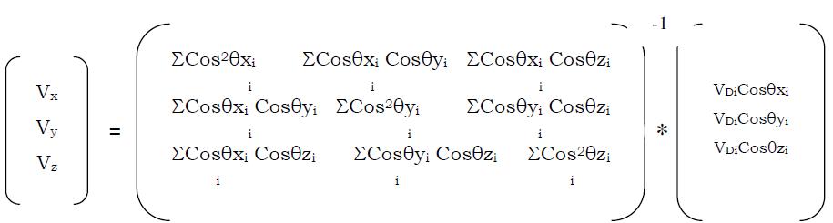
Computation of absolute wind velocity vectors(UVW): After computing the radial velocity for different beam positions, the absolute velocity can be calculated. To compute U, V & W, at least the non coplanar beam radial velocity data is required. If higher number of different beam data are available, then the computation will given an optimum result in the least square method [14].
cos θy
Signal & Image Processing : An International Journal (SIPIJ) Vol.2, No.3, September 2011 108 ∂ε2 /∂Vk = 0 k corresponding to X, Y, and Z leads to Zonal velocity(U): Zonal velocity=(Radial velocity in East direction + Radial velocity in west direction)/2 U=(VrE+Vrw)/2 Meridional velocity)V): Meridional velocity = (Radial velocity in North direction + Radial velocity in south direction)/2 V = (NrN+VrS)/2 Vertical velocity: Vertical velocity = (Radial velocity in Zenith X direction + Radial velocity in Zenith Y direction)/2 W = (VrZ-x+VrZ-y)/2 Using the zonal velocity, meridional velocity and wind speed can be computed as follows: The magnitude of wind speed = 5. Results and discussion EMD algorithm has been applied to all the 6 beams viz. – east, west, zenith x, zenith y, north and south beams. Sifting process has been illustrated in figure 2 for the 1st range bin of the data of 22 June 2009. The shifting process is illustrated for 1st IMF only. The Intrinsic mode functions obtained by applying EMD on two sets of the atmospheric data is shown in figures 4 and 6. Similarly imf’s are obtained for all the beams and for different range bins. The original Doppler profile using FFT is shown figure 5 for beam 1(East beam). Similar results have been obtained for all the 6 beams. Figure 5 is the comparison of original & reconstructed signal (22 June 2009).
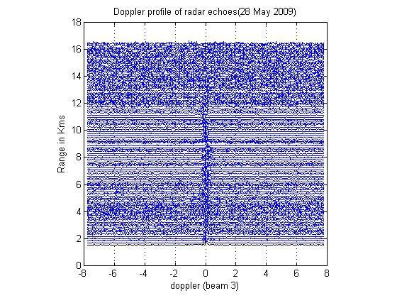
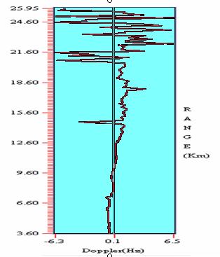
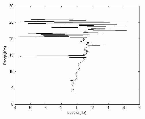
Signal & Image Processing : An International Journal (SIPIJ) Vol.2, No.3, September 2011 109 Figure. 3 (a) Doppler profile radar data of good SNR (22 June 2009) (b) Doppler profile radar data of low SNR (28 May 2009 ) Figure. 4 Intrinsic mode functions of East Beam for 10th Range bin (22 June 2009)
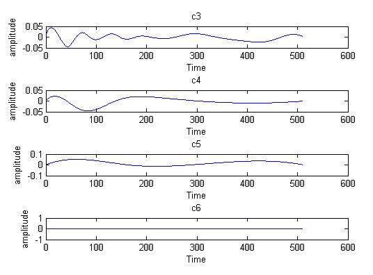
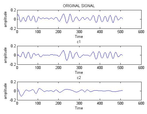
Signal & Image Processing : An International Journal (SIPIJ) Vol.2, No.3, September 2011 110 Figure 5. comparison of original & reconstructed signal (22 June 2009) Figure 6 Intrinsic mode functions of Zenith Y Beam for 90th Range bin (28 May 2009)
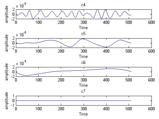
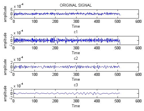
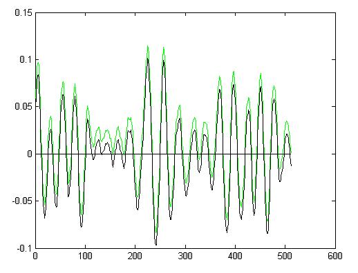
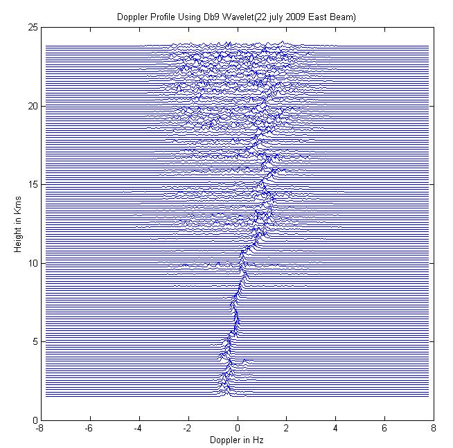
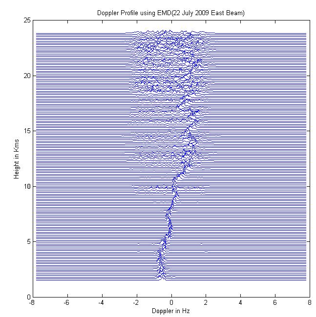
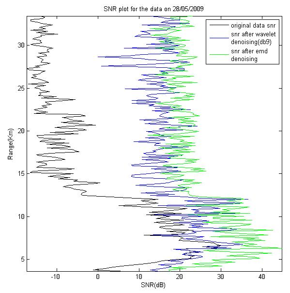
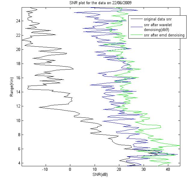
Fig.4 shows the IMFs extracted from radar data for 10th range bin with better SNR during clear weather conditions (22 June2009) and Fig.6 shows the IMFs extracted after applying the EMD algorithm to the radar data of low SNR during cloudy and noisy weather (28 May 2009). ‘C1’ is the first IMF component from the data. ‘C2’ is the second IMF component and so on. Figur 7 is the Doppler profile plotted using db9 wavelet and emd. For validation of results, SNR has been plotted for the two data sets using Db9 wavelet and EMD and further compared with ADP (Atmospheric Data Processor). The results showed an improvement of SNR when EMD is used compared to wavelet de-noising using Db9.
Fig 7 Doppler profile of east beam of 22 July 2009 using Db9 wavelet de-noising and EMD.
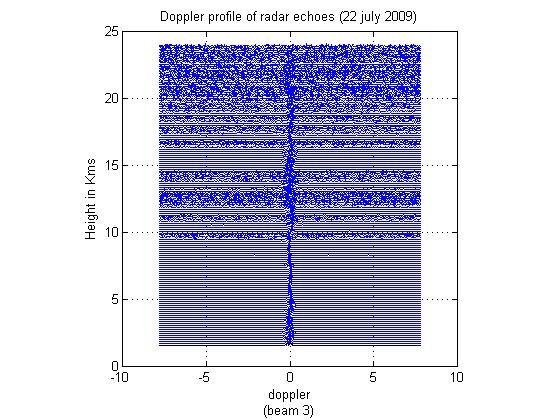
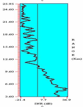
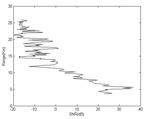
The first few IMFs, in Fig. 4 and 5 correspond to the high-frequency noise embedded in the data. It is illustrated from Figure 4 that the EMD resulted in 7 imf components (c1–c8) corresponding to data collected for low SNR data during noisy weather. Where as for clear weather data, the application of the EMD algorithm resulted in 6 imf components (c1-c6) due to better SNR. For verification and comparison, FFT has also been applied on the same data and the Doppler profile has been plotted. It is evident from the Doppler profile( figures 3a & 3b) that the data on 28 May is contaminated with noise and the data on 22 June is better. The Doppler profile is very clearly visible upto 10Kms for data set I and not so clear above 10 Kms. This is due the low SNR of the echo signals at greater heights. The doppler profile for data set II is not so clear even below 10 Kms. This is due the low SNR of the echo signals due to bad weather conditions and clutter. Figures 8(a) & 8(b) are the SNR Plots of the two sets of Radar Data. From the SNR plots , an average improvement of about 6 to 10 db in SNR is obtained using Emd de-noising compared to wavelet de-noising. Large set of data has been used for validating the performance of the algorithm. In all cases it is observed that EMD out performs the wavelets in extracting information. For all the beam directions, the results obtained were in correlation.
111
Signal & Image Processing : An International Journal (SIPIJ) Vol.2, No.3, September 2011
Implications
Signal & Image Processing : An International Journal (SIPIJ) Vol.2, No.3, September 2011 112 Figure 8 (a) SNR Plot of Radar Data (22 June 2009) Figure 8 (b) SNR Plot of Radar Data (28 May 2009)
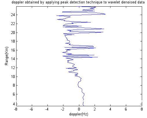
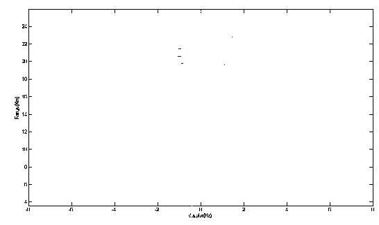
(b) Mean Doppler height profile using level 1 db9 wavelet denoising.
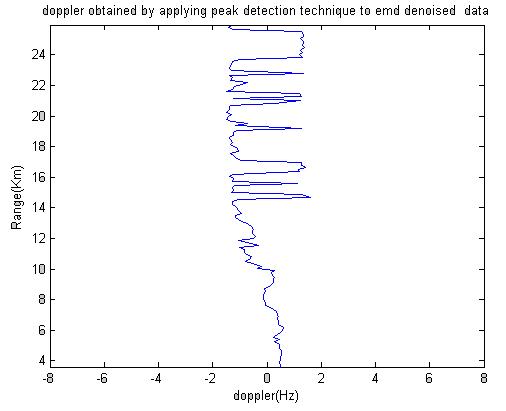
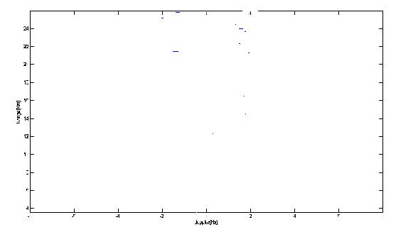
(c) Mean Doppler height profile using emd denoising.
Signal & Image Processing : An International Journal (SIPIJ) Vol.2, No.3, September 2011 113
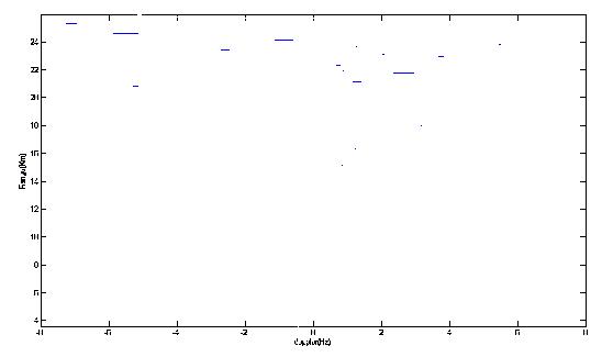
Figure10 (a) Mean Doppler height profile extracted from the spectrum using Single peak detection method (28 May 2009)
(b) Mean Doppler height profile extracted using level 1 b9 wavelet denoising.
(c) Mean Doppler height profile extracted using emd denoising.
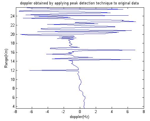
Figure 9(a) Mean Doppler height profile extracted from the spectrum using single peak detection method (22 June 2009)
Signal & Image Processing : An International Journal (SIPIJ) Vol.2, No.3, September 2011 114 Figure 11. Doppler computed for east beam data using ADP and peak detection technique Figure 12. SNR computed for east beam data using ADP and peak detection technique
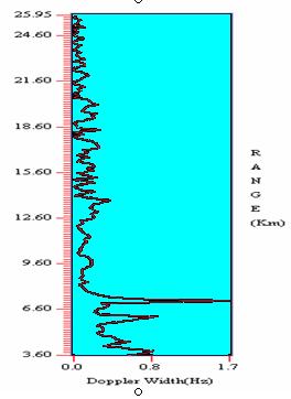
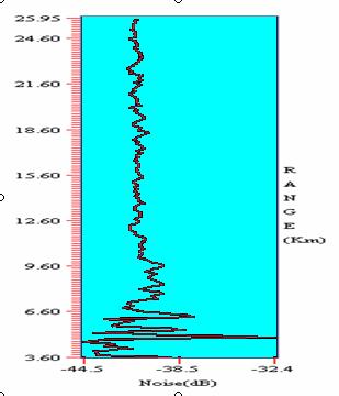
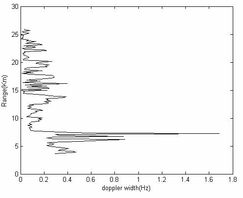
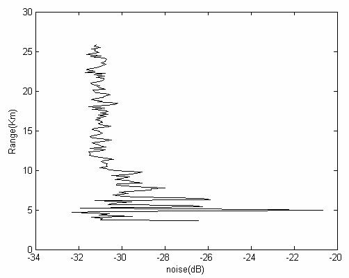
Signal & Image Processing : An International Journal (SIPIJ) Vol.2, No.3, September 2011 115 Figure 13 Doppler width computed for east beam data using ADP & Matlab Figure 14 Noise power computed for east beam data using ADP & Matlab
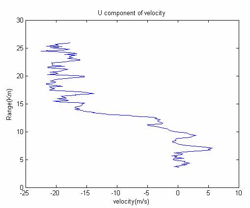
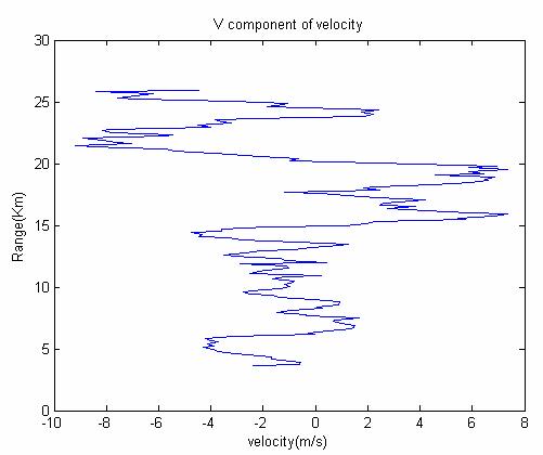
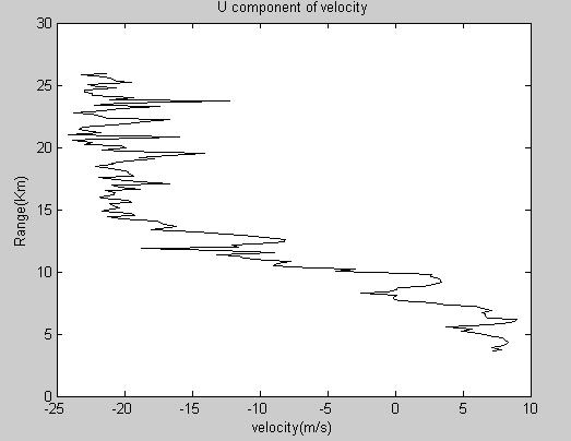
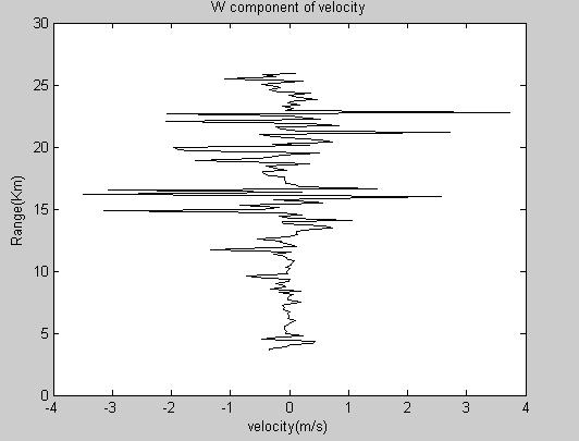
Signal & Image Processing : An International Journal (SIPIJ) Vol.2, No.3, September 2011 116 Figure 15(a) U component using FFT & EMD Figure 15(b) V component using FFT & EMD

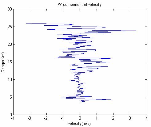
Signal & Image Processing : An International Journal (SIPIJ) Vol.2, No.3, September 2011 117
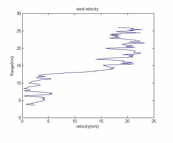
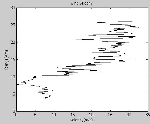
Figure 15(c) W component using FFT & EMD Figures 9 and 10 are the mean doppler height profiles extracted from the spectrum using single peak detection method for both the radar data sets viz. 22 June 2009 & 28 May 2009 using level 1 db9 wavelet denoising & emd denoising. For validation of the proposed algorithm, the results were compared with ADP. Figure 11 shows the Doppler computed for east beam data using ADP and FFT using peak detection technique. Figure 13 shows the Doppler width computed for east beam data using ADP & FFT. Figure 14 Noise level computed for east beam data using ADP & FigureFFT 15(a), 15(b) & 15(c) are the plots of U,V,W components using ADP & FFT. Figure 16 is the Wind velocity plot using ADP & FFT. From the above figures, the results were in correlation with the standard ADP software used by the scientists at gadanki. Figure 16 Wind velocity computed using FFT & EMD
[5] Naveed ur Rehman, Student Member, IEEE, and Danilo P. Mandic, Senior Member, IEEE [6] Flandrin P, Rilling G, Goncalves P., “Empirical mode decomposition as a filter bank”. IEEE Signal ProcessingLetters, Feb. 2004, Vol. 11, Issue 2, Part 1, pp: 112–114.
2) Because the basic functions which are extracted from original data and base on residue of the last filtering are alterable in HHT, the EMD is adaptive. But the basic function of wavelet transform is given, and the effect of de-noising is affected greatly by the choice of basic wavelet. It is demonstrated that HHT techniques are able to resolve frequency components with finer resolution. This is one of the important properties of this method and applied to non linear and non stationary signals. Large set of data has been used for validating the performance of the algorithm. In all cases it is observed that HHT out performs the wavelets in extracting information. For all the beam directions, the results obtained were in correlation. These results in help in classifying the signals received from atmosphere using remote sensing radars. This is a promising technique for enhancing the capability of detection of signals with finer details. All examples presented here testify to the usefulness of this new method. The analysis is further extended to time frequency analysis of the atmospheric signals to HS (Hilbert Spectrum). Once the IMFs are obtained, instantaneous frequency of each IMFs can be determined by Hilbert transform Also Moments, and various parameters of radar data are estimated, analyzed and compared with ADP and plotted.
[6] N.E Huang, S.R.Long, and Z shen, “A new view of nonlinear water waves: The Hilbert spectrum”, Annu.Rev. Fluid Mech, 1999.Vol.31, pp. 417-457.
7. References [1] Norden E. Huang, Z. Shen, and S. R. Long, M.L.Wu, E. H. Shih, Q. Zheng, C. C. Tung, and H. H. Liu,“The Empirical Mode Decomposition and the Hilbert Spectrum for Nonlinear and NonstationaryTime Series Analysis,” Proceedings of the Royal Society of London A, (1998) vol. 454, pp 903-995 [2] Z. Wu and N. E. Huang, “A study of the characteristics of white noise using the empirical modedecomposition method”. Proc. Roy. Soc London A, 2004, Vol. 460, pp. 1597-1611.
Signal & Image Processing : An International Journal (SIPIJ) Vol.2, No.3, September 2011 118 6. Conclusion In this paper, different thresholds are used to treat intrinsic mode function to achieve de-noising and then compared with the effect of wavelet transform de-noising. Hilbert-Huang Transform is demonstrated to be effective in removing the noise embedded in radar echoes. To compare results, wavelet transform and HHT methods are used to deal with the same data to show the effect of de-noising. We add up all the new IMFs which are treated with threshold, and reconstruction of radar signal is done. We can get the following conclusions by comparison:
1) Both HHT and wavelet transform can be used to analyze non stationary signal and can achieve the desired effect of de-noising.
[3] Z.K. Peng, Peter W. Tseb, F.L. Chu. “An improved Hilbert–Huang transform and its application in Vibration signal analysis”. Journal of Sound and Vibration 286 (2005) 187–205 [4] Dejie Yu, Junsheng Cheng, Yu Yang. “Empirical Mode Decomposition for Trivariate Signals” IEEE transactions on signal processing, vol. 58, no. 3, March 2010.
[8] R. Gabriel and F. Patrick. “ The Empirical Mode Decomposition Answers”. IEEE Transactions on Signal Processing, vol. 56, No. 1, 2008.
Signal & Image Processing : An International Journal (SIPIJ) Vol.2, No.3, September 2011
Dr S.Varadarajan is working as Professor in Department of Electronics and Communication Engineering, S V University College of Engineering, Tirupati, India. He received Ph.D (ECE) from S V University, Tirupati in 2003. He has 25 years of teaching experience. He has widely published and presented research and technical papers in International Journals, National Journals & conferences. His areas of interests include Signal & Image Processing, Digital Communications. Systems. He is a fellow member of IETE. He chaired and served as reviewer of number of international conferences and is a member of editorial board of International journals. He visited USA, UK.
[12] Norden E. Huang, Man-Li Wu, Wendong Qu, Steven R. Long.Applications of Hilbert–Huang transform to non-Stationary Financial time series analysis. Appl. Stochastic Models Bus. Ind., 2003; 19:245–268 [13] Rotteger. J and M.F.Larsen , UHF/VHF Radar techniques for atmospheric research and Wind Profiler applications.
[11] Dong Yinfeng, Li Yingmin, Xiao Mingkui, Lai Ming, “Analysis of earthquake ground motions using an Improved Hilbert–Huang transform”. Soil Dynamics and Earthquake Engineering, Jan. 2008, Vol. 28,Issue 1, pp:7-19.
[9] Z. K. Penga, Peter W. Tse, F. L. Chu, “A comparison study of improved Hilbert–Huang transform and Wavelet transform: Application to fault diagnosis for rolling bearing,” Mechanical Systems and Signal Processing, pp. 974–988, 2005.
[10] Yuan Li. ”Wavelet Analysis for Change Points and Nonlinear Wavelet Estimates in Time Series.” Beijing: China Statistics Press, 2001.
[14] Doviak.R.J and Zrnic.D.S , Doppler Radar and Weather observations, Academic Press, London 1984 Authors Mrs N. Padmaja received B E (ECE) from University of Mumbai, India in 1998 and M Tech (Communication Systems) from S V University College of Engineering, Tirupati in 2003. She is pursuing Ph.D. from S V University, Tirupati . Currently she is working as Associate Professor, Dept of Electronics and Communication Engg., C R Engineering College, Renigunta Road, Tiupathi, India. She published and presented 7 technical papers in various in International Journals and conferences. She is a life member of ISTE and IETE. Her areas of interests include Signal Processing, Comm Systems and Computer Communication Networks.
Ms R.Swathi is presently pursuing M.Tech in IIT, Kharagpur. She received her B.Tech degree from S.V.University of Engineering , Tirupati. Her areas of interests include Signal and Image processing and Digital communications.
119 [7] Wang Chun, Peng Dong-ling, “The Hilbert-Huang Transform and Its Application on Signal Denoising”, China Journal of Scientific Instrument, 2004, Vol.25,no.4, pp. 42-45.