Evaluating the Accuracy of a Linear Regression Model in Predicting the Dissolution of Tablets Based

EVALUATING THE ACCURACY OF A LINEAR REGRESSION MODEL IN PREDICTING THE DISSOLUTION OF TABLETS BASED ON RAMAN MAPS

Gábor Knyihár, Kristóf Csorba and Hassan Charaf

Department of Automation and Applied Informatics, Faculty of Electrical Engineering and Informatics, Budapest University of Technology and Economics, Budapest, Hungary

ABSTRACT

Investigation of the dissolution of tablets is an important area of pharmaceutical research. Such research aims to predict the dissolution process as accurately as possible without destroying the tablets. Several methods have been published that can estimate dissolution with approximate accuracy, but they are primarily complex learning algorithms that are time-consuming and require many samples to train. This article seeks to answer whether these complex models are necessary or whether a similar result can be achieved with the help of more straightforward methods. Therefore, during this work, a simpler linear regression model was created and analysed its effectiveness in estimating the dissolution curves. The investigation concluded that the results are not as accurate as in the case of more complex methods, but the model is more robust and can be used in the case of fewer samples. Thus, by further developing these and combining the methods, we can achieve better results in the future.

KEYWORDS

Raman spectroscopy, Dissolution curve, Linear regression, Principal Component Analysis

1. INTRODUCTION

One of the much-studied areas of pharmacy is the dissolution test of sustained-release tablets. The purpose of such a tablet is not to dissolve immediately after entering the body but to continuously distribute the amount of active ingredient (API) determined by pharmacists into the body for a specific period. The dissolution of tablets is usually characterised by dissolution curves, which show the percentage of the dissolved API in the proportion of the time. Today, the most reliable and frequently used method for determining the dissolution curve is a physical measurement, during which the tablet is placed in a liquid similar to stomach acid, and the amount of dissolved API is measured [1]. The method gives accurate results, but its major drawback is that it is incredibly time-consuming (it can take up to 12 or 24 hours to dissolve one tablet). Furthermore, it destroys the only tablet whose dissolution process is known.

For this reason, many types of research aim to estimate the progress of dissolution as simply, quickly and, most importantly, non-destructively as possible. Many try to estimate the dissolution curve using modern artificial intelligence methods [2] [3] [4] [5]. The crushing strength of tablets, compression force applied during production, and Raman and near-infrared (NIR) spectra are commonly used as inputs [6]. Other papers try to solve the problem

analytically [7], but the dissolution process can depend on many parameters, making these models complex.

This article examines the accuracy of a more straightforward linear regression (LR) model compared to more complex neural network methods. Galata et al. [5] present two methods for estimating the dissolution curve, which they refer to as discretisation (DI) and wavelet analysis (WA) methods. In this article, the same dataset is used as the author of the reference article, so the obtained results can be directly compared.

Raman maps of the tablets were used as input. In pharmaceutical research, light-based spectral analysis methods are often used, among which near-infrared and Raman spectroscopy are widespread [8]. With the latter, we can take pictures of a small surface, based on which the ratio and arrangement of the elements that make up the surface can be determined without destroying it. While preparing the Raman map, a particular device, the Raman spectrometer, illuminates the tablet's surface at each grid point with laser light and records the variations in the wavelength of the reflected light [9] [10]. From the obtained spectra, compared with the reference spectra of the pure components, the percentage occurrence of the components in each point can be determined using the classical least squares (CLS) method after the required preprocessing steps [11] [12].

With Raman maps, the goal is to investigate the tablet's composition since these tablets contain a hydrophilic matrix that directly affects the time course of dissolution. A hydrophilic matrix is homogeneous dispersion of molecules in which one or more components can be interpreted as hydrophilic polymers. These hydrophilic polymers are cellulose derivatives that swell in contact with water, slow the API's outflow, and hold the tablet together. Hence, the wetting of the internal parts occurs much later [7]. For this reason, we look for the amount and location of this material in Raman maps, as this provides the most information about the dissolution process [5].

2. THE USED DATA AND METHODS

The following sections contain a description of the data used and a detailed explanation of the methods.

2.1. The Tested Tablets

The measurement results published by Galata et al. [5] were used for the calculations. The dataset contains information on 28 tablets, of which 18 were used for training and 10 for validation. Each tablet consists of 4 components: the API (drotaverin, DR), the hydrophilic matrix polymer (hydroxypropyl methylcellulose, HPMC), the filler (lactose) and the lubricant (magnesium stearate, MgSt). Their proportions are presented in Table 1. The factor that most influence the tablets' dissolution is the matrix polymer's ratio and particle size. So the dataset distinguishes between small (<45 µm) and large (>125 µm) HPMC tablets and varies the proportion of HPMC. The training dataset contains 6 different compositions (3 tablets each), while the validation data set contains 10 different compositions (1 tablet each).

Signal & Image Processing: An International Journal (SIPIJ) Vol.14, No.1, February 2023

Table 1. The parameters of investigated tablets [5]

2.2. Raman Maps

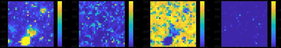
There are 4 Raman maps available for each tablet, 1 for each component. These were made on a small 1.2×1.2 mm2 part of the tablet surface with a step interval of 40 µm, in a total of 31×31=961 points. Each point on the map shows the proportion of the given component in the tablet. Figure 1 shows an example of the Raman maps available for tablets.

It is essential to highlight here that the Raman maps that have already been evaluated were used during the work, i.e., those that show the proportions of the components that make up the tablets. The recording, preprocessing, and evaluation of the spectra performed by Galata et al. [5] was carried out and made available to us in this form. Hence, its discussion is not part of this description.

2.3. Dissolution Curves

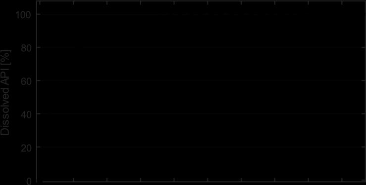
In addition to the Raman maps, the dissolution curve of each tablet is available. The curves give the concentration of the dissolved API at a total of 38 points in time. These points are 0, 2, 5, 10, 15, 30, 45 and 60 minutes from the beginning of the measurement and every 30 minutes after that up to 960 minutes. An example of this is shown in Figure 2.

2.4. Software

To perform the calculations, Matlab 2021b (v9.11) software developed by Mathworks supplemented with the Image Processing Toolbox (v11.4) and the Statistics and Machine Learning Toolbox (v12.2) was used.

2.5. Processing of Raman Maps

Only the HPMC ratio of the tablets was considered during the work since the dissolution process depends mainly on this component. The HPMC map was discretised as a first step by assigning a group denoted by numbers between 1-10 to each pixel. The assignment is given by the Equation 1.

, where��∈[0,1]

Figure 1. Raman maps for the tablet T10S1. The first map shows the ratio of DR, the second of HPMC, the third of Lactose, and the fourth of MgSt on the tablet's surface. The �� and �� axes of the maps show the distance relative to the centre in µm.

Figure 2. Dissolution curve for the T10S1 tablet. The bottom axis shows the time from the beginning of the measurement in minutes, and the left axis shows the percentage of the dissolved API.

Signal & Image Processing: An International Journal (SIPIJ) Vol.14, No.1, February 2023

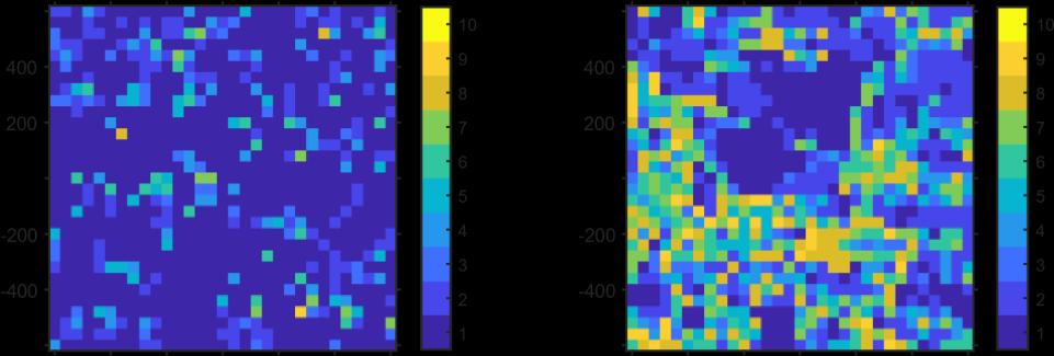
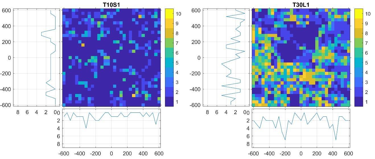
So, for example, the pixels whose value is greater than 0 and less than or equal to 0.1 belong to Group 1. The individual groups are meant to symbolise connected HPMC parts, and the higher the value of each group, the higher the proportion of HPMC found there. Figure 3 shows an example of two discretised maps with different HPMC content.

The figure clearly shows that in the case of the T30L1 sample, which contains a higher percentage of HPMC, significantly more regions can be found that belong to the groups denoted with larger numbers.

In order to characterise the regions with different HPMC content, we counted the number of each group in each row and column. For example, in the first column of the T10S1 sample shown in Figure 3, there are 21 1s, three 2s, five 3s, … and so on. Thus, we got 2×31=62 values for the 10 groups, i.e., a total of 620 values. After calculating the parameters for the maps, we get a matrix of size 18×620, where the parameters belonging to one tablet are located in each row of the matrix. To make this matrix a manageable size and eliminate unnecessary parameters, the dataset was reduced to 17 principal components (PC) using principal component analysis (PCA). After that, the input became 18×17 in size.

2.6. Creation of a Linear Regression Model for the Prediction of Dissolution Curves

In order to create the LR model, the set of parameters described in the previous chapter was used as input. For the output, the values of the reference dissolution curves were arranged in an 18×38 matrix. In the matrix, each row belongs to a tablet, and each column belongs to a particular time moment. Then, using the method of least squares, the �� matrix was searched that balances the Equation 2 with the smallest possible �� error. �� is the parameter matrix used as input, and �� is the dissolution curve matrix used as output.

After that, the model was validated. The input parameter matrix was calculated for the validation maps, as in the training set.

The only difference was that the transformation obtained during training was used instead of PCA, and the input parameters were transformed into the same PC as the training set. The dissolution curves were determined using a matrix multiplication between the received inputs and the model defined during training. The results were then bounded using the assumption that the dissolution values could only be interpreted between 0-100, so the values that did not fit into this range were replaced by the limit values of the range.

Figure 3. Discretised HPMC maps for T10S1 and T30L1 tablets. The �� and �� axes of the maps show the distance relative to the centre in µm, and the colours symbolise the individual groups between 1 and 10.

2.7. Evaluation of the Accuracy of the Estimated Curves

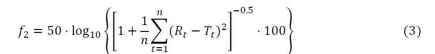
The ��2 value described by Duan, Riviere and Marroum [13] was used to compare the calculated and measured dissolution curves, a commonly used metric in the field. The value is given according to the Equation (3), where ���� and ����are the calculated and measured dissolution values at the time of ��, and �� is the number of time moments.

The ��2value is 100 if the two analysed curves are equivalent and less than 100 if they differ. So the goal is to make the ��2 value as large as possible.

3. RESULTS

3.1. Examination of Raman Maps

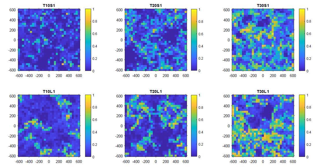
For effective dissolution prediction, it is crucial to characterise the tablets with the appropriate parameters. In the case of the investigated tablets, such a parameter is the proportion and particle size of HPMC. If the tablets with different compositions are examined (Figure 4), it is visible that there are differences between the maps. The more significant HPMC content is represented by more, higher-value pixels, and the larger particle size appears in their larger connected areas.

During the discretisation of the maps, the goal was to manage the values of the maps efficiently. Several divisions were tried, but the best results were obtained when the maps were discretised into 10 groups. This way, a manageable number of groups and parameters were created, but the data's information content remained. There were several options during the creation of the

Figure 4. Comparison of HPMC maps of tablets with different compositions. The upper row contains the small and the lower row the large particle size samples with 10, 20 and 30% HPMC content from left to right. Every map shows the HPMC content of tablet number 1 from each composition. The �� and �� axes of the maps show the distance relative to the centre in µm.

parameter set. Galata et al. [5] used a different metric, but the linear models could not give outstanding results with them, so it was necessary to create a new metric.

The aim during the implementation of this metric was to make the outcome include not only the amount of HPMC but also provide some information about their arrangement. The best results were obtained when the described row and column calculation was used, which resulted in a notable amount of parameters. The latter method can only be used if the maps are previously discretised. By reducing the number of groups used during discretisation, we could get fewer parameters, but we would also significantly distort the map's values. With the help of row-byrow and column-by-column summarisation, we can extract more information from the maps. First, the sum of the obtained values will be proportional to the HPMC content. Second, if the values are interpreted as a curve, then the shape of it also gives information about the arrangement of the HPMC grains. For example, slight differences between the values mean an even distribution of HPMC, while jumpy values indicate areas of higher concentration. Take samples T10S1 and T30L1 as an example (Figure 5). In order to be evident, the figure only shows the calculated curves for group 5. It can be seen that in the case of sample T30L1, which contains more HPMC, the values are not only higher, but given that this is a sample with a large particle size, we also find higher continuous values. For sample T10S1, which contains less HPMC, the curve shows many more values close to 0, and only a few outliers can be seen.

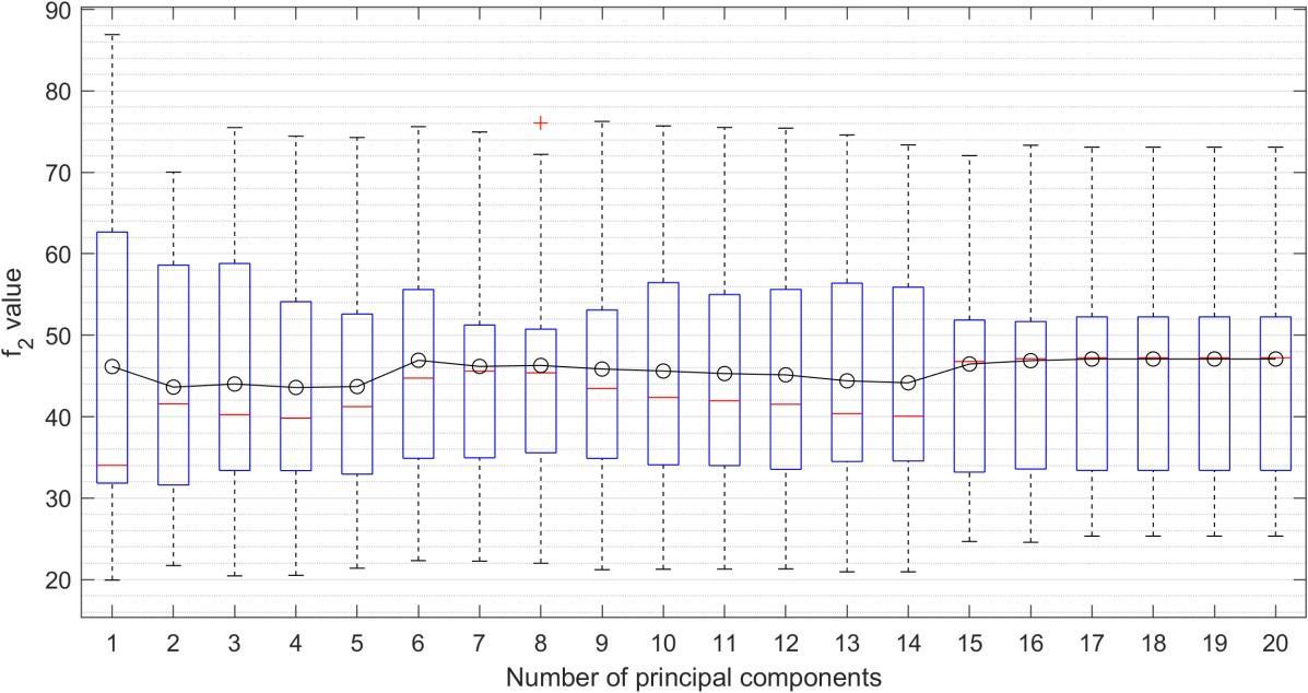
The obtained data set can be divided using PCA into 17 independent variables. We tried several combinations of principal components, but the best results were obtained when the number of PC was chosen to be 17 or more. Similar good results can be achieved by 6 PC, but as you can see on the boxplot (Figure 6), the model is more robust with 17 PCs.

Figure 5. Visualisation of row-by-row and col-by-col summarisation for T10S1 and T30L1 samples. The plots on the left and bottom sides of the maps show the number of pixels with the value 5 in the respective rows and columns.

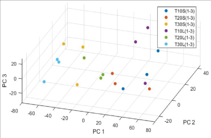
Here, the large number of PCs follows from a large number of parameters. The first few main components have the most significant influence, while the others help to refine the results. By plotting the first three of these in space (Figure 7), it can be concluded that the HPMC content correlates with the first PC and that the individual tablets belonging to them are located close to each other, which may contain information about the different compositions.

3.2. Accuracy of Dissolution Prediction

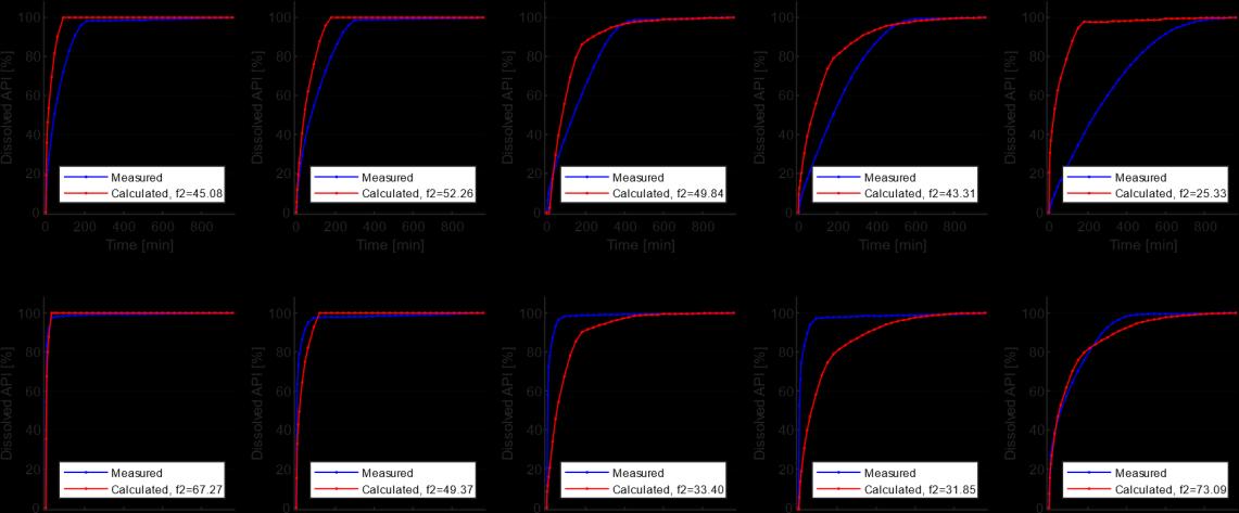
Based on the obtained LR model, the dissolution curves for the 10 validation maps were calculated and compared with the measured curves by determining the already described ��2 value for each sample (Figure 8). The best-performing model gave an average of 47.08 for the ��2 value, which is a relatively good result.

Figure 6. The change in ��2 values based on the principal component number is represented on a boxplot. The black circles show the average values for the respective PC number.

Figure 7. Representation of the parameters of the training set along the first 3 PC. The 3 axes correspond to the first 3 PC. Dots of the same colour belong to tablets of the same composition.

The obtained results were compared with the results of Galata et al. [5] (Table 2). It is visible that the LR model needs to be revised to the DI and WA methods reported in the article. However, the LR method is significantly more straightforward and robust, as all the methods explained in the article use a neural network, the training and calibration of which is a lengthy and complex procedure.

Furthermore, if validation samples are analysed individually, in some cases, the LR model gives better results than the ones reported in the reference article. Consequently, it may be possible to achieve better results by combining these methods.

4. CONCLUSIONS

This article analysed a linear regression model's accuracy in predicting tablets' dissolution curves based on their Raman map. The results showed that, still, the model could not achieve better results in general than the methods that do the same with the help of a neural network. However,

Figure 8. The calculated dissolution curves of the validation dataset compared to the measured values. The bottom axes of the figures show the time from the beginning of the measurement in minutes, and the left axes show the percentage of the dissolved API.

Table 2. Comparison of the ��2 value of the DI and WA methods [5] with the results of the LR method.

Signal & Image Processing: An International Journal (SIPIJ) Vol.14, No.1, February 2023

the method is significantly more robust and performs better in some cases. This result indicates a strong correlation between the metrics determined based on the Raman maps and the dissolution. Compared to methods using neural networks, the advantage of the linear regression model is that it can be used with a smaller number of samples, and the characterisation of the relationships between individual parameters is much more transparent. The linear one is the simplest among the regression models, so there are still many opportunities for further development to achieve better results in dissolution prediction by examining different models. Furthermore, it would be worth investigating whether linear regression could be used as a supporting method in addition to a neural network and what kind of increase in accuracy could be achieved by combining the two methods.

ACKNOWLEDGEMENTS

The work presented in this paper has been carried out in the frame of project no. 2019-1.1.1PIACIKFI-2019-00263, which has been implemented with the support provided from the National Research, Development and Innovation Fund of Hungary, financed under the 2019-1.1. funding scheme.

REFERENCES

[1] J. B. Dressman and J. Krämer, Pharmaceutical dissolution testing, Taylor & Francis Boca Raton, FL:, 2005.

[2] B. Nagy, D. Petra, D. L. Galata, B. Démuth, E. Borbás, G. Marosi, Z. K. Nagy and A. Farkas, "Application of artificial neural networks for Process Analytical Technology-based dissolution testing," International journal of pharmaceutics, vol. 567, p. 118464, 2019.

[3] D. L. Galata, A. Farkas, Z. Könyves, L. A. Mészáros, E. Szabó, I. Csontos, A. Pálos, G. Marosi, Z. K. Nagy and B. Nagy, "Fast, Spectroscopy-Based Prediction of In Vitro Dissolution Profile of Extended Release Tablets Using Artificial Neural Networks," Pharmaceutics, vol. 11, p. 400, 2019.

[4] D. L. Galata, Z. Könyves, B. Nagy, M. Novák, L. A. Mészáros, E. Szabó, A. Farkas, G. Marosi and Z. K. Nagy, "Real-time release testing of dissolution based on surrogate models developed by machine learning algorithms using NIR spectra, compression force and particle size distribution as input data," International Journal of Pharmaceutics, vol. 597, p. 120338, 2021.

[5] D. L. Galata, B. Zsiros, L. A. Mészáros, B. Nagy, E. Szabó, A. Farkas and Z. K. Nagy, "Raman mapping-based non-destructive dissolution prediction of sustained-release tablets," Journal of Pharmaceutical and Biomedical Analysis, vol. 212, p. 114661, 2022.

[6] K. Yekpe, N. Abatzoglou, B. Bataille, R. Gosselin, T. Sharkawi, J.-S. Simard and A. Cournoyer, "Predicting the dissolution behavior of pharmaceutical tablets with NIR chemical imaging," International journal of pharmaceutics, vol. 486, p. 242–251, 2015.

[7] C. Maderuelo, A. Zarzuelo and J. M. Lanao, "Critical factors in the release of drugs from sustained release hydrophilic matrices," Journal of controlled release, vol. 154, p. 2

19, 2011.

[8] K. C. Gordon and C. M. McGoverin, "Raman mapping of pharmaceuticals," International journal of pharmaceutics, vol. 417, p. 151–162, 2011.

[9] J. R. Ferraro, Introductory raman spectroscopy, Elsevier, 2003.

[10] F. A. Miller and G. B. Kauffman, "CV Raman and the discovery of the Raman effect," Journal of Chemical Education, vol. 66, p. 795, 1989.

[11] J. F. Kauffman, M. Dellibovi and C. R. Cunningham, "Raman spectroscopy of coated pharmaceutical tablets and physical models for multivariate calibration to tablet coating thickness," Journal of pharmaceutical and biomedical analysis, vol. 43, p. 39–48, 2007.

Signal & Image Processing: An International Journal (SIPIJ) Vol.14, No.1, February 2023

[12] L. A. Mészáros, D. L. Galata, L. Madarász, Á. Köte, K. Csorba, Á. Z. Dávid, A. Domokos, E. Szabó, B. Nagy, G. Marosi and others, "Digital UV/VIS imaging: A rapid PAT tool for crushing strength, drug content and particle size distribution determination in tablets," International Journal of Pharmaceutics, p. 119174, 2020.

[13] J. Z. Duan, K. Riviere and P. Marroum, "In vivo bioequivalence and in vitro similarity factor (f2) for dissolution profile comparisons of extended release formulations: how and when do they match?," Pharmaceutical research, vol. 28, p. 1144–1156, 2011.