Maxwell’s Theory of Electromagnetism

Samuel Rayner

1. Introduction

Albert Einstein had a portrait of James Clerk Maxwell hung on his study wall next to pictures of Isaac Newton and Michael Faraday. Einstein once said, “I owe more to Maxwell than to anyone”, and when asked if he stood on the shoulders of Newton he replied: “No, on the shoulders of Maxwell.” The main reason that this scientist earned such praise and respect from arguably the greatest physicist of all time was due to his four very concise field equations. James Clerk Maxwell’s Equations of Electromagnetism are written in a way that would normally only be understood by a university undergraduate physics student; however I believe that they should be more accessible to a wider audience. The purpose of this article is to introduce the theory in an easy-to-understand and concise way.

2. Prerequisites

2.1. Vector Fields

In order to understand what Maxwell’s equations mean, a couple of fundamental concepts must first be explained, with the most basic of these being vector fields. A vector field (also called a vector function) is essentially a 3-dimensional vector with an x, y and z component. They can be written in several ways, as shown:

Vector fields are always written in bold, and they are simply functions of the 3 spatial dimensions (x,y,z) where (x ̂,y ̂,z ) are the respective unit vectors. Vector fields can be used to model certain situations, such as the flow of a fluid in a certain situation, the force of gravity around bodies in space or the strength of electric and magnetic fields, which is how we will see them used throughout this theory.

2.2. Divergence

The second concept essential to understanding Maxwell’s equations is divergence, which is written in the equations as the del operator (upside down lambda) with a dot next to it. Divergence is the measure of a vector flow out of an imaginary surface surrounding a specific point. In order to help visualise divergence, it is sometimes helpful to imagine electric or magnetic fields as the movement of a fluid such as water instead. If there is a net flow out of a point, meaning more “fluid” flowing out of it than into it, then this means the point is called a “source”, which is shown by positive divergence. In the opposite case, if there is a net flow into a point (more “fluid” flowing into it than out of it) then this point is called a “sink”, shown by a negative divergence. The reason for this negative divergence is that the flow out of the point is negative if there is a net flow into the point.

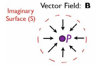
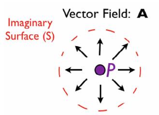
An example of positive divergence (Vector Field A) and negative divergence (Vector Field B). It can be seen that it is useful to imagine the black vectors as the motion of water at the various points around P to see if it is a source or a sink. iv

The mathematical definition of divergence is the sum of the rate of change of the vector function in each direction. This is expressed algebraically as:

Or in words: Divergence of A = (rate of change of A in x-direction) + (rate of change of A in y-direction) + (rate of change of A in z-direction)

Some examples of calculating divergence mathematically are as follow

Example 1.1

Consider a point P in a vector field E(x,y,z) with vectors around it as shown. To calculate the divergence at P, we calculate the rate of change in the x and y directions, as we can assume no change in the z–axis in this 2-dimensional diagram. iv

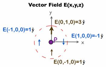
So the divergence at P is positive (+1), meaning there is more flow out of the point than into it, so it is considered a source (which can also be seen intuitively from the diagram)

Example 1.2

We can now mathematically calculate the divergence at any point in a vector field A(x,y,z) using some calculus.

This equation will now tell you the divergence at every location in space for the vector field. i.e. if we want to know the divergence at the point (x,y,z)=(3,2,1) then:

2.3. Curl

The third key mathematical concept which we need to understand Maxwell’s Theory of Electromagnetism is curl, which is displayed by the del operator followed by a cross. Whilst divergence is the measure of the flow of a vector field, curl is the measure of rotation of a vector field about a specific point. That is - if you were to drop a twig into the “fluid” and fix its centre, would it rotate at all?

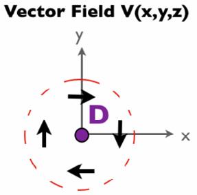
Whilst it is relatively intuitive to see whether divergence is positive or negative once you have its definition, curl is a little harder to determine. I will illustrate how positive and negative curl is chosen through a non-numerical example:

Example 2.1

We can see intuitively that there is a curl at point D just by imagining that the arrows represent a fluid flow as we did before for divergence. The rotation is clearly clockwise about D, but is that a positive or negative curl? Firstly, we need to determine the axis of rotation. As the curl is in the x-y plane, the axis of the curl is taken to be the z-axis. In addition to this, curl follows a right-hand rule, meaning if you point your right thumb in the direction of the positive axis about which the rotation is happening (the +ve z-axis in this case) then your fingers will wrap around the thumb in the direction of positive curl. For this example, the curl would be positive if it were anticlockwise, so the z component of the curl at D is therefore negative. v

The mathematical definition of the curl for a vector field A is defined as:

Or in words: Curl of A = (How much spin in the y-z plane) x + (How much spin in the x-z plane) y + (How much spin in the x-y plane) z A note is that as curl is the measure of rotation of a 3-dimensional vector field, we get a 3-dimensional result.

An example of calculating curl mathematically of vector field H is as follows:

Example 2.2

To calculate the curl we first need to work out all the partial derivates needed:

Or it could be written in the form

This vector function for curl can be evaluated for any point in space (x,y,z). Vx and V y will always be equal to the constant -1, but it can be seen that Vz depends on the value of x for the point.

2.4. Historical Context

It is also useful to understand the history leading up to Maxwell’s revolutionary work (published in 1873), with the most significant influence being the work of Michael Faraday, whose portrait was also hung on Einstein’s study wall.

Michael Faraday was born to a poor family and was not able to receive any sort of formal education. He managed to get a job as an assistant at the Royal Institution in London and was eventually allowed to conduct his own experiments. Through these experiments, Faraday found that moving a magnet inside a loop of wire would generate electricity in the wire, and the reverse: that a moving electric field generates a magnetic one. The relationship between electricity and magnetism was completely unknown at the time and these observations proved Faraday as one of the greatest experimentalists of all time.

Due to his lack of a formal education, Faraday did not have the mathematical fluency to describe these observations. He instead filled his notebooks with diagrams of lines of force which looked like the patterns iron filings made when surrounding a magnet, which are now what we know as field diagrams. However, what many people will not know is that the entire concept of a field, which is one of the most important ideas in all of physics was actually invented by Michael Faraday. The study of fields required a new branch of mathematics to complete calculations. It was called vector calculus and was created by the Cambridge - educated and mathematically gifted James Clerk Maxwell. It was Maxwell who was able to summarise the entirety of electricity and magnetism in four single equations, as he had the mathematical literacy that Faraday lacked. This was no easy feat, and the achievement is summed up perfectly in another quote from Einstein: “Any intelligent fool can make things bigger and more complex. It takes a touch of genius and a lot of courage to move in the opposite direction.”

3. Maxwell’s Equations of Electromagnetism

Whilst I explained divergence and curl mathematically as well as conceptually, I will focus more on the physical meaning of the four equations themselves, as it is much more important to understand what equations actually mean instead of just being able to plug numbers into them. After explaining the conceptual meaning of all four laws, I will dive into the implications and importance of them on a wider, more general level.

3.1. The First Equation: Gauss’ Law

This equation essentially dictates how the electric field behaves around electric charges. Gauss’ Law is: where: E is the electric field ρ is the electric charge density ε0 is the permittivity of free space (8.85 x 10-12 F.m-1)

The equation shown above is Gauss’ Law in point form, meaning for any point in space around a charge, the divergence of the electric field is directly proportional to the charge density at that point.

Gauss’ Law can also be used to derive the equation to calculate the magnitude of the electric field outside of a spherical charge (note that E is not in bold):

This is an inverse square law, mathematically similar to Newton’s Law of Gravitation. Like gravity, the electric field drops off away from the surface of a charged surface in proportion to the square of the distance. i.e. the electric field is four times weaker if you move twice as far away from it. A note is that the electric flux through a surface is the amount of electric field that pierces that surface.

Gauss’ Law can be written in integral form, where it states that the net electric flux (Φ) through a closed surface S is given by: where the integration is carried out over the entire surface S. Here, Gauss’ Law states that the total electric flux exiting any volume is equal to the total charge inside it. So if there is no charge within a volume, the net electric flux leaving it is zero. A positive charge inside will result in a positive amount of electric flux leaving, and a negative charge will result in a negative amount leaving (essentially meaning the electric flux will enter the volume).

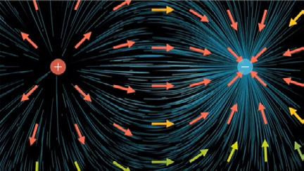
This form of Gauss’ Law explains that positively charged regions act like sources for the electric field, and negatively charged regions as sinks, as shown in the diagram on the left. A combination of the integral form of Gauss’ Law and the inverse square law explains the shape of the electric field around a positive charge next to a negative one, as shown. iii

3.2. The Second Equation: Gauss’ Law for Magnetism

The second of Gauss’ Laws is similar to the first one for electric fields, only here it states that the divergence of the magnetic field B at every point is equal to zero: or in integral form:

If we think of the magnetic field as a fluid flow once again, then this law essentially says that that fluid would be incompressible, acting just like water with no sources and no sinks. Another conclusion that can be drawn from this equation is that magnetic monopoles (meaning a north or south pole of a magnet by itself) can not exist, as they would cause a non-zero divergence of the magnetic field. If you chop a bar magnet in half, you always end up with north and south poles in both halves; there is no magnetic equivalent of a positive or negative charge by itself in an electric field.

Similarly to electric fields however, Gauss’ Law for Magnetism describes a very similar shape and strength for the magnetic field around a magnet: that being a closed loop from the north to the south pole as is observed when iron filings are placed around a bar magnet.

3.3. The Third Equation: Faraday’s Law of Induction

This is arguably the most famous of the four equations and is accredited to Michael Faraday as he was the first person to observe the experimental evidence of this law (as explained in section 2.4) Faraday’s Law is formally written as

In this form, it is relatively easy to see what the equation means: The rate of change of the magnetic field B (multiplied by the magnetic constant μ0) depends on the curl of the electric field E. Or even more simply, a changing electric field produces a magnetic field. Like all of Maxwell’s Equations, Faraday’s Law can also be written in integral form:

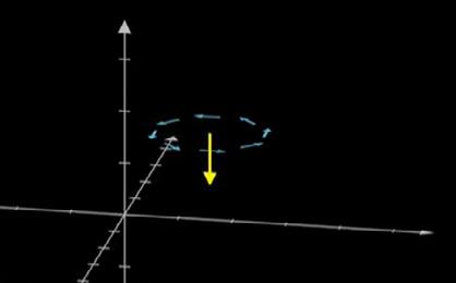
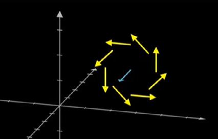
This can be demonstrated through a simple diagram. iii The blue vector field represents the electric field, which clearly has a curl. Using the method described in section 2.3, we can determine that the curl is positive and about the z-axis. Therefore, using Faraday’s Law of Induction, we can see that the rate of change of the magnetic field (which is the yellow vector here) will be in the negative direction of the z-axis, as shown.

Many of the experiments conducted by Faraday involved magnetic coils and circuits. Another way that Faraday’s Law can be written in the context of a magnetic coil is: Where ε is the total emf induced across a coil and ΦB is the magnetic flux within the coil.

So in words, this form of the equation states that the magnitude of the total emf induced across the coil is equal to the rate of change of magnetic flux in it, with the emf always induced in the opposite direction to the change in flux. The reason for the emf being in the opposite direction to the change in magnetic flux is due to the conservation of energy: if energy is lost in one form in this case, it will be converted into another form in the opposite direction.

3.4. The Fourth Equation: Ampere’s Law

Ampere was experimenting with forces on wires carrying electric current around the same time that Faraday was working on his similar research in the 1820s. Neither scientist had any idea that around 50 years later their work would be unified by Maxwell in simple, elegant mathematical laws. Ampere’s Law describes the opposite effect of Faraday’s Law, and is therefore mathematically similar:

Where: B is the magnetic field [T]

J is the electric current density [A/m2]

E is the electric field [Vm-1] μ0 is the magnetic permittivity of free space (magnetic constant)[1.26 x10-6 NA-2] ε0 is the electric permittivity of free space (electric constant)[8.85 x10-12 Fm-1]

Visually, this is the most complex of the four equations, combining curl, the magnetic and electric fields and electric current density as well as both the electric and magnetic constants. However, the physical meaning of the fourth and final of Maxwell’s equations is no more complex than Faraday’s Law.

4. Linking Concepts and Drawing Conclusions

If we neglect all the physical constants and J, this equation is essentially just the opposite of Faraday’s law. It states that the rate of change of the electric field depends on the curl of the magnetic field. Note that this time there is no negative before the partial derivative, which means that the direction of the electric field is the same as the direction of the curl of the magnetic field. For example, in this diagram on the left iii the curl of the yellow magnetic field is negative, and therefore so is the direction of the electric field.

4.1. Light

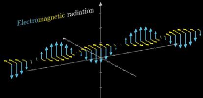
It has been shown both mathematically and conceptually that a changing magnetic field induces an electric field and vice versa. These effects had been observed experimentally, as explained in section 2.4 before Maxwell summarised them mathematically. However, his idea for the ages was: what if a changing electric field created a magnetic one that then in turn created another electric field etc? The conclusion that Maxwell drew from this was that the result of this back-and-forth motion would be a moving wave, with constantly alternating electric and magnetic fields turning into one another. Using vector calculus, Maxwell calculated the speed of this new “electromagnetic” wave to be 310,740,000 ms-1 which he was surprised to find was incredibly close to the speed of light (within experimental error). Maxwell was struck by this and wrote prophetically “We can scarcely avoid the inference that light consists of the transverse undulations of the same medium which is the cause of electric and magnetic phenomena”. 4.2. Radio

This diagram iii is a way of visualising the constant alternating oscillations of the electric and magnetic fields, which Maxwell realised was a new type of wave. As a result of the electric and magnetic fields always being perpendicular to one another, electromagnetic waves were classed as “transverse” waves.

As is often the case in physics, discovery was followed by invention. Maxwell had found this new type of wave and had proved that light was one of its many forms. However, the next challenge was to artificially produce these Maxwell waves in the laboratory, which was first done in 1886 by Heinrich Hertz. He achieved this with a simple setup by having an electric spark generator in one corner of his lab and a coil of wire several feet away from it. When Hertz would turn on the spark, he was able to generate an electric current in the coil, thus proving that this new wave had travelled wirelessly from one place to the other.

The direct consequence of this experiment was released to the public less than a decade later in 1894, and forever changed human communication: radio. Today it is easy to take for granted being able to send and receive messages wirelessly over incredibly long distances at the speed of light, however when you stop to think about this there is something almost magical about it. We use the internet every single day for just about everything: working, socialising, storing data, ordering food, entertaining ourselves and so much more. This would all be impossible if not for the discovery of electromagnetic waves, the invention of radio and most importantly Maxwell’s Theory of Electromagnetism.

4.3. The Whole Spectrum

Visible light and radio are of course only two forms of electromagnetic radiation, and it did not take long for scientists to realise it, with some forms such as infra-red having been observed long before Maxwell’s time but only being able to be explained after his theory. In the present day, we utilise the entire electromagnetic spectrum in countless scenarios, from the most subtle of applications to entire machines which save countless lives daily. I am not going to go through every type of electromagnetic radiation and give all the ways that they have been used over the years for humanity’s benefit, as I am sure anybody can come up with a hundred examples just by looking around.

However arguably the greatest and most significant application of Maxwell’s equations was for the crucial purpose of powering the planet. Whilst traditional energy stores such as oil, coal and gas needed to be shipped across vast distances by various modes of transport, electrical energy can be sent over the same distances almost instantly through a network of wires and accessed at the simple flick of a switch.

This led to the legendary battle between Thomas Edison’s DC (direct current) and Nikola Tesla’s AC (alternating current) which took place in the late 1880s and early 1890s. The difference between the two options was that DC always moves in the same direction and never varies in voltage, whereas in AC power the direction of the current reverses usually fifty or sixty times per second.

Whilst I will not delve into the legendary “War of the Currents” in too much detail (there is a very good film all about it which I recommend ) I think it is fair to say that the reason that AC eventually won was due to Tesla’s better grasp of Maxwell’s Equations. The key to the war was in reducing the energy losses that engineers knew would occur over the many miles of wires. Higher voltag- es meant lower currents and therefore less energy losses to heat in the wires, but the problem with Tesla’s higher voltage AC was that it was simply too dangerous to be introduced into homes, whereas Edison’s DC was much safer. The trick that Tesla used to solve this problem - and a genius application of Maxwell’s equations - was to use transformers. As AC electricity is constantly changing, it can be converted into a magnetic field which can then be converted back into another electric field, but at a lower voltage. DC current cannot be transformed in this way due to it having a constant voltage that does not alternate. (As you will recall, the third and fourth equations state that electromagnetic induction can only be done with a changing electric / magnetic field) So the solution that we still use today was to use efficient, high-voltage cables for the long distances between the power plants and cities, and then to transform the electricity into much safer, lower voltages when it enters homes.

4.4. Conclusion

By 1900, Maxwell’s Equations of Electromagnetism and their countless applications had brought about both a new fundamental understanding of nature as well as the huge economic prosperity that resulted from the birth of the electrical era. At the turn of the century, prominent scientists were proclaiming “the end of science” as it was thought that everything that could be discovered had been discovered. It seemed that the combination of Newton’s and Maxwell’s equations formed a “theory of everything”.

What physicists did not realise was that the work of these two giants of science was incompatible. However, one man would realise it soon enough and change the world. He was born the very same year that James Clerk Maxwell died (1879), and he would later hang the portrait of the great physicist on the wall of his study.

References

Merriam, A. (2020) The wall of Albert Einstein’s home bears the portraits of 3 scientists [online]. Last accessed: 27/07/2022. Available at: https://www.cantorsparadise.com/the-wall-of-albert-einsteins-home-bears-the-portrait-of-three-eminent-scientists-f84d0c458dce

Maxwells-Equations.com (2012) Vector Functions [online]. Last accessed: 27/07/2022. Available at: https://www.maxwells-equations.com/vector-functions.php

3Blue1Brown (2018) Divergence and Curl [online]. Last accessed: 27/07/2022. Available at: https://www.youtube.com/watch?v=rB83DpBJQsE&t=814s&ab_channel=3Blue1Brown Maxwells-Equations.com (2012) Divergence [online]. Last accessed: 27/07/2022. Available at: https://www.maxwells-equations.com/divergence.php

Maxwells-Equations.com (2012) The Curl [online]. Last accessed: 28/07/2022. Available at: https://www.maxwells-equations.com/curl/curl.php

Kaku, M. (2021), The God Equation, Great Britain, Allen Lane - Penguin Books Baker, J. (2007), 50 Ideas You Really Need to Know: Physics, London, Quercus Editions Ltd Halliday, D., Resnick, R., Walker, J. (2014), Fundamentals of Physics, 10th Edition, USA, Wiley Maxwells-Equations.com (2012) Gauss’ Law for Magnetism [online]. Last accessed: 29/07/2022. Available at: https://www.maxwells-equations.com/gauss/magnetism.php

UniversalDenker Physics (2019) The 4 Maxwell Equations [online]. Last accessed: 30/07/2022. Available at: https://www.youtube.com/watch?v=hJD8ywGrXks&ab_channel=Universaldenker%E2%9A%9BPhysics

The Current War (2017) [Netflix] Available at: https://www.netflix.com/gb/title/80192838?s=i&trkid=13747225&vlang=en&clip=81316498

Introduction: