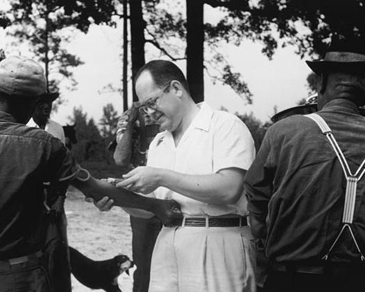
FIGURE 2.0 | WiFi location data used to investigate the spread of SARS-CoV-2 at a public university.
CHAPTER 2
Epidemiology
Selected Key Terms
Here are a few essential terms used in epidemiology. By the end of this chapter, you should be able to apply these terms and understand how they relate to other critical concepts.
Asymptomatic Transmission
Bias
Case
Case Fatality Rate
Case Investigation
Cluster
Contact Tracing
Epidemiology
Exposure
Hypothesis
Incidence
Index Case
Prevalence
Reproduction Number (R0)
Risk Ratio
Superspreader Event
Transmission Rate
Big Concepts
2.1: Introduction to Epidemiology
The principles of epidemiology have been practiced throughout human history to help us understand how the natural world impacts our health. Even before humans understood pathogens to be the cause of infectious diseases, scholars investigated their spread using careful observations and extensive data curation. Their contributions, from Hippocrates’ coining of the term ‘epidemic’ to Ibn Sina’s Canon of Medicine, and Graunt’s introduction of statistical inference, have helped shape the field of epidemiology today.
2.2: Epidemiology Concepts and Definitions
Epidemiology uses interdisciplinary collaboration and a shared understanding of key concepts to develop outbreak response strategies. Epidemiologists identify health-related phenomena, quantify observations, and review detailed records to draw conclusions. The ability to carry out this work requires shared definitions of many central ideas, such as what constitutes a “case” of a disease, an “exposure” that may have led to it, and a recognition of how an infectious pathogen might spread. These concepts make it possible to conduct investigations that reveal how a pathogen was transmitted through the population.
2.3: Epidemiology Calculations
Various analytical tools yield insight into how a disease spreads, and the impact of certain behaviors and response strategies. Epidemiologists employ many standardized concepts and calculations to analyze and understand disease transmission. Some of the most important and informative statistical measurements include prevalence, incidence, and reproductive number (R0). These values are used to represent the impact of disease in a given population – as well as to reflect its changes over time – and can help assess what types of intervention might be most effective in reducing spread and illness during an outbreak.
2.4: Data Collection and Study Design
Well-designed studies and thoughtful interpretation of their results are at the heart of epidemiological discoveries. Epidemiologists are able to conduct research studies by breaking down major questions into hypotheses that can be tested, and gathering and analyzing data while limiting bias. There are many different types of studies that epidemiologists may choose to conduct including observational and experimental studies. For all types of studies, consideration of ethics and equity is crucial. Given that the work of epidemiologists directly describes and impacts the actions and lives of the general public, epidemiologists must be thorough, intentional, and diligent in designing studies and communicating their findings, ensuring that their results are accessible to their target audience.
Vick’s Video Corner
Watch “ Vick’s Video Corner ” as an entry point for this chapter.
2
Epidemiology 2
As you move through the chapter, you will gain a better understanding of the importance of the field of epidemiology and the many disciplines that contribute to it; the different concepts, calculations, and methods employed to evaluate a pathogen’s emergence, impact, and spread; and the approaches used to perform epidemiological studies and enact public health strategies in response.
It’s the year 1854, and your neighborhood in Soho, London, has been overtaken by sickness, and with it, panic. Locals are incredibly ill — vomiting, with watery stool. Shops are deserted, and details of the illness are plastered over every newsstand, along with warnings to avoid breathing in the toxic ‘miasma’ vapors that are believed to be responsible for the illness. It seems like no one truly understands where this sudden spike in illnesses came from and why only half of the square is affected.
You decide to get to the bottom of this. You travel around the neighborhood for the next few days, asking the local shopkeepers if they know anyone who has been infected. It doesn’t take long before the shop owners fill your list with names, and you begin to investigate how these individuals’ paths may have crossed. You decide to sketch a ‘dot map’ of Golden Square, a classic tool used to identify affected households on maps and mark the locations of the infected households. A pattern emerges from within the data – clusters of infected households have amassed in certain parts of the neighborhood.
Through your comprehensive investigation, you recognize that there must be something within that area that is responsible for the outbreak — otherwise, the cases would have been more evenly spread across the sector. Could there be a popular tavern selling contaminated food? Is there an animal or insect species that is carrying the disease within the area? Are people engaging in certain activities that are increasing their risk? As you run through the possibilities in your head, you pass by the nearby communal water pump on Broad Street. The concentration of cases that you have noted around this region – along with your own suspicions on how the disease is spread – helps you formulate the hypothesis that the water from the pump on Broad street must be the source of contamination.
“[Epidemiology’s] methods may be scientific, but its objectives are often thoroughly human.”
—Alex Broadbent, British Philosopher of Epidemiology
The bustling activity around the pump raises your suspicions; and the more you investigate, the more it appears that all cases are tied to drinking from the Broad Street pump, but you need to test your hypothesis in order to be sure. Despite the lack of support from local leaders, you convince the neighborhood watch to help you remove the handle from the water pump, rendering it unusable for at least the next few days.
Since beginning your investigation, the number of new cases within Golden Square has already begun to decline naturally. After the pump is disabled, you continue to notice the cases decreasing, and within just a few more days, the outbreak has ceased. Perhaps even more impactfully, you’ve triggered a seismic shift in how the world of science approaches, documents, and investigates issues of public health for generations to come. Your detailed research methods and careful hypothesis testing inspired leagues of scientists to follow your lead, formalizing the study of public health and infectious disease in the western world.
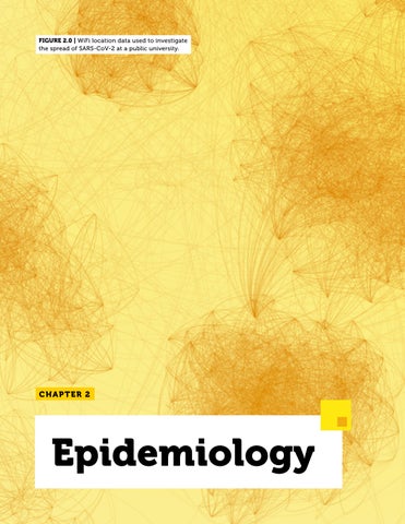
Congratulations! You are John Snow, known as one of the founders of modern epidemiology, and frequently credited with helping to control the mysterious 1854 London outbreak – which we now know to have been caused by cholera (Figure 2.1). Much of the literature presenting your contributions to the cholera outbreak in 1854 portray you as the first epidemiologist to use a map to visualize an outbreak. However, at least 60 years earlier in 1798, Valentine Seaman, an American physicist, mapped the yellow fever epidemic in New York City, and a number of other maps of infectious disease outbreaks predate the iconic Golden Square map. Whatever their origin, maps have been used to track epidemiological outbreaks for hundreds of years, and they are still a common practice today.
FIGURE 2.1 | Dr. John Snow and his famous ‘dot map’ of Golden Square. British physician and epidemiologist, remembered as one of the founders of modern epidemiology, and recognized for his contributions in solving the puzzle of the 1854 Cholera outbreak in London. This map, compiled in 1854 showed individuals affected by the disease during the outbreak in London, using lines to count deaths per household. It is unclear when exactly this map was made during the investigations of the outbreak, but it has become one of the most iconic disease maps in the history of epidemiology.
Scan this QR code or click on this link to view an interactive recreation of Snow’s map and explore how modern epidemiologists might have approached this same technique.
2.1: History and Introduction
Epidemiology is formally defined as the study of “incidence, distribution, and possible control of diseases and other factors relating to health.” Derived from the Greek epi, meaning ‘upon, among’, demos, meaning ‘people,’ and logos, meaning ‘study,’ the word “epidemiology” literally means “the study of what is upon the people.” Epidemiologists gather data about health behaviors and outcomes within the population, as well as key logistical information about timing, place, and even social contacts, to discover commonalities and differences between those who get sick and those who do not within a specific population. Their discoveries are frequently used to inform initiatives meant to reduce the burden of disease within the community.
It is important to appreciate that epidemiologists also study health outcomes that are not related to illness from infectious diseases, including heart attacks, car crashes, nutrition habits, and even the impact of treatments for disease. While these are all crucial health outcomes, for the purposes of this textbook, we will focus on epidemiology as it is practiced in the setting of infectious diseases. That said, we want you to know that many of the core principles you’ll learn about below are also useful to the study of many different health drivers.
Before diving deeper into the modern practice of epidemiology, let’s learn more about its history and a few of the milestones that have made the field what it is today.
Hippocrates, the ancient Greek physician you met in Chapter 1: Emerging Pathogens, who lived around 400 BC, was one of the first known figures to apply an analytical approach in his
pursuit of better understanding of health trends. Hippocrates cataloged the symptoms of many diseases within his four humors theory. In this theory health is governed by four humors, or liquids, that are found in the body and are each associated with a certain characteristic: black bile (melancholic), yellow bile (choleric), blood (sanguine), and phlegm (phlegmatic). This theory emphasized the idea that illnesses were caused by an imbalance of the “humors” in the body – a very different understanding than the previouslyheld belief that disease was caused at the will of supernatural forces. The theory continued to evolve with other Greek philosophers, such as Empedocles, who claimed that the humors were affected by the seasons and temperatures. He suggested that during the winter time, as the phlegm would increase with the cold weather, we would become more phlegmatic and develop more respiratory diseases. While now we know this is not exactly how it works, the humors theory remained an important framework to think about disease for hundreds of years.
Another of Hippocrates’s lasting contributions to modern science was his coining of terms, including epidemic, which he defined as a disease that occasionally “visits” a population (or is “upon” the “people”, as the Greek roots imply). He was the first to distinguish between epidemics, which occasionally arise within a population (like the 1347 bubonic plague), and endemics, such as modern chickenpox in the UK, which he described as diseases that are constantly present within a defined population. Endemic comes from the Greek word en, meaning ‘in, within’ and demos, meaning ‘people.’
As introduced in Chapter 1: Emerging Pathogens, the term epidemic is now defined as “the rapid
spread of an infectious disease throughout a given region” and is often interchangeable with outbreak, which indicates rapid spread but within a smaller geographical area. Both of these can be first seen as the appearance of a cluster, which is an unusual grouping of cases in time and space that may warrant further investigation. Later on, the term pandemic arose to define an epidemic with a scope across a large geographic area.
Another one of the many contributors to the developing field of epidemiology was Ibn Sina (also known by the Latin name Avicenna), who was a Persian and Muslim doctor, philosopher, and all around polymath (or person with a wide breadth of knowledge), born in the 10th century CE, in the kingdom of Samanid, the region now known as Uzbekistan. Ibn Sina became one of the most influential figures in medicine, compiling enormous amounts of information, including Greek, Indian, and Chinese medical practices, and publishing them in his Canon of Medicine; his text would become a standard text for health practitioners, and was still in use as late as 1650 –centuries after his death. Ibn Sina provided crucial insight into our understanding of the spread of both tuberculosis and water-borne diseases. He was among the first scholars to recognize that tuberculosis was passed from person to person, and was known for encouraging boiling water to eliminate impurities – a technique that is still used today.
In 1546, Italian physician Girolamo Fracastoro published his “germ theory” of disease as the first formal paper to predict that diseases were transmitted by small “seeds” which could travel between people and even contaminate objects. Although this idea may seem obvious now, germ theory was largely rejected at the time, in favor of a theory known as “spontaneous generation,” which posited that diseases and living organisms arose from non-living matter. During the time when
spontaneous generation was the leading theory, illnesses like tuberculosis and the black plague were the leading causes of death.
In 1668, using flies and meat, Francesco Redi performed an experiment that refuted spontaneous generation. Redi started by placing the meat in three different containers; one that was open to the air (where flies could get in), another that was covered with gauze (where flies would get near but not in), and a third that was tightly sealed (where flies could not get in or near). Maggots developed in the uncovered jars, but not in the gauze-covered nor in the tightly sealed jars. They did, however, also appear on the top of the gauze where flies could detect meat nearby and land. The experiment showed that maggots only appeared in areas that flies could access and lay eggs, proving that maggots are fly offspring, rather than the product of spontaneous generation (Figure 2.2).
Today, we now recognize that diseases like tuberculosis and the black plague are infectious diseases that are caused by pathogens that spread through physical routes, as germ theory suggests.
1668 experiment showed that maggots formed when flies could land and lay eggs in or near the meat and that the maggots were the offspring of flies, not the product of spontaneous generation.
Flask open Flask sealed Flask covered with gauze
FIGURE 2.2 | Experiment that refuted the spontaneous generation theory. Francesco Redi’s
Depending on the pathogen, these routes may include transmission through the air, insect bites, or contact with contaminated surfaces, bodily fluids, or blood products, among others. Over time, this more accurate understanding of germs and their spread allowed for the development of proper preventative measures, such as hand-washing, social distancing, bed nets, and vaccinations, which drastically reduced the burden of infectious diseases on the global population. This example of a development in our understanding improving outcomes demonstrates how the acquisition of new insight, and openness to change, are key to progress in most fields, especially public health.
The field of epidemiology took another leap forward in the 17th century when John Graunt began analyzing disease using statistical inference: the study of data to make predictions about a phenomenon of interest. Graunt combed through London’s death records to find patterns related to causes of death and features such as gender, season, and geographical setting. In one of his studies, Graunt noted that bubonic plague caused tens of thousands of deaths in 1625, but not nearly as many in each of the following years. He also found that the number of deaths caused by other infectious diseases tended to remain more constant over the same period of time. This finding confirmed bubonic plague’s status as an epidemic, as opposed to an endemic disease.
Graunt’s approaches enabled the development of clear research methodologies, ushering in the use of predictive models to better understand and improve health. More specifically, Graunt’s approach would become the cornerstone of what is now known as public health surveillance, which involves the collection and analysis of population-level health data, which is data that relate to the overall health of the population, rather than any specific individual. Many modern-day epidemiologists follow this tradition by using existing data and disease testing programs to monitor trends in populations, which is very helpful in monitoring norms around health behaviors. Examples of questions answered by surveillance epidemiologists might include:
1. Are young people smoking more or less than older people?
2. Are women more likely than men to suffer a stroke?
3. Are school absences due to respiratory illnesses becoming more common among elementary students?
Modern-day epidemiologists continue to utilize Graunt’s scientific and statistical foundations to analyze disease spread and allow public health professionals to devise appropriate interventions.
Stop to Think
1. Why are John Snow’s discoveries during the cholera outbreak in 1954 (Broad street water pump) considered groundbreaking for the time and the future of epidemiology?
2. What is the difference between germ theory and spontaneous generation?
3. How did the discovery and acceptance of germ theory help improve public health?
4. What are some modern-day applications of the historical advances described in this section?
2.2: Epidemiology Concepts and Definitions
Infectious disease epidemiologists today often start their work with the same basic approach as John Snow: by observing health trends within a group and asking themselves how and why those trends are occurring. Some questions might have relatively simple and well-known answers. For instance, why are individuals who live near a contaminated water source developing gastrointestinal infections? The answer is probably that pathogens are spreading through untreated water. However, other questions might have complicated answers. For instance, why are many patients exhibiting similar symptoms but testing negative for common pathogens? This question arose at the start of the COVID-19 pandemic, and lacked a simple answer. Although the scope and complexity of observations and questions change, the basic process remains the same, and this iterative process helps us to better understand our core problem.
By using population-level data ranging from community to state or national levels, epidemiologists can understand different aspects of a disease - where it is, who it’s affecting, and how quickly it’s spreading – to better understand how to control its spread. Sometimes, the key to untangling seemingly complex relationships is hidden in plain sight; think of the communal water pump in Golden Square, or how spoiled food in the cafeteria may be the source of the awful stomach illness everyone in your class is catching. Other times, the answer is more complex and epidemiologists must adopt a bird’s-eye view to assess multiple factors and understand how they interact. These situations require a multidisciplinary investigation - that is, an investigation undertaken by experts in multiple fields collaborating together. These
collaborations frequently include environmental scientists, economists, and social workers, as well as community leaders to help ensure that the study is undertaken in a culturally-appropriate manner. By investigating epidemiological phenomena and generating diverse data sets, epidemiologists aim to create robust, inclusive, and applicable studies that model populationlevel behaviors, and even trace the contacts of individuals that are infected.
How does all of this come together, and what does epidemiology really look like in action? Are epidemiologists a bunch of quirky scientists going around with magnifying glasses hunting for “disease data” in New York City subways, scolding people who touch the poles after coughing on their hands? Not quite. In practice, epidemiology is a collaborative and highly rigorous discipline, requiring clear hypotheses, precise terms and definitions, and powerful statistical tools to draw conclusions. These conclusions can then help epidemiologists identify whether those New York City subway poles are the real culprits of disease transmission, or if something else is at work.
Let’s now go over some of the most important basic concepts and key ideas in epidemiology, so that you can start your journey towards becoming a disease detective.
What is a ‘Case’?
Before collecting and reviewing data, it’s often helpful for epidemiologists to create a solid description of exactly what they are looking at, so an outbreak investigation will typically start with the description of a case. A case is defined as an instance of a particular disease or outcome of interest, i.e., getting in a car accident or being injured at work. In the setting of infectious
disease, this would be an individual presenting symptoms typical of an illness and confirmation of the illness with a diagnostic test.
Further, when studying a case such as health outcomes related to an infection, the epidemiologist must have a clearly defined and reliable way to determine if each recorded individual truly has a case of the disease of interest. This process is known as case definition; in other words, all the factors that must be present in order to consider any given observation as a “case.” Case definitions allow public health responders, in different places and at different times,to identify, treat, and perform work under a standard understanding of the disease. These definitions help to minimize the number of incorrectly-identified cases and ensure that true cases do not slip through the cracks. Many countries’ health departments establish national case definitions for diseases of concern. In the US, for example, the CDC provides the standard case definitions which are used by local, state, and territorial epidemiologists, along with other interested parties, and updates these definitions when necessary, for example, during an outbreak.
Early on, during outbreaks of novel pathogens, case definitions may be fluid and change rapidly as the understanding of the disease evolves. Over time, it will become more specific as additional information on the new disease accumulates. This evolution can quickly impact new research and policy recommendations. Sometimes researchers must even start responding to an outbreak before they even know what they’re looking for. For example, in the early stages of the US HIV epidemic in the 1980s, healthcare professionals noticed a trend of uncommon lung infections and the development of rare cancers. Researchers eventually identified the underlying
driver of these illnesses as HIV, which was destroying infected patients’ immune systems and leaving them vulnerable to lung infections.
For infectious diseases, we ultimately prefer the case definition to include detecting the pathogen itself in a clinical sample taken from an individual, a type of positive diagnostic test. We will learn more about diagnostic tests in Chapter 7: Diagnostic Tests. However, in times or places where testing is not available or adequate, or when it is not sufficient to determine a disease state of interest, we need to rely on other information. When there is potential uncertainty around the diagnosis, case definitions can be further categorized by the degree of certainty, marking a specific case as “suspected,” “probable,” or “confirmed.” The case definition may rely on a specific group of symptoms, such as the recognizable shallow white-ish red ulcers that appear in the mouth of a person infected with measles, paired with the disease’s less specific signs and symptoms like a fever and cough. For example, a positive SARS-CoV-2 result on a COVID-19 test is now generally considered as a case. However, where diagnostics are not available, fever and cough with new-onset loss of taste or smell might also be considered a COVID-19 case.
Exposure
A case tends to result from an interaction with one or many exposures. In the realm of epidemiology, exposure typically means any factor a person could have encountered that relates to – or might have contributed to – their specific health outcome. Typically when studying outbreaks and epidemics, we describe an exposure as a situation in which a susceptible individual comes in potential contact
with the causal pathogen. For example, in a 2020 outbreak of salmonella – a foodborne pathogen – that infected over 1,000 individuals across 48 states, researchers determined that a specific brand of red onions was linked to each case of salmonella. These results meant that consumption of that onion brand was a potential exposure, triggering a recall of the produce and ultimately ending the outbreak.
While contact with a pathogen is the key exposure for an infectious disease, there are other types of exposures that can have an impact. For instance, an exposure could be environmental, linking factors such as a region with high air pollution with an increased community risk to develop respiratory infections; or genetic, where people with the genetic disease sickle cell anemia are more susceptible to infection by salmonella and other pathogens that are less common in people without sickle cell anemia.
Case Investigation
Once epidemiologists have defined a case and identified potential exposures, they employ tools to identify instances of the disease in a population and develop a better understanding of its presentation at the community level. This task is called a case investigation. Today, modern epidemiologists use many of the same underlying concepts developed by the early epidemiologists to investigate cases, although the methods, tools, and technologies have been refined over the years.
In performing case investigations, epidemiologists try to answer five essential questions, known as the Five W’s of Epidemiology. These questions are typically asked at the individual level, and the data is then
compiled from the full population to develop a higher-level understanding of how the disease has moved through a population:
1. Who: who was infected?
2. What: what were the symptoms, course of illness, and ultimate diagnosis?
3. When: when did the person fall ill?
4. Where: where was the person before, during, and after their illness?
5. Why: why did this person fall ill? (e.g., risk factors, activities, potential causes, exposure to other infected people, etc.)
Two techniques, known as contact tracing and geolocation, can aid in answering the Five W’s, making them useful tools for case investigations. These techniques share many of the same principles as Snow’s dot map of cholera-stricken households, but with modern updates to data collection and visualization.
Contact tracing is the practice of (retroactively) documenting the movement of an infected individual through a population, noting key details like the people with whom they have interacted and the places they have visited. This method is used to help public health professionals and researchers better understand an outbreak’s spread, scale, and scope, help identify other cases, and find a way to contain it. For example, contact tracing was instrumental in Hong Kong during the 2002-2004 SARS outbreak, where epidemiologists were able to identify particularly high transmission between individuals living in the same households, and within healthcare facilities.
Contract tracing has two possible processes. The first starts with the identification of a case and
then moves forward in time; it’s a preventative initiative that aims to identify the individuals who have interacted with the infected person and therefore should be tested for the disease, and even isolated, to protect others who might be at risk for being infected. The second starts with a case and then works backward, trying to figure out who or what exposed this case to the disease. This process is known as source investigation, as it helps researchers retrace the illness to the initial source of the disease, and aims to find the initial source of introduction into the group of cases being investigated. Examples of source investigation findings might be the discovery that you became ill from sitting next to your coughing classmate, or that a local burrito bar is the cause of the food poisoning cases cropping up around the city.
Traditional contact tracing is an extensive analog process in which public health professionals interview, via phone or in-person, infected people. These interviews mainly focus around recent activities before and after the individual’s potential exposure to the pathogen. For example, the interviewers may ask “who have you visited or spent time with recently?” to determine their close contacts (who are likely to have been exposed). The investigation team may then also interview the identified contacts to determine whether or not they are ill and who else may have been exposed. Contact tracing may also be done passively through surveys that ask whether the respondent has recently come into contact with an ill person, and if so, whom.
Smartphones and Bluetooth technology have given rise to proximity sensing technologies, which can automatically catalog interactions between individuals by using their geographic location information. Using this technology for contact tracing and containment efforts can result in even more accurate results than pure recall alone.
Table 2.1: Basic Definitions in Infectious Disease Epidemiology
Term Description
Case
Exposure
Case Definition
An individual who has contracted the disease of interest.
The activity, material, or individual through which a susceptible person potentially came in contact with the causal pathogen.
The compilation of factors that must be present in order to consider any person’s presentation a “case”, frequently including a diagnostic result.
Case Investigation
The epidemiological process of working to determine key information about the disease of interest, frequently targeted toward answering the Five W’s of Epidemiology (Who, What, Where, When, and Why).
Similarly, geolocation techniques, such as the maps John Snow used, allow epidemiologists to track the places where infected individuals have visited pre- and post-illness. This can highlight potential sites of exposure and transmission as well as allow epidemiologists to observe a particular distribution of cases. Modern geographic information science (GIS) systems and software have the potential to greatly advance geolocation efforts. Many nations employ GIS technology to respond to infectious disease outbreaks on a broad scale, such as Israel’s national GIS database, which was developed in 1992 to control the spread of malaria within the country.
Since 2020, different contact tracing apps specifically focused on COVID-19 have been developed. COVID-19 contact tracing apps use Bluetooth and geolocation, and have been used in multiple countries, including Spain, Switzerland, and the UK. In the UK, this approach had a particularly large epidemiological impact. Released in England and Wales in September 2020, the UK National Health Service (NHS)
FIGURE 2.3 | Index case. This graphic shows an example of the progression of viral from the reservoir host, to the index case (who may or may not be the primary case), to more individuals, with the potential for epidemic proportions.
COVID-19 app has been used by 16.5 million people out of a population of 34.3 million smartphone users. App users were notified whenever they had been in close contact with another user reported as positive, as well as if they had been exposed by visiting a high risk location. They would also receive information about how to prevent further spreading and suggestions to quarantine after a close contact exposure notification. Although this is a rather new technology, this app proved to be a helpful community measure, and these strategies are being replicated to prepare for future threats.
These digital methods have demonstrated benefit, but as you can imagine, adverse feelings towards the technology may limit uptake. Concerns about digital privacy and government involvement in social contact tracing technologies can not only make the general public wary, but also make the technology dangerous to particular communities – notably undocumented people and survivors
of domestic violence. For these reasons and many more, these technologies need to be used thoughtfully and designed to protect the data privacy of users.
Index Case
By following the course of an outbreak back to its source, epidemiologists are often able to get a better understanding of who may have been exposed, how a disease may be spreading, or what risk the disease may pose to the population. The first case identified by health officials in an outbreak is referred to as the index case (colloquially known as “patient zero”); for known infectious diseases that are not endemic, this is often the first signal to researchers that an outbreak could be on the horizon (Figure 2.3). While the index case is the first identified case, it may not be the first individual to bring a pathogen into a specific population, who is known as the primary case. It often takes some
time before public health becomes aware of an emerging outbreak. As such, the primary case is very difficult to determine and often goes unidentified. For example, although extensive investigations unearthed potential primary cases of COVID-19, with current evidence pointing toward a singular transmission into the human population at a market in Wuhan, China, there is still ongoing debate about how this disease entered the human population.
As with all public health efforts, it is important that epidemiologists thoughtfully engage the individuals who represent these key, early cases with respect, dignity, and as much confidentiality as can be preserved while still tracing potential contacts effectively. We do not identify these early cases to place blame or shame on any particular person or health behaviors, but rather to better understand the characteristics of a pathogen’s spread through a given population and identify those who might be at high risk of infection and illness. Not only is a compassionate, non-judgemental approach the right way to treat others, but it may also help others with potential exposures to feel more comfortable in coming forward or receiving diagnostic testing.
Transmission and Transmissibility
As you learned in Chapter 1: Emerging Pathogens, transmission refers to the modes in which disease spreads: direct or indirect contact. Transmissibility is a related concept that reflects the degree to which a pathogen is able to spread from host to host. It is estimated with the reproduction number or R0, which we will study in more detail in the next section of this chapter. More specifically, transmissibility describes how easily a pathogen spreads, taking into account how
contagious the pathogen is, how susceptible the host is, environmental factors, and many other elements.
Environmental factors that can affect the characteristics of the pathogen, and therefore determine its survival and transmission, include temperature, humidity, pH,surface material, and many others which may vary from outbreak to outbreak (Figure 2.4). Host factors such as immunocompromised status, age, or anatomy of a target organ in a host’s body, can make the exposed subject more or less susceptible to transmission.
Yet another key measure we care about is the transmission rate — which is influenced by not only the biology of the pathogen or its host, but also various outbreak mitigation strategies or social drivers of disease like mask-wearing, vaccination, or access to a healthcare facility.
Transmission rates can be highly variable and often change in time, even in the context of one pathogen. For example, some people might fall ill and then not pass the disease on to anybody else. Some might become sick
FIGURE 2.4 | Environmental factors affecting pathogen transmissibility. A number of environmental factors, not just the pathogen’s inherent characteristics, affect how transmissible a pathogen is.
and pass the disease to close contacts like their family members or friends. Others, due to biology or behavior, might go on to infect many people. These individuals are known as superspreaders. For example, a superspreader could be a person who delivers groceries and comes in contact with many individuals, or a music tour manager that attends multiple large concerts per week. They can also be someone who was part of a superspreader event, which are often large events, where one or just a few primary cases pass the disease on to many people. You will learn more about superspreaders and superspreader events, and their effect on the epidemiological analysis of transmission, in section 2.3: Epidemiology Calculations. For now it is just important to appreciate that transmission rate can be highly variable – even across seemingly similar situations – and it is important to understand its many facets in order to identify appropriate interventions.
Another notable type of transmission is asymptomatic transmission , a mode made well-known by COVID-19. Asymptomatic transmission occurs when an infected
individual presents few to no symptoms of the disease, but is still contagious, and passes the pathogen along to at least one other person. We will learn in more depth what a symptom is and how health providers use these to diagnose a disease in Chapter 3: Clinical Symptomatology. For now, keep in mind that symptoms are clues we can use to detect that something is not right in someone’s body, and that they therefore may be ill. The absence of symptoms in asymptomatic individuals makes it harder for patients and epidemiologists to recognize that they are ill, and realize the danger that they pose to their communities. Furthermore, asymptomatic cases can be hard to document and quantify, as asymptomatic individuals are less likely to seek out testing and/or care and frequently go unnoticed. This means the percent of cases that are asymptomatic is often unknown, or greatly underestimated. Amid COVID-19, epidemiologists have been especially mindful of this stealthy reality, and continue to recommend cautious social guidelines in an outbreak setting, even for individuals who aren’t visibly sick.
Stop to Think
1. List the 5 W’s of Epidemiology and a contextual question for each (e.g., Who: who was infected?)
2. Create an example of a Case, Case Investigation and Exposure.
3. What are the particular threats posed by asymptomatic transmission?
2.3: Epidemiology Calculations
Now that you understand the basic concepts of disease transmission through a population, let’s learn how epidemiologists track, assess, and interpret this movement. We’ll start by introducing the statistical concepts that epidemiologists use to quantify spread.
Prevalence
The prevalence tells us how many cases there are of a certain disease in a population at a particular time. You can think of prevalence like a snapshot that tells epidemiologists what diseases exist in a particular setting or community. To calculate it, we divide the number of cases at a given time by the total number of people in the population of interest at the same time.
Table 2.2 Hypothetical point prevalence example key values
Date: June 15, 2021
Location: San Miguel Chapultepec, Mexico City
Population: 3000
Cases of Chickenpox: 6
Prevalence=
# of existing cases at the given time
x 100
Population size at the given time
There are two types of prevalence: point prevalence and period prevalence. Point prevalence is the number of current cases at an exact point in time. Period prevalence is the number of cases of the disease at a longer interval of time – such as a year.
Let’s work through a hypothetical example, starting with point prevalence. Let’s say that on June 15th, 2021, 6 individuals within the San Miguel Chapultepec neighborhood of Mexico City had an active case of chickenpox. If the total population of the neighborhood was 3000 people, the prevalence within that population would be 6/3000, or 0.2%. It’s important to recognize that the prevalence only reflects active chickenpox cases - the total number
Prevalence: 6/3000 = 0.002 x 100 = 0.2%
3000 6
Note: The numbers provided on this table were not taken from a reported outbreak. We made them up for simplicity of the example. If you would like to learn more about a real scenario where the incidence of a disease was calculated in an epidemiological study, we recommend you take a look at the article linked below: “Transmission from vaccinated individuals in a large SARS-CoV-2 Delta variant outbreak.”
Scan this QR code or click on this link to check out a scientific publication about a SARS-CoV-2 Delta variant outbreak in 2021.
of people who have had chickenpox and recovered are not reflected in the numerator. While the prevalence gives us insight into a particular snapshot of time, in this case June 15th, it cannot tell us how quickly a disease may be moving through a population. Finally, it is important to recognize that the prevalence we report only includes cases of which we are aware. Thus, the true prevalence of a disease in the community is frequently higher than we recognize.
In our hypothetical scenario, period prevalence would be calculated in a similar manner. Let’s say, for instance, 150 individuals within the San Miguel Chapultepec neighborhood of Mexico City had a case of chickenpox in the year 2021. Assuming the same total population of the neighborhood of 3000 people, the period prevalence within that population would be 150/3000, or 5%, during 2021.
US weekly COVID-19 cases between January 29th, 2020, and December 14th, 2022
FIGURE 2.5 | US Weekly COVID-19 cases reported to CDC. This graph shows the weekly cases of COVID-19 between January 29th, 2020, and December 14th, 2022. The prevalence over time allowed for identification of different “waves” of infection (where the curve grows due to an increased number of cases) and helped us think about “flattening the curve” (where the curve shrinks due to a decreased number of cases). COVID-19 data tracked by the CDC can be found in this site in which you can play around with different variables to observe prevalence of the disease in the US population.
The average duration of a disease affects its prevalence (both point and period). The shorter the duration of a disease, the fewer people will have it at any point in time, and thus, the lower the prevalence. Conversely, a longer-lasting disease will drive the prevalence up, because the longer a disease lasts, the more likely it is that an infected individual will still be ill when prevalence is recorded. . It’s also important to appreciate that prevalence is affected by how deadly the disease is, as well as how quickly people recover. Both quick recovery and high mortality drive down the prevalence at any time by removing cases from the numerator.
While it does not give any information about the time outside of the observation window –past or future – prevalence provides us with key details about the number of cases within a
Scan this QR code or click on this link to view a weekly US COVID-19 case tracker broken down by state.
population at a specific time. For starters, it can give us a “baseline” for the specific health event we’re concerned with, letting us know how many cases we would typically expect to find in the population under normal conditions. This is crucial information; by determining the usual, expected number of cases, we can recognize whether or not our current number of cases is unusually high and qualifies as an epidemic. More broadly, capturing case counts at different points in time allows epidemiologists to track variation in prevalence over time and place, to see not only when outbreaks start, but when they spike or subside (Figure 2.5).
Observing a spike may indicate that new response initiatives need to be put in place in order to “flatten the curve”, which describes the aim of trying to avoid a steep peak in prevalence so that hospitals and other resources are not overwhelmed by the outbreak (Figure 2.6). At the height of the COVID-19 pandemic, initiatives aimed at flattening the curve included wearing masks, social distancing, and setting specific isolation guidelines. While these didn’t stop all instances of transmission, they at least reduced the number of cases that appeared in a short window, which greatly helped keep the healthcare system from collapsing altogether.
Outside of an outbreak setting, by establishing the scale of a problem, prevalence can help epidemiologists set public health priorities and inform resource allocation. For example,
prevalence can be used to compare the relative burden of disease between groups; inter-community variation in the prevalence of a specific disease is likely reflective of (lack of) access to various resources like testing, treatment, and vaccines. For instance, we could calculate the prevalence of chickenpox in multiple neighborhoods within Mexico City and assess their respective disease burdens at that specific point of time. All things being equal, we would expect the prevalence to remain fairly consistent across the neighborhoods. However, if we were to observe a large difference in the prevalence, it may indicate underlying inequities or disparities, and this might prompt efforts to better support the communities where chickenpox was disproportionately prevalent or possibly underreported due to lack of resources.
2.6 | “Flattening the curve.” Tall peaks in cases can overwhelm hospitals and other healthcare resources, causing worse outcomes for all – even those who do not have the disease. Instituting protective measures can help reduce the prevalence of a disease to a level that is manageable, even if the spread is not fully stopped yet. On this graph, we show how the prevalence curves can look when no protective measures are taken versus when protective measures are taken, as well as how initiatives to “flatten” the curve depend on the healthcare system capacity.
FIGURE
Incidence
When public health experts aim to assess the risk of acquiring a disease, they turn to the disease’s incidence, which is the number of new cases within a population over a given period of time. It is important that we only include the population’s susceptible people in the calculation as new cases cannot arise in people who are not susceptible to the disease. Including non-susceptible people in the study would artificially deflate the calculated risk. For example, if we were calculating the risk of uterine cancer, including people who do not have a uterus in the denominator would make uterine cancer seem like half of the risk that it is.
There are a few different ways to calculate incidence, with some being more complicated than others. We’ll describe a relatively simple one here, known as incidence proportion or rate, as an example. The incidence proportion helps us understand how many individuals who are at risk of developing the disease actually became infected during the time interval of interest.
Incidence
Proportion
# of new cases during the given time interval # of susceptible people at the beginning of the time interval
Given that incidence describes change over time, it is crucial to not only define but also communicate the given time period when discussing incidence. For example, incidence could be described over one month, one year, 10 years, or any other selected period of time. It is also crucial to realize that incidence is not affected by death or recovery, as it is not affected by the duration of the cases, just the fact that they arise.
Let’s take the chickenpox example again, and say that only 1000 people in the Condesa neighborhood of Mexico City have had neither chicken pox nor the vaccine; this means only 1000 people of the total population in that neighborhood were still susceptible to chickenpox (since both the vaccine and previous infection would have granted immunity). In 2021, 150 of those people became infected with chickenpox. This would give an incidence proportion of 150/1000 = 0.15 cases per susceptible person over the course of 2021.
Prevalence and Incidence Together
Data regarding prevalence and incidence can be very powerful when taken together, as they help to capture a dynamic situation. The relationship between prevalence and incidence, as well as how they’re affected by recovery and death from the disease can be visualized using the metaphor of a bathtub (Figure 2.7).
FIGURE 2.7 | Prevalence and incidence describe different phenomena that contribute to the same system. They can be thought of as the system in this image, with the waterline of the tub representing the prevalence, and the rate of entry of the water as the incidence. Both recovery (evaporation) and death (leak) affect the prevalence, but they do not affect the incidence.
Incidence can be thought of as the tap, introducing new water to the tub; the water acan be flowing in at many different rates. Prevalence is represented by the water line of the tub, i.e. how much water it contains.
There are two ways that water can leave the tub: evaporation and a leak. In this example, evaporation reflects recovery, while a leak represents mortality from the disease. Notably, both evaporation and a leak only affect the waterline, not the flow of the tap. Similarly, recovery and death only affect prevalence, not incidence.
Risk Difference
Risk difference — also known as attributable risk or excess risk — is the difference between the incidences of disease in a group exposed to a certain risk compared to an unexposed group; importantly outside of the exposure, the groups should otherwise have similar characteristics. You can calculate the risk difference by subtracting the unexposed group’s incidence from the incidence of the exposed group.
observation, multiplied by the number of years that they are observed. Meanwhile we’ll say that female non-smokers were found to have a stroke incidence of 18 per 100,000 person-years. Since the two populations are otherwise similar, it would be reasonable to attribute this excess risk to their smoking exposure. We can therefore calculate that the risk difference is 32 per 100,000 people–years (50-18); for those curious, the risk difference using real-world data is 31.9. This means that female smokers are at much higher risk of having a stroke than their nonsmoking counterparts, and that successful anti-smoking campaigns could eliminate almost 32 strokes per 100,000 person-years.
Risk Ratio
Another measure commonly used to examine the risk posed by a particular exposure is a risk ratio, which is also a measure to compare the risk for two groups. The general formula is as follows:
This gives a statistical estimate for how many of the observed outcomes can be attributed to the exposure of interest. For example, let’s use numbers that have been mildly modified (just to make the math easier) and say that during a one-year-long study of 100,000 female smokers, 50 of them experienced a stroke. The incidence is then defined as 50 per 100,000 person-years. A personyear is the total number of people under
A risk ratio greater than 1 tells us that the given exposure likely increases the risk of a given outcome, whereas a risk ratio less than 1 indicates a protective factor, which is a factor that decreases the risk of the outcome. An example of a protective factor might be the fact that exercise protects against heart disease. A risk ratio close to 1 tells us that the exposure likely does not significantly affect the outcome either way.
Let’s set up the risk ratio using the information we have from the female smokers and stroke example above:
The resulting risk ratio 2.78 tells us that smoking nearly triples the risk of stroke in women.
Table 2.3
Comparing Risk of Strokes in Female Smokers and Non-smokers
Location: US Population:
- 18/100,000 = 32/100,000 or 32 per 100,000 people-years
Ratio: (50/100,000) / (18/100,000) = 2.78
In the context of infectious disease, risk ratios can be utilized to assess a particular population’s relationship to an exposure and outcomes in the following way; let’s say that there is a norovirus (which is a stomach bug) outbreak at a very small local school, and 50
Table 2.3 Risk Ratio of Salad Consumption on
Illness
out of the 100 students get sick. All of the students are interviewed about what they’ve eaten in the last 48 hours; if 40 out of the 50 ill students say that they had a salad, and only 5 of the 50 unaffected students report having salad, the resulting risk ratio of would make us very suspicious of the salad, or its components (perhaps the lettuce).
Case Fatality Rate
Another important epidemiological question is how often a given disease results in death, since it is a strong indicator of a disease’s severity and our required level of concern. This can be calculated in the case fatality rate (CFR), also referred to as case fatality risk or case fatality ratio. CFR is the proportion of individuals with a disease in a population who die from that disease during a specified time period. Relatively easy to interpret, this proportion can show you just how deadly a disease can be within a population. Its increase or decrease in response to different public health initiatives can highlight just how effective the interventions are at prolonging life and improving well-being.
To calculate CFR, you divide the number of individuals who have died from the disease by the total number of individuals in the population with the disease in a specified time period. CFR’s accuracy depends on all cases actually being identified. If the number of individuals who have the disease is underreported, which is often the case, the estimated CFR will seem higher than the true death rate from infection with the pathogen.
The CFR differs from mortality rate, which is calculated by dividing the number of deaths from the disease by the total susceptible population. The mortality rate represents the entire susceptible population’s risk of dying from the disease, not just those infected with the pathogen. The mortality rate is thus affected by the overall prevalence of the disease in the population. Even if the CFR for a disease is high, a low prevalence may cause the overall mortality rate to remain low.
# of deaths among cases due to disease
Mortality Rate
Total population susceptible to disease
Excess Mortality
When an individual suffers from a disease, they have a higher risk of dying from not only that disease but also other factors and complications. These factors and complications are potentially unrelated to, but exacerbated by, the disease itself. In the context of infectious disease, as time goes on, it can be increasingly difficult to determine if an individual suffering from a disease died as a direct result of the infection, or from a secondary, or underlying factor.
Similarly, outbreaks might have broader societal impacts that may increase the number of deaths; they may force hospitals to be overwhelmed or to close their “nonessential” services, including cancer screenings, well-child check-ups, and a number of other preventative services, which can have potentially fatal effects down the line. Outbreaks may also dissuade people from seeking care. For example, if there is an Ebola outbreak, people with severe malaria symptoms might be less willing to present to
the hospital to receive critical care, for fear of catching the more fatal Ebola virus while there. Additionally, if people are required to follow stay-at-home orders during a pandemic, they might try to self-medicate using alcohol and other drugs, running the risk of a fatal overdose. All of these factors can contribute to the increase in mortality during an outbreak.
To contextualize the impact of an outbreak, epidemiologists review population-level information and often look to calculate excess mortality (EM). Excess mortality is the difference between the observed number of total deaths in a population at a specified time period and the number of deaths one would expect in a ‘normal’ time period, often obtained from real-life data of the same population during non-crisis times.
Excess Mortality -
= # of deaths in population during this time period # of deaths in population in a ‘normal’ time period
Excess mortality is meant to capture the entire fatality burden of a disease, rather than just the deaths directly caused by the disease itself. For example, if a small town suffered 2,000 deaths during August 2020, the first year of the COVID-19 pandemic, but just 1,600 deaths the August before in 2019, they would have endured 400 excess deaths. Some of these deaths might be due to COVID infections, but some might be due to other factors, such as inadequate resources at a hospital strained by the ongoing pandemic. While there will of course be variation from year to year given random factors, an increase in mortality that is far greater than the variation seen between previous years would indicate the excess burden of COVID-19.
Reproduction Number (R)
One of the most well-known tools in an epidemiologist’s arsenal is the reproduction number (R0) (pronounced R-naught). The reproduction number describes the transmission rate of a disease and has different variations depending on the population being studied. R0 is known as the basic reproduction number, which refers to the average number of secondary casesnew cases of a disease caused by a single infected person within a population that is fully susceptible to the disease (Figure 2.8).
R0 depends on the assumption that the entire population — or at least an overwhelming portion of it — is susceptible to the disease. However, this assumption is not always the case, given that immunity to various diseases can be fairly common. For example, much of the contemporary US population is vaccinated for chickenpox at a young age; thus, R0 would not be a fully accurate number in describing chickenpox transmission.
In the case of chickenpox, or other diseases for which there is some level of immunity in the
population, epidemiologists may instead use the effective reproduction number (Rt), which is the number of new cases of a disease caused by a single infected person in a population that is only partially susceptible. This value accounts for both R0, and the fraction of the population susceptible to the disease at that point in time. However, many researchers still opt to use R0 in their theoretical work even when this assumption is not necessarily representative of the reality, largely because its use can simplify epidemiological models, while still characterizing and predicting the overall spread of an outbreak.
So what does R0 tell us in practice? A reproduction number equal to 1 indicates that the average infected person can only pass the disease to one new individual. When this number exceeds 1, the disease spreads exponentially; conversely, when the number is less than 1, the spread of the disease shrinks over time. These calculations make R0 a useful tool for approximating the speed of an epidemic’s spread. The graph in figure 2.9 highlights how even relatively small variations of R0 can greatly alter the growth of an epidemic.
FIGURE 2.8
FIGURE 2.9 | Small changes to the reproduction number have major effects on the number of cases of a particular disease. As evidenced by the R0 curves given in this figure; the number of cases increases exponentially over time with increased R0 values.
R0 is not a static number for a particular pathogen or outbreak, but rather can fluctuate over time as a result of various biological and social factors. For instance, if a stay-at-home order is in place, which will likely reduce in-person interactions, the data is bound to reflect this drop in overall interaction through a decrease in R0; however, the pathogen has not become less biologically transmissible. That said, changes to the pathogen over time would affect R0 as well. Like all epidemiological data, the context in which a disease is spreading is critical to interpreting R0
Scan this QR code or click on this link to see how R0 affects the rate of the spread of disease.
Scan this QR code or click on this link to explore an Epidemic Calculator. Watch how the epidemic curve changes as you modify R0, Rt, and other parameters.
Overdispersion Parameter (K)
You’ve likely already noticed that R0 is a simplified model, where each case will give rise to the same number of new cases. In reality, this is an unlikely scenario. In fact, there can be quite a range in the number of secondary cases that a primary case will generate. In early investigations of COVID-19, it was found that only 19% of cases contributed to 80% of the spread, while 69% of cases did not go on to infect anyone else. This is an example of overdispersion, a statistical phenomenon in which a small group of infected individuals is responsible for a large percentage of infections, rather than every infected individual contributing to the spread equally. In the case of viral spread, this refers to greaterthan-expected variability in the number of secondary cases. While we will not detail this calculation here, it may be helpful to know that smaller k values indicate that a small number of individuals make big contributions to disease spread, whereas larger k values indicate more equitable spread by a larger number of individuals.
Some of the most extreme examples of a primary infection leading to many secondary infections occur when there are superspreader individuals. These individuals can spread to many people because they are involved in oneon-one interactions with many people or are involved in one or more superspreader events (a behavioral phenomenon) or because they are a super-shedding individual (a biological phenomenon).
As we learned earlier in the chapter, a superspreader event is an event where one or just a few primary cases pass the disease on to many people (Figure 2.10). A tragic example of a superspreader event took place during
FIGURE 2.10 | Superspreader events. Frequently due to big crowds’ gathering together, superspreader events are behavioral phenomena in which an infected person spreads a pathogen to many susceptible individuals.
the COVID-19 pandemic in Belgium, when in December 2020, a volunteer dressed up as Sinterklaas (Santa Claus) visited a nursing home to bring holiday cheer after a long, hard year. The volunteer turned out to be positive for COVID-19, unintentionally sparking an outbreak that infected 40 staff individuals and more than 100 residents, ultimately killing 26 people. This event is unique in that 140+ cases were linked to just one introduction, a drastic difference from the typical social spread.
In the case of a super-shedding individual, the primary case expels higher than average amounts of infectious material into the environment, believed to be a result of the specific pathogen’s transmissibility or the individual’s unique characteristics, such as immune response (Figure 2.11). For example, consider an individual with tuberculosis – a notoriously contagious disease – who has a high bacillary load (meaning they have a high number of bacterial copies in their system); even a casual
outdoor interaction with this person might result in transmission from the sheer amount of pathogenic bacteria being expelled.
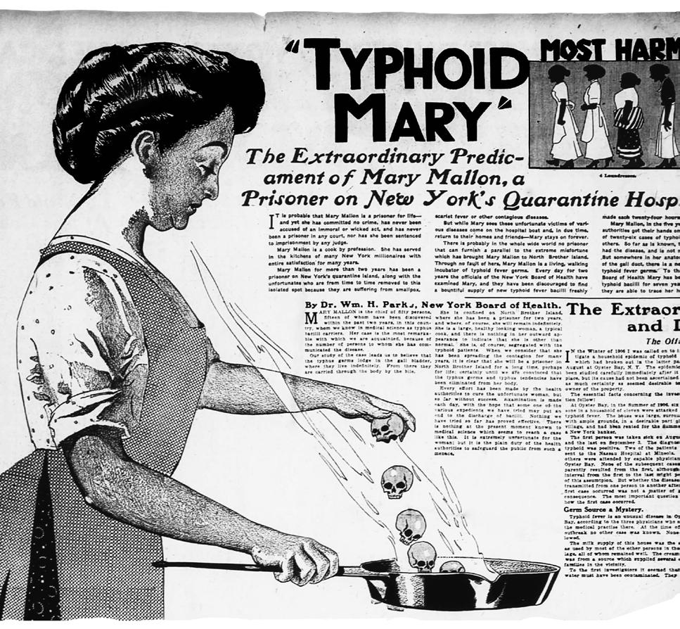
A famous case of a super-shedding individual is that of Mary Mallon – later known as “Typhoid Mary” – who unknowingly spread typhoid fever to an estimated 122 people. Caused by the Salmonella typhi bacteria, Typhoid fever is an infectious disease of the intestinal tract, which is typically transmitted via contaminated objects and food as a consequence of insufficient hygiene. Importantly, S. typhi goes through “showers” where asymptomatic hosts periodically release a large volume of the bacteria in their stool. Mary was an Irish woman who emigrated to the US at
Normal infected individual
Normal infected individual
Super-shedding individual
FIGURE 2.11 | Super-shedding individuals expel higher amounts of infectious material. Supershedding is thought to be due to components of the pathogen’s transmissibility and/or infected host characteristics, i.e. immune response.
Super-shedding individual
the age of 14. In 1906 she worked as a cook in a rental house and served food to eight families, seven of which eventually fell ill with the disease. At the beginning of this typhoid fever outbreak, investigators suspected the soft clams the families had eaten as the source of contamination. However, after learning that some of the ill patients had not eaten the clams, investigators realized there must be another cause. Later, it was determined that Mary Mallon was a “healthy carrier” who, despite only presenting very mild symptoms, had spread the disease around her, resulting in the death of at least five individuals. Mary was forcibly quarantined for a total of 26 years – far longer than our current understanding of the disease would recommend. Since then, the term “Typhoid Mary” has taken on a pejorative quality, cruelly implying that a person is reckless in regard to the health of others. Years later, many other healthy carriers of Salmonella typhi, like Mary, were identified.
As we’ve seen, no single number, rate, or tool can paint the full picture of an epidemic. Understanding these values in context of one another, in addition to how they relate to population size, geographic area, socioeconomic status, and any number of additional factors, can help us interpret a raw number like R0, and predict the spreading of a disease. Thus, it is important to adopt
Stop to Think
1. How do prevalence and incidence differ?
FIGURE 2.12 | Local newspaper featuring Mary Mallon as “Typhoid Mary.” The stigma towards Mary Mallon as the first identified healthy carrier of Salmonella typhi in the US gave her the name of “Typhoid Mary.” She is considered as the primary source for the 1907 typhoid outbreak in New York in which over 3,000 citizens were infected with the bacteria. Modern understanding appreciates that her treatment – by both public health officials and many of those who tell her story – was cruelly excessive and unethical. Of note, while this newspaper illustration implies transmission via breathing on the food she is preparing, we now understand that S. typhi is spread through fecal contamination.
an interdisciplinary approach, incorporating data and analytical methods from a number of different fields to build a comprehensive picture of disease and its impact.
2. If a disease has a high case fatality risk and a high prevalence, what might that tell you about the disease’s progression?
3. What are some possible reasons for excess mortality during an outbreak?
4. How does the reproduction number help predict the spread of a disease?
5. What is the “magic” number epidemiologists often hope to keep R0 below?
2.4: Data Collection and Study Design
We’ve discussed how epidemiology is founded on data from a wide range of scientific sources and some ways to interpret the data, but how exactly is that data collected? More importantly, how do epidemiologists even know what kind of data they will need to collect? When an epidemic is tearing through a community, experts must sort through a lot of information to fully understand the issue and devise a solution. As epidemiologists investigate the spread of disease across populations of people, they need to know what they’re looking for, and it all starts with the questions they choose to ask. There is a general protocol that epidemiologists follow to answer those questions with the design of a study; let’s look into it.
Hypothesis Design
The foundation of any successful scientific pursuit is a sound hypothesis. The hypothesis is a predicted answer to the research question. Much like how John Snow suspected that the Broad Street pump was the central culprit of the 1854 cholera epidemic, epidemiologists should already have enough familiarity with the situation to have an educated guess as to what the solution may be.
In science class, you may have already learned that a hypothesis can look like an “if… then…” statement that predicts the outcome of an experiment: “If a certain event occurs, then a specific effect will follow.” Similarly, epidemiologists use their hypotheses to explain how they think a certain phenomenon occurs.
A good hypothesis states a clear, testable relationship, such as a potential link between exposure and the disease. The hypothesis
should be limited in scope so that the researchers can distinctly isolate a singular observation and outcome without having to account for several other potentially impactful factors. Alluding to the earlier example of cholera and John Snow, an example of a hypothesis would be “if people no longer drink the water from the Broad Street pump, then the number of cholera cases will drop.” Just as John Snow based this hypothesis on the evidence he had collected pointing towards the pump as the source of infection, a hypothesis should also be consistent with known facts and supported by scientific literature or theories from other experts in the field. A researcher’s hypothesis will not always be correct, but it should always be a reasonable, informed guess based on the available information.
An important component of hypothesis development is the establishment of a null hypothesis. The null hypothesis states what will happen if the variables or populations under study do not have a significant relationship or difference between them. Essentially, it is the scenario we’d like to disprove. In the Broad Street pump example, Snow’s research hypothesis was that disabling the pump would curb the spread of cholera. His null hypothesis — assuming that the water from the Broad Street pump was not responsible for the cholera spread — would have been that disabling the pump would not affect the rate of cholera spread.
Research Methodology
Next, epidemiologists need to find a way to test this hypothesis. Ensuring that you are collecting the right kind of data is a science unto itself, known as research methodology. When investigating public health issues, epidemiologists are often in close
communication with community governments, industry leaders, healthcare practitioners, public health agencies, and hospitals in the local area to take advantage of existing data sources, or to perhaps design collaborative experiments and collect or generate new data. Epidemiologists need to consider many factors, including the population they aim to study, the intended sample size of the testing group, recruitment methods for study participants, data collection procedures, and confidentiality, and assess how each of these factors will help them to better understand their phenomenon of interest. There are many different types of studies to choose from, and the researchers must tailor their approaches to the specific types of data they plan to collect and analyze.
Types of Studies
Epidemiologists and other researchers frequently need to design ways to collect a large volume of reliable, high-quality data. Although they would ideally collect data from the entire population under investigation, such a process would be very challenging, and ultimately usually infeasible. Instead, they aim to find ways to study a sample of individuals as representative of the entire population as possible to retrieve applicable data in a more efficient manner. If collected well, the insights of this data should be applicable to the larger population of interest. Below we’ll describe study designs that are frequently used by epidemiologists, but are also widely used in other fields as well.
A retrospective study is when epidemiologists use existing datasets to answer their question, i.e. using data that was collected in the past to answer a new question. These types of data sets may include mortality statistics, hospital records, and even data collected as part of
previously conducted research projects. In the context of infectious disease outbreaks, retrospective studies can inform us about how previous outbreaks started and spread, or tell us more about the people who are most likely to become ill. Although there are benefits to utilizing existing data, including cost and convenience, using existing records has its own drawbacks. For example, the epidemiologists working on this new research project do not get to select their variables of interest in the dataset or add any additional individuals to the study. Additionally, past data cannot give great insight into the efficacy of a new intervention or technology, and ethical review committees may have placed limitations as to when and whether existing data may be used by different researchers.
In a prospective study, a group of individuals are chosen and observed over a defined period of time, with researchers documenting how their specific exposures impact their health outcomes going forward. Through frequent follow-ups, and by grouping the test subjects according to their relevant exposures, the researchers can better understand how and why specific factors impact certain health outcomes.
Prospective studies can be further classified as either observational or experimental. In an observational study, an epidemiologist divides individuals into groups depending on their exposures to a certain risk factor. The individuals within each respective group are ‘observed’ or monitored over time to see whether or not they develop the outcome of interest. For example, a researcher may take note of kids who grew up with a pet in their home versus kids who didn’t, and see how many individuals in each group develop allergies later in life. Most importantly, the researcher does not impose a treatment (or
Research question we want to investigate
Are we collecting new data or using preexisting data?
Pre-existing
PROSPECTIVE STUDY
Retrospective study
Do we want to change specific exposures or simply watch various outcomes unfold without intervention?
Experimental study Observational study
FIGURE 2.13 | A flow chart detailing how researchers may choose which type of study to employ. Note that experimental and observational studies are both types of prospective studies, but they differ greatly regarding how they collect data.
exposure) — in the case above, the researcher will not ask half the families to get a cat and tell half the families that they cannot have pets — instead, the research team just observes the outcomes of families that already fit the specified parameters.
In an experimental study, epidemiologists impose different conditions they aim to test on distinct groups in order to generate results for analysis. For example, researchers would randomly split the participants into groups and then instruct one group of subjects to perform regular exercise while telling the other group not to exercise for a few weeks. The epidemiologists then document the differences between each group’s respective fitness outcomes. Based on these outcomes, the investigators may be able to determine if the specific exposure being studied, such as regular exercise, was a direct
cause of the observed outcome — in this case the subjects’ level of fitness. It is important to recognize that experimental studies can be very difficult to perform in the realm of infectious disease, as it would be immoral to intentionally put study participants at risk of contracting an infectious disease in most settings.
Bias and How To Avoid It
As with any discipline involving study design, data collection, and data analysis, it is remarkably easy to accidentally build statistical biases and errors into epidemiological studies. Bias is a systematic error, meaning there is no mathematical or analytical way to “fix” the problem, as the structure of the experimental setup is flawed. Therefore, it is crucial that researchers design their studies to protect
against bias at the outset, and continue their careful work to avoid biases when executing their studies and analyzing their results.
Types of bias include observer bias, which occurs when a test subject’s behavior is altered simply because they know they are being observed, like how feeling pressure from your band instructor during an audition might cause you to miss a few notes you otherwise would’ve nailed. Another common type of bias is selection bias, where the subjects selected for a study were not actually selected randomly when they should have been – like studying average shoe sizes in New York City, but only using data from the Brooklyn Nets basketball team.
A subset of selection bias which can be conscious or unconscious, and one of the most societally harmful factors that can limit the scope and overall value of a study’s results, is racial bias. Research that is not inclusive of different racial groups might not be applicable to them in the long run, thereby perpetuating racial health inequities. As a result of racial bias in research, health professionals may not be able to apply the conclusions found to the population at-large. It is crucial to understand that different racial and ethnic groups have been significantly disadvantaged by both social and environmental factors that can impact their medical histories for generations to come. This information is extremely relevant to epidemiologists tasked with understanding the complex health states of a population. When traditionally underrepresented groups are neglected in this research, larger medical inequalities can surface and cause deadly misconceptions. Gender bias is a similarly problematic and frequently occurring risk in research, with many studies focused solely on diseases common among cisgender men, to the exclusion of other gender identities (Figure 2.14).
UNCONSCIOUS BIAS
FIGURE 2.14 | Unconscious bias. It is extremely important for researchers to be careful to avoid biases when designing studies, as well as collecting their data and forming their conclusions. Biases, including racism, sexism, discrimination, etc. can be imprinted in our brains and be conscious or unconscious. Therefore we need to continue to work in ways to reduce these systematic errors when designing research projects.
Correlation vs. Causation
Epidemiological data in particular is quite intricate, with infinite connections between biological, societal, and environmental factors that all work in tandem to impact our lives. All of these factors are known as variables (elements or features that can vary). Independent variables are factors that are not influenced by other variables within the study. Dependent variables are expected to be influenced by other factors of the study, more specifically by the independent variables. For example, the independent variable of increasing age increases the risk of developing many diseases: the dependent variables in this scenario. Given the complexity of relationships between many health variables, it is crucial that epidemiologists strive to not only limit the number of potential variables at play during the hypothesis, methodology, and data collection stages, but also remain mindful of unaccounted factors during the analysis stage — even with all the data collected, they may not always have the full picture.
One key concept to understand when we identify interesting relationships in research studies is that correlation doesn’t equal causation. Correlation is defined as a detectable relationship or association between two variables, whereas causation indicates that changes to one variable directly causes changes in the other variable(s) of interest. In saying that correlation does not always mean causation, we mean that merely seeing a relationship between two variables (e.g., shoe size and basketball aptitude) does not imply that one causes the other. Many other forces could be at work, and a correlational study is inherently not set up to observe those other factors.
One key reason that correlation does not always mean causation is due the presence of confounding variables: variables that influence the exposure but are also a risk factor for the
CONFOUNDER
FIGURE 2.15 | Confounding variables. In the setting of disease epidemiology, confounding variables affect both the exposure and the outcome. Confounders are both associated with the exposure of interest, as well as a risk factor for developing the disease of interest. These confounders may cloud true relationships, making it appear that the exposure is the direct cause of the disease when in reality, the confounder is responsible for the observed changes in both. It is particularly important to be on the lookout for confounding variables, as they are frequently not accounted for in a given study. This diagram shows the relationship between the exposure and the outcome and how they both associate with a confounder.
disease being studied, as shown in Figure 2.15. These variables may not have been noticed or accounted for during the experimental design process, but are directly associated with both the dependent and independent variables observed by the study.
A famous example of confounding can be seen in the classic example that ice cream sales and murder rates are very closely correlated. Even with this strong correlation or perceived relationship, it would not be accurate, nor useful from a public health perspective, to clamp down on ice cream sales in order to reduce homicides. Instead, this relationship implies that there is another variable at play that relates to both of these outcomes: namely stifling temperatures that lead to heightened emotions, and ice cream cravings. In this case, the true causative factor might be soaring temperatures, but the correlation alone does not give us enough evidence to make that conclusion and might even obscure the real underlying relationships if not interpreted carefully.
One way to mitigate bias is through randomization, the process of randomly assigning participants to different study groups. Randomization aims to limit the influence of individual characteristics on the study outcome. This way, participant characteristics that might influence the study outcomes, like gender, socioeconomic status, and many others, would be split evenly between the study groups, and their effects would be equal between both groups, and therefore have no effect on the outcome of interest between groups. In this way, any observed variation can be assumed to be a function of the treatment. In the case of our exercise study example, if all the individuals assigned to exercise were in their 20’s, while those told to refrain from
exercise were recruited from the local nursing home, clearly age would have a direct effect on how physically fit the two groups appeared to be after the experiment. Randomization aims to reduce the likelihood of these uneven distributions.
Equity and Ethical Conduct of Research
Ethics must be at the core of all research initiatives, particularly those in the realm of public health. Ethical studies not only treat participants with respect and autonomy during the study itself, but also ensure that the benefits of research are equitably distributed.
There have been egregious examples of unethical research practices in uncomfortably recent history. An infamous example was the Tuskegee Syphilis Study, run by the US Public Health Service and CDC from 1932 to 1972. The study was designed to observe the progression of syphilis in black men, despite the fact that the disease’s progress was already well documented (Figure 2.16). Black men were enrolled in the study, but not told that they had syphilis, endangering them, their sexual partners, and any children that were conceived after infection. More shockingly, participants were never told that in 1943 penicillin had become a highly effective, relatively simple and standard treatment for syphilis. The study instead went on for another 29 years, and many participants died of a curable disease.
Safeguards have since been placed in order to reduce the likelihood that such unethical studies are conducted. Nowadays, most research entities have Institutional Review Boards (IRBs) and Research Ethics Committees (RECs); these groups review and either approve
FIGURE 2.16 | Blood-draw during the severely unethical Tuskegee Syphilis Study. This study was designed to document the already well-known discourse course of syphilis, and was conducted without the consent of Black men in Tuskegee, Alabama. They were not told that they had syphilis, risking the health of the men themselves, their sexual partners, and any resulting children. Further, they were barred from accessing treatment when it became available.
or propose changes to research studies that are carried out by the institution before the study can begin. They are charged with protecting participants from harm, and as a by-product, protecting the public’s trust in human research.
However, ethics goes beyond just treatment of study participants. Public health initiatives must always strive to deliver equitable results. There are multiple ways that this needs to be achieved. The first is to ensure that research participants are reflective of the general population, or at least the population that would benefit from its results. For example, the results of studies that don’t have proportionate representation of particular ethnic groups may not be applicable to the groups excluded, placing them at risk for worse health outcomes down the line.
Another key component is to ensure that the communities that participate in the research
benefit from its findings. For example, it would be unethical to conduct a trial of a new pharmaceutical drug in a low-income community that could not afford to purchase the drug when the study is over. One way to achieve this aim is to include community members at every single step of the study’s conception, design, implementation, and analysis, and to reflect about the ethical considerations and implications of unethical research.
Engagement with community members will not only help ensure ethical research conduct, but will also increase the efficacy of the study, as it will help researchers understand the social and cultural norms that exist, and may pose barriers to uptake. For instance, it would not be a very good experiment to administer meat as a nutritional supplement among a group of people who are vegetarian, and questions about alcohol use might need to be handled differently when asked of different communities.
Studies must also be targeted towards reducing health disparities, i.e. differences in health outcomes between groups. For example, breast cancer rates and breast cancer mortality are significantly higher among black women than among white women in the US. Researchers have been conducting epidemiological studies to better understand the drivers of this difference, which include various social and environmental factors. Importantly, these studies both establish a baseline against which public health officials can measure progress, and can help identify appropriate interventions or treatments.
Epidemiologists are cognizant of the social determinants of health, or how aspects like race, gender, economic status, and other nonbiological factors, impact health. Tuberculosis is famously referred to as a ‘disease of the poor’
and recent research suggests that effective treatment not only requires appropriate pharmaceutical and clinical interventions, but also care for the social aspects of the disease. You’ll learn more about these sorts of social tors that affect illness in Chapter 10: Social Determinants of Health. The next step in working towards equitable health care is collecting high-quality data.
Data Collection
Having determined their epidemiological question, and thoughtfully planned out how they will choose test subjects and gather data, researchers must then collect the information they need. For John Snow, this data included the symptoms of the disease, personal accounts of individuals who witnessed the outbreak unfold, and – crucially – the locations of cholera-infected households. Researchers may also seek out specific environmental factors that may relate to the disease at hand, like air quality, the medical histories of infected individuals, or biological samples.
There are a number of different types of data, frequently split between qualitative and quantitative. Quantitative data can be measured in numerical units, while qualitative data are non-numerical, descriptive information relating to characteristics and attributes. Whether or not an epidemiologist will want to collect one form of data over the other, or both forms of data together, depends on the nature of their study and the questions they hope to answer. For example, an epidemiologist interested in the impact of COVID on one’s ability to breathe could collect quantitative information such as test subjects’ respiratory rates and the precise levels of oxygen dissolved in their blood, or
they could collect qualitative data, through asking participants to describe their shortness of breath, or even just their binary answer to the question “do you feel out of breath? Yes or No”. In doing so, they help to paint the clinical picture of the disease, and are able to describe key information like health outcomes and exposures. Increasingly epidemiologists, and scientists broadly, are recognizing the need to include both quantitative and qualitative data in research to better capture the full spectrum of outcomes.
Data Analysis
Once all the data is collected and the experiment is over, epidemiologists need to find ways to make sense of it. From their data, epidemiologists must identify trends and patterns to unearth the underlying story. During outbreaks, this process frequently involves synthesizing many different complex kinds of information including; the number of people who have been infected; their symptoms; their health-outcomes, and many others. This vast amount of information must then be processed and synthesized for further analysis and understanding.
As we noted above, there are many key metrics we can calculate, such as incidence, prevalence, risk ratios, and more. One key way to interpret the importance of these results is running tests of statistical significance You may have encountered significance tests such as Chi-squared tests, T-tests and Z-tests in your previous math and science classes. Statistical significance helps researchers assess the likelihood that their observations arose due to chance alone. In other words, the statistical significance assesses whether the null hypothesis is true and any variation in the data is due to chance, or whether there is likely to be underlying difference(s) between
the groups that the study is comparing. While the specifics of different statistical significance tests are outside of the scope of this textbook, it is important to realize that the likelihood of finding a significant result depends on the strength of an association, as well as the sample size of the study.
Statistical significance is critical to our understanding of outcomes and helps researchers identify what components of their data are both reliable and accurate, and thereby good foundations for potential interventions. It also helps root out some of the misinformation that often emerges in the chaos and fear of outbreaks.
Also important is the clinical significance of a finding, the impact it has on patient care. For example, let’s say that pharmaceutical developers find a new antibiotic that is proven to shorten patients’ duration of an ear infection in a statistically significant way. On the surface, this sounds like an incredible finding. However, let’s say that it was only shown to shorten the ear pain by one minute. Even though this finding reached statistical significance, and the drug shortened the patients’ symptoms, this one minute likely has limited — if any — clinical significance.
Conversely, a drug might have clinical, but not statistical significance. For example, let’s say that a new antiviral was developed. Even if it hasn’t been shown to statistically significantly reduce the length of the patients’ illness, it still has clinical significance if it is more tolerable to the patient, i.e. has fewer side-effects, or needs to be taken fewer times per day.
Another critical data analysis tool is the model , which is a more basic mathematical representation of a complex system that can be used to explain or even predict the
larger system’s features. Models are useful in many ways; notably, they can tell you what a certain piece of data may mean in the context of a greater phenomenon. For example, although R0 is a useful metric on its own, one of its primary functions is to be included in the susceptible, infected, and recovered (SIR) model, a relatively simple model of the spread of disease throughout a population. Using R0, as well as a few other basic pieces of information regarding the sizes of various groups in the population, can help map out the number of people susceptible to a disease, infected, and recovered at different points in time; with these small sample sets of data, we can build models like this one to draw population-level conclusions. You will learn more about modeling and SIR models in Chapter 13: Mathematical Modeling.
Visualization , or visual representations of the gathered information, is usually presented in tables, plots, diagrams, and graphs, which facilitate the comprehension and interpretation of research outcomes. These ways to illustrate data can display large amounts of information and even help identify the greater trends that may not have been comprehensible or apparent on a sheet of discrete, numerical data points. By graphing data or even simply organizing it into a table, it becomes much easier to see the connections within the data, and understand how it all may fit together.
Communication
Along with strong data collection and analysis skills, epidemiologists must be able to convey their findings to the relevant audiences. To a greater degree than other scientific disciplines, the work of epidemiologists is directly related to and affected by the actions and behaviors of
the general public. When a new discovery is made or a nuance is clarified, epidemiologists must present their work in a way that is understandable to the audience they aim to engage.
While this sounds straightforward, it can actually be quite complicated; some epidemiologists need to communicate only with other experts in their field, whereas others may need to inform anyone from elected officials and policymakers to front-line workers, private businesses, and the general public, all of whom have different backgrounds and priorities. Nowadays epidemiologists are even regularly speaking directly to people in the media and even in social media platforms like twitter and tiktok. It can be difficult to communicate a common message to each audience, but through data analysis tools such as the metrics, statistical significance, models, and figures we discussed, as well as their direct relationships to public policy, epidemiologists can clearly communicate their work in a way that enables correct interpretation of the science.
The audience is also important to have in mind when considering to whom the results might apply. For example, a study of methods to help reduce water-borne infections in some areas of the US may need to focus on stopping kids from swimming or playing in untreated bodies of water, whereas initiatives to reduce water-borne infections in under-resourced settings might be more tailored to education about water boiling and safe food preparation practices.
Another component of clear, accurate, and applicable communication is acknowledging our limitations. We should be clear in our communication that no study or experimental result will ever be perfect, and we must
always communicate openly about what we don’t yet know or are unsure about. It is also important to remember that although scientists often communicate in technical and nuanced terms, ultimately the goal is to help individuals and communities live healthier lives.
Stop to Think
1. Explain the relationship between a hypothesis and a null hypothesis.
2. Name two of the four types of studies described in this chapter, and give an example of a disease or health condition study you’d try to track using each type.
3. Why is it particularly important to adhere to ethical conduct of research?
4. What is a real-life example of correlation not implying causation? Be creative!
Stop to Think Answers
2.1: Introduction to Epidemiology
1. John Snow discovered that water was the source of contamination and that the disease causing the outbreak (cholera) was propagated through contaminated water (waterborne). John Snow’s contributions, although perhaps not as original as history credits him with, changed the future of public health by demonstrating the usability of maps for contact tracing, and the efficacy of datainformed interventions.
2. Spontaneous generation – later disproven – proposed that living organisms causing disease could arise from inorganic matter. Germ theory proposed that disease was passed by seed-like germs.
3. Germ theory helped the public appreciate the communicable nature of diseases, and focus their attention on effective interventions.
4. Modern-day applications include the development of effective outbreak response protocols, such as wearing masks in public, and social distancing.
2.2: Epidemiology Concepts and Definitions
1. Who: who was infected?
What: what were the symptoms, course of illness, and ultimate diagnosis?
When: when did the person fall ill?
Where: where was the person before, during, and after their illness?
Why: why did this person fall ill? (e.g., risk factors, activities, potential causes, exposure to other infected people, etc.)
2. Answers may vary but what’s important here is to make sure the concepts are well understood and can be translated into a real scenario. For example:
Case: Student from the local High School falls ill and presents symptoms such as a fever, sore throat and a headache.
Case Investigation:
• Who was infected? A student from the local High School
• What were the symptoms, course of illness, and ultimate diagnosis? Symptoms were noticeable enough that the student made the smart decision to not go to school and stay home to recover. The symptoms continued for two days, then they decided to call their care provider who suggested a flu test. Student tested positive for the flu.
• When did the person fall ill? On Monday
• Where was the person before, during, and after their illness? The person attended a school event on Saturday and went to swimming practice on Sunday.
• Why did this person fall ill? Most likely because this person attended a big event in which an infected person happened to spread the disease.
Exposure: The student attended their school event and swim practice, later learning that several students felt ill with a respiratory disease.
3. Asymptomatic transmission is the ability to pass the disease on to others while showing no signs of being sick. This is a big threat as patients carrying the disease may not be aware they are infected, and continue with their regular lives, spreading the disease within the community, and potentially sparking an outbreak. Another threat posed by asymptomatic transmission is the challenge in identifying and documenting such cases which affects the understanding of a disease, limiting protective public health measures.
2.3: Epidemiology Calculations
1. Prevalence tells us the number of active cases at a given time, whereas incidence tells us the number of new cases over a period of time.
2. A high prevalence with a high case fatality risk tells us that many people are getting sick and that many are likely to die once infected. Maintaining a high prevalence with a high case fatality rate indicates a very high replacement rate for those who die with newly-ill individuals.
3. Possible causes of excess mortality might include overwhelmed hospitals, closure of primary care services, self-medication with toxic substances, and many others.
4. The reproduction number tells the average number of people whom a single case is expected to pass the disease on, indicating the approximate spread expected.
5. Epidemiologists hope to keep R0 below 1 to avoid exponential spread.
2.4: Data Collection and Study Design
1. A hypothesis states what the researchers expect the outcome of the study to be. The null hypothesis describes what the outcome would be if the variables or populations of interest do not have a significant relationship or difference.
2. We discussed four types of studies in this chapter
a. Retrospective studies could be used to calculate the prevalence of the 1918 Influenza from existing records.
b. A prospective study could be established to calculate the incidence of COVID-19 in middle-school classrooms after vaccine administration.
c. In an observational study, researchers would split the groups by naturallyoccurring characteristics that they can observe. For example, epidemiologists may compare whether people who walk to work or drive to work have lower blood pressure.
d. In experimental studies, the “treatment” is imposed. For example, researchers might give half their study’s families a humidifier and compare whether the humidifier group or the no-humidifier group have more colds.
3. Answers will vary, but should include a discussion of ensuring the dignity and autonomy of participants, as well as ensuring that research is reflective of the general population, and ensuring that the benefits of the study are conferred equitably.
4. Answers will vary, but may include relationships like the following between per capita mozzarella consumption and civil engineering doctorates awarded.
PER CAPITA CONSUMPTION
OF MOZZARELLA CHEESE
Glossary
Asymptomatic Transmission: Manner of transmission when an infected individual presents few to no symptoms of the disease but is still contagious.
Bias: A study design error made by a lack of inclusion and/or prejudice for or against something or someone — frequently against particular groups of people.
Case: An instance of disease or outcome of interest.
Case Definition: The naming of factors that must be present in order to consider any given observation a case.
Case Fatality Rate (CFR): The proportion of individuals with a disease in a population who die from that disease during a specified time period; also known as case fatality risk or case fatality ratio.
CFR = # of Individuals who died from disease in specified time period / Total # of individuals in population with disease at time
# of cases who died from disease in specified time period
Total # of cases with disease in specified time period
Case Investigation: When epidemiologists employ tools to identify and classify instances of the disease in a population and develop a better understanding of its characteristics at the individual and/or community level.
Causation: Indicates that changes to one variable directly causes changes in the other variable(s) of interest.
Clinical Significance: The impact a statistical finding has on patient care outcomes.
Cluster: A grouping of cases in excess of what would be expected in that given area.
Confounding Variables: Variables that have a direct relationship to the variables under study, but are not accounted for in the study itself.
Contact Tracing: Documenting the social interactions and movement of an infected person in order to help contain an outbreak and better understand its spread, scale, and scope.
Correlation: A relationship or connection between two factors such that change in one is linked to (but does not necessarily cause) change in the other.
Epidemiology: The study of the distribution and drivers of health and health risks.
Excess Mortality: The difference between the observed number of total deaths in a population at a specified time period and the number of deaths one would expect in a ‘normal’ time period, often obtained from real-life data of the same population during times of non-crisis.
Excess Mortality
# of deaths in population during this time period
# of deaths in population in a ‘normal’ time period
EM = # of deaths in population during the time period – # of deaths in ‘normal’ time period
Experimental Study: A study in which the investigator directly impacts the properties of each group.
Gender Bias: Attitudes towards others or associated stereotypes towards people of different gender identities; can be implicit, meaning these are unconscious biases in favor
of or against others, without our conscious knowledge. Many studies focus on cisgender men, excluding people of other gender identities.
Geolocation: Tracking the places with which infected individuals have interacted using geographic information sciences (GIS) systems and software.
Germ Theory: The theory that infectious disease is transmitted by small “seeds” that could be passed between people and contaminated objects.
Hypothesis: A predicted answer to the research question you are posing.
Incidence: The number of new cases within a population over a given period of time.
Incidence Proportion: The frequency of new cases of the disease within a certain population over a specified period of time.
Incidence Proportion=# of new cases during the given time interval# of susceptible people at the beginning of the time interval
Index Case: The first case identified by health officials in an outbreak (colloquially known as “patient zero”).
Model: A more basic mathematical representation of a complex system that can be used to explain or even predict the larger system’s features.
Mortality Rate: Represents the entire susceptible population’s risk of dying from a disease, not just those infected with the pathogen.
Mortality Rate= # of deaths from diseaseTotal population susceptible to disease
= # of deaths among cases due to disease
Null Hypothesis: States what will happen if the variables or populations under study do not have a significant relationship between them.
Observational Study: A study in which an epidemiologist divides individuals into groups depending on their exposures to a certain risk factor. Over time, the individuals within each respective group are tracked to see whether or not they develop the outcome of interest.
Observer Bias: When a test subject’s behavior is altered simply because they know they are being observed.
Overdispersion: A statistical phenomenon in which a small group of infected individuals is responsible for a large percentage of infections, rather than every infected individual contributing to the spread equally.
Overdispersion Parameter (k): Describes individual variation in disease spread. Smaller k values indicate that a small number of individuals make big contributions to disease spread, whereas larger k values indicate more equitable spread by a larger number of individuals.
Person-years: A unit of measurement that reflects the total amount of time that study participants were observed. For example, if a study that has 100,000 participants, and lasts for one year, that is 100,000 person-years of observation. A two-year study with 50,000 participants would also have 100,000 personyears of observation.
Prevalence: How many current cases of a certain disease there are in a population at a given time.
Mortality Rate x 100
Total population susceptible to disease
Prevalence= # of existing cases at the given time Population size at the given time
Prevalence=# of existing cases size at that timePopulation size at that time
Primary Case: The individual who first brings a pathogen into a specific population; this individual frequently goes unidentified.
Prospective Study: A study in which a group of individuals are chosen and observed going forward, with researchers documenting how their specific exposures impact their health outcomes in real time.
Proximity Sensing Technologies: Technologies that can automatically catalog interactions between individuals by using their geographic location information from smartphones and Bluetooth technology, etc. Used for contact tracing.
Public Health Surveillance: The systematic collection and analysis of population-level health data.
Qualitative Data: Any data that is nonnumerical and/or descriptive; relating to characteristics and attributes.
Quantitative Data: Any data that can be counted or measured in numerical units.
Racial Bias: Attitudes towards others or associated stereotypes towards people of different racial groups; can be implicit, meaning these are unconscious biases in favor of or against others, without our conscious knowledge. Can perpetuate health inequities (i.e., research not being inclusive of different racial groups, drawing conclusions not applicable to the broader population).
Randomization: The random assignment of the intervention; randomly assigning participants to different study groups to mitigate bias and limit the influence of individual characteristics on the study outcome.
Reproduction Number (R): Describes the transmissibility of disease and has different variations depending on the population being studied.
Basic Reproduction Number (R0): Pronounced “R-naught,” the average number of new cases of a disease caused by a single infected person within a population that is fully susceptible to the disease.
Effective Reproduction Number (Rt): The number of new cases of a disease caused by a single infected person in a population that is only partially susceptible.
Research Methodology: The science of ensuring that you collect the appropriate data to answer a given research question.
Risk Difference: The difference between the incidences in a group exposed to a certain risk and an unexposed group with otherwise similar characteristics; also known as attributable risk or excessive risk.
Risk Ratio: Compares the risk of an outcome of interest among the exposed group to the risk among the unexposed group. It does so by dividing the risk in the exposed group by the risk of the unexposed group.
Risk Ratio=Risk of outcome of interest in exposed groupRisk of outcome of interest in unexposed group
Retrospective Study: When epidemiologists use existing datasets of previously-collected data to answer their question.
Secondary Cases: The cases of a disease caused by a single infected person.
Selection Bias: When subjects selected for a study were not actually selected randomly but should have been.
Social Determinants of Health: Aspects such as race, gender, economic status, and other non-biological factors that impact health.
Spontaneous Generation: The now-disproven theory that diseases and living organisms arose from non-living matter.
Statistical Inference: The study of data to make predictions about a phenomenon of interest.
Statistical Significance: Mathematical evaluation of the statistical likelihood that a given observation is due to chance alone; an indication that the exposure likely caused the outcome. Observations that are found to have sufficiently low likelihood of being due to chance are considered significant.
Super-shedding: A term applied to an individual who for a period yields many more infectious microbes than the majority of the same host species, meaning that many more infectious units are released than normal.
Superspreaders: Individuals who by virtue of biological or behavioral actions infect many people; for example, attending multiple events where they get in close contact with multiple individuals, infecting other attendees.
Superspreader Event: Occasion during which a small number of individuals (or even just one) pass a pathogen to a large number of people.
Transmission Rate: Describes the flow of individuals in a population going from a susceptible state to an infected state.
Visualization: Visual representations of information (e.g., data tables, plots, diagrams, graphs).