An Autonomous Vehicle at the Handling Limit: A Hierarchical Controller Based on the Quasi-Steady-State Model

Safe autonomous vehicles must be reliably controlled in many situations, including in transient on-limit manoeuvres, e.g. obstacle avoidance. Many control algorithms used for autonomous vehicle control are founded on linear vehicle dynamics and sub-optimal control models [1,2], and thus their application in extreme vehicle manoeuvring tasks is limited. The main challenges associated with on-limit vehicle control are two-fold: The prediction accuracy of the vehicle response within the environment, and the computational effort of the control calculations.

This work attempts to bridge the gap between the prediction accuracy of the vehicle modelling task and the real-time implementation of Model-Predictive-Control (MPC). This paper presents the formulation of a hierarchical control framework which capitalises on the advantages of both vehicle models. A path planning model is used to assist with optimal control refinement. Racing car lap-time simulations [3-8] are used in this work for result comparisons as they provide a convenient platform to assess the performance of the controller in transient onlimit manoeuvres. Future developments of this controller may be more suited to specific autonomous vehicle control tasks. This paper is organised as follows. Section 2 introduces the vehicle modelling techniques. Section 3 will outline the hierarchical control framework employed in vehicle modelling tasks. Section 4 shows the results of the research and Section 5 concludes the paper.

2. Vehicle Modelling

Three vehicle modelling formulations are presented in this section. The first is a geometric path planning tool which provides feasible trajectories to point mass minimum time problems. The second is a minimum time point mass vehicle model which accurately predicts vehicle behaviour in transient on-limit vehicle manoeuvring problems. Lastly, a short horizon 7 Degree-of-Freedom (DOF) transient vehicle model is used for path following.

The three models outlined in this section form a hierarchical control framework used to control a vehicle in minimum time manoeuvres. The unique contribution of each model is outlined in Section 3.

2.1 Path Planning

Most path planning tools employed in vehicle modelling tasks are geometric in nature, due to their computational speed. Geometric paths provide a robust method for determining time optimal solutions to the minimum time path. Minimum curvature paths are often the choice of geometric solution [9,10] as this closely resembles the minimum time path of a racing circuit. Vehicle trajectory curvature is also importantly related to the vehicle acceleration as the normal acceleration (an) can be determined with vehicle speed (V) and the curvature of the vehicle trajectory (Kv).

(1)

Abstract

Most approaches to autonomous vehicle control are focused on normal driving conditions and are not suitable for on-limit control due to the non-linear nature of on-limit behaviour. Situations which require on-limit control are also commonly constrained by hard boundaries and require fast computation times, providing a unique set of problem constraints that are challenging to fulfill.

Understanding the relationship between curvature and trajectory is therefore of fundamental importance. The curvature is presented in the global (inertial) coordinate frame.

(2)

When the monotonic derivative indicator ( ̇) is defined w.r.t. trajectory arc length (Sv), eq.(2) is simplified with a denominator equal to 1. Whilst this simplification assists with computational effort, the resulting equation remains within the global framework and therefore curvature resolution is still challenging. By evaluating the trajectory curvature in a curvilinear coordinate frame (track), a new equation for curvature is presented [4].

(3) where Dv is the vehicle reference line offset, Kv is the reference line curvature and Q is the vehicle to reference line translation ratio. of the velocity (e.g. braking at constant acceleration along SC) therefore provides conservative feasibility assessments of the motion along the path. The variables (DV, DV , an and jn) are then imposed as state/ control parameters in the development of the trajectory to determine feasible paths in a geometric format.

Numerical simulation of on-limit manoeuvres often carries significant computational burden, precluding the direct use of full transient vehicle simulations in Model-PredictiveControl (MPC). Quasi-Steady-State (QSS) lap time simulation is a modelling method commonly found in motorsports, which uses point mass dynamics to control a vehicle within a set of predefined acceleration and jerk envelopes. QSS models are capable of accurately predicting the transient velocities and trajectories of on-limit vehicle motions, though vehicle controls such as steering and throttle cannot be formally tended to with this method. This paper presents a 3-tiered hierarchical control framework used to control autonomous vehicles in on-limit handling based on QSS motion. A simple constrained geometric path evaluation algorithm is used to determine a feasible path for initialisation, with QSS free-trajectory optimisation used to determine trajectory and velocity profiles. Finally, a short horizon transient vehicle model optimisation is used to convert QSS motion into a set of autonomous vehicle controls. The controller is evaluated in a Model-in-the-Loop setup, where the ability of the hierarchical framework to control the vehicle in near realtime is demonstrated at the limits of handling. Vehicle response is compared with a fixed horizon transient and fixed horizon QSS optimal control model, providing favourable results.

KEYWORDS: Autonomous vehicles; Lap-time simulation; Quasi-Steady-State; Hierarchical controller; On-limit control.

(4)

Track variables Xc and Yc, and vehicle reference line offset Dv are fitted with piecewise polynomial splines to impose acceleration continuity across the path.

All are functions of the reference line arc length (SC).

The 2nd and 3rd derivatives of the parameterised eq.(3) are notably explicit forms of normal acceleration (an) and normal jerk (jn) if the velocity is known. Trivial developments

The state (XT) and control vectors (UT) are shown.

Equality constraints are calculated with state space derivative (XT ).

The track spline coefficients (c1 − c12) are developed during the environment mapping process and the reference line curvature KC is calculated directly with the numerator of eq.(2), employing track spline coefficients.

2.2 Point Mass Motion

The point mass vehicle model has only two DOFs and is controlled with planar jerk variables [3]. As the equations of motion do not consider the yaw degree of freedom, the only non-inertial reference frame available is the natural coordinate frame, which is fixed at the centre of mass and orientated in the direction of the path of motion [11]. Accelerations and jerks are therefore presented in the natural coordinate frame. The state (X2) and control vector (U2) for the point mass vehicle is shown.

The spatial derivative of an is.

The state derivative variables are presented.

As fixed distance problems require state space transformation, the spatial first order Runge-Kutta marching method is presented.

The state space derivative is.

2.3 Transient Vehicle Motion

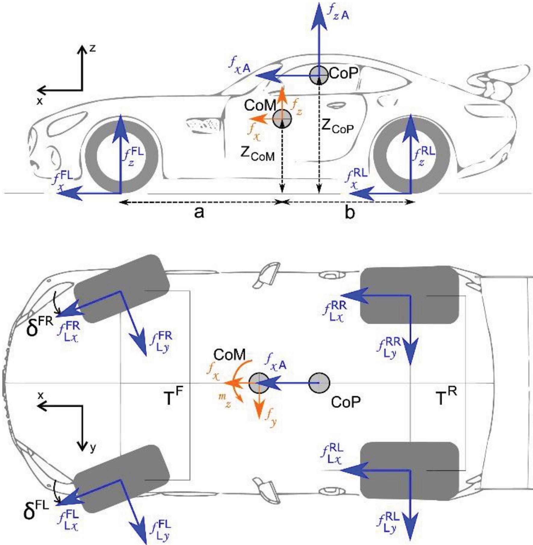
The transient vehicle model has two distinct developments, those are the rigid body equations of motion which apply to the general plane motion of the chassis (3 DOF) and driveline equations of motion which are used to determine the wheel state for tyre force evaluation (4 DOF). Development of the complete set of equations of motion is outside the scope of this paper, thus the authors refer the reader to [3] for the full development. The state vector for the transient vehicle model is presented.

Where YC is the yaw rate of the chassis, w j is the anular velocity of each wheel, and T, and 8 are the normalised throttle/braking and steering positions respectively. The control vector is presented.

(22)

The spatial marching method presented in eq.(18) equivalently applies to the transient vehicle model, as does the state space transformation eq.(19). The remaining transient derivative variables are developed via a summation of wheel and chassis forces and moments.

As the transient vehicle model forces are evaluated in the body coordinate frame, NewtonEuler equations of motion are presented.

(23) (24)

3. Hierarchical Control Framework

As the use of full transient vehicle models is too computationally costly for real-time MPC [12], a hierarchical set of vehicle modelling tools, fig.(3), is sequenced here to control the vehicle at the limits of handling. First, a feasible path planning method is used to develop a minimum curvature trajectory with horizon length SC = 500m. Next is a QuasiSteady-State (QSS) point mass model is used to predict the minimum time response of the transient vehicle model. The horizon length of the QSS model is SC = 300m and has an end state condition, DV and TOV defined by the feasible path planning model, which ensures that the end state of the QSS manoeuvring problem is positioned close to the minimum time solution, improving initial control refinement.

The last stage of the hierarchical controller is the restricted horizon length transient vehicle path following controller. The horizon length is only SC = 10m, with end state constraints defined by the position DV and heading angle TOV from the QSS vehicle motion problem. The optimisation objective minimises a mean-square of the QSS and transient velocity profiles along the trajectory. The short horizon distance of the transient path following controller allows the control algorithm to run in near real-time. It is expected that improvements to the controller, e.g. higher order explicit RungeKutta methods, discretisation refinement, or implicit solver implementation will significantly improve computation time [13,14]. The current method therefore demonstrates the utility and feasibility of the framework.

3.1 Feasible Path Planning Control

The path planning optimal control problem intends to provide minimum curvature paths. The minimum curvature path closely resembles the minimum time optimal control solution in a geometric format. Vehicle motion along the path is used as the QSS MPC initial guess. This initial guess is sufficiently close to the optimum for reliable solver convergence [4].

The cost function of the optimisation problem is shown as. (25) where the control segment is defined by (∆SU = 1m, : N = 500), and the analysis segment is defined by (∆SV = 0.05m, : n = 20). The permissible set of states and controls are determined by track and vehicle parameters. The trivial velocity profile is evaluated with constant reference line acceleration.

(26) representation of the maximum quasi-steadystate (QSS) accelerations of the equivalent transient vehicle model. The acceleration envelope development is outside the scope of works but is outlines in [3]. The acceleration constraint is imposed on the point mass motion problem as a non-linear inequality constraint.

Two acceleration envelopes are used in this work. The first is a Normal-TangentialAcceleration (NTA) surface [3], and the other is a friction ellipse (FE) surface (designed to match the NTA surface while remaining below to ensure control reliability).

A strategic set of jerk limits for this vehicle was also outlined in [4]. Appropriate jerk limits are one of the major driving factors behind the alignment of QSS and transient models.

Track position DV and track heading angle TOV are imposed on the QSS motion problem as an end state constraint and are derived from the feasible path planning solution at a horizon length of SC = 300m. The remaining permissible states are derived from track and vehicle parameters.

The minimum time cost for the QSS problem is presented.

Where the control segment is defined by (∆SU = 1m, : N = 300), and the analysis segment is defined by (∆SV = 0.05m, : n = 20). The formal optimisation problem for the QSS model is. (30)

The formal optimisation problem for path planning is.

3.3 Transient Path Following with Restricted Horizon Length

3.2 QSS Minimum Time Control

The QSS model is used to accurately predict the minimum time response of the vehicle. Improved computational efficiency of this simplified model provides a platform that is more suited to real time control.

The acceleration envelope that restricts the point mass accelerations is developed offline with an optimisation problem and is a

QSS vehicle motion is simplified to improve computational efficiency, but vehicle controls are untended. The receding horizon transient vehicle model, which does tend to controls, cannot be used due to its computational efficiency. Computational efficiency however, scales with problem size, thus the transient vehicle model can be used if the horizon length is sufficiently short (H<10m). Reliability of open loop vehicle control with reduced preview distance however, cannot be guaranteed. The transient vehicle model must therefore have strict end conditions which ensure its forward-looking reliability when horizons are short, turning the problem into a path following task. As the QSS point mass model can accurately predict the transient minimum time response, the strict end conditions placed on the transient vehicle model can be derived from here.

Consistent with the path planning and QSS vehicle models, the transient vehicle model is also restricted by a set of permissible states and controls. In addition to these, it is also beneficial to restrict sub-states, such as tyre slip ratios. Restricting tyre slip states reduces both tyre wear and the possibility of entering into unstable and/or unrecoverable vehicle manoeuvres, which is particularly important with short horizon lengths. These additional restrictions are presented in the optimisation problem as a nonlinear inequality constraint. (31)

Where k and k are the upper and lower bounds imposed on the slip ratios.

The objective function for the transient vehicle model is. (32)

Where w1 is the weigting factor applied to each analysis step, V(i) is the transient vehicle velocity, VQ(i) is the target vehicle velocity defined from the QSS minimum time solution. Where the control segment is defined by (∆SU = 1m, : N = 10), and the analysis segment is defined by (∆SV = 0.0125m, : n = 80).

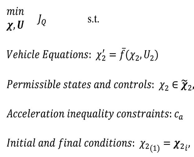
The formal optimisation problem for transient path following is.

(33)

The hierarchical controller can be simulated in the virtual space by using a vehicle model in place of the autonomous vehicle response where a virtual control loop is setup, referred to as Model-In the-Loop (MIL). Whilst this work employs identical prediction and control models (assuming a definite environment and accurate modelling), the MIL framework provides a platform for virtual validation of the control framework. Artificial implementation of response disturbance (through differences in precision and control modelling) will yield differences in the outputs of the models which can be used to assess the robustness of the controller. This is reserved for future work. Before proceeding to results, it is noted that the performance of the path following controller should not exceed that of the QSS full length minimum time solution as the target is only to follow both the path and velocity profile. Receding horizon solution should also be slower than the full circuit problem as global optimisation characteristics are not observed in the local minimum time response [15]. It is therefore hypothesised that the MIL simulations will have slower optimal times than the comparative works.

4. Results

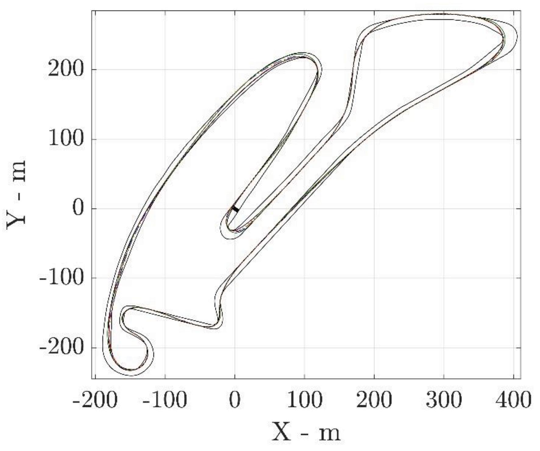
This work compares five simulations on the Tempelhof Airport Street Circuit (Berlin).

The first three are full length minimum time optimisations with transient and QSS models (NTA and FE). The last two are minimum time hierarchical MIL simulations (NTA and FE). Transient and QSS lap-time simulations are developed with the methods presented in [3,4] including all vehicle model parameters. The hierarchical controller presented in this paper also utilises identical vehicle parameters for comparability. The initial state of all examples is equivalent in their respective forms and are fixed. All simulations are implemented in MATLAB and are solved using the FORCES PRO NLP solver presented in [16,17].

The optimal trajectories are presented in fig.(4). The reference line orthogonal offset (DV), fig.(5), shows the trajectory of the QSS and MIL simulations. The deviation of those trajectories from the transient response is also presented in fig.(6). The trajectories presented show a good alignment of the transient response for both the QSS and MIL simulations. As the FE models have a regions in the acceleration envelope with largely different acceleration capabilities (due to the FE surface remaining exclusively beneath the NTA surface), large divergences between the FE and transient trajectory can be seen. The biggest difference in the trajectories of the vehicles occurs on the large sweeping left hand turn (circa SC ≈ 250m – 650m). In this section of the track, the racing line sensitivity to full lap manoeuvring time is low, so variability between the models is large.

The velocity states, fig.(5) and deviations, fig. (6), also show a good alignment however there is a clear distinction between the NTA and FE models here. Peak deviations of the NTA lap-time simulation velocities are within 1m/s of the transient vehicle as compared to the FE lap-time simulation which have velocity deviations beyond 4m/s. This is explained by the differences in acceleration surfaces. The hierarchical controller deviations are higher for their respective QSS models.

The track heading angle (TOV) also shows a good alignment. Notable deviations in the final hairpin, however, indicate a different mode of operation for the QSS lap-time simulations. This difference is not unexpected as when speeds are low (V<10m/s) the QSS vehicle model assumptions are less accurate. The alignment of the vehicle response is important in the evaluation of the controller capabilities. One of the most important evaluations to make is the alignment between the MIL simulation and the QSS lap-time optimisation for the same vehicle model. This comparison gives an indication to the performance of the transient path following controller. The relative comparison for NTA is +1.5% and for FE is 0.8%, which is slightly higher than the expected deviance due to the receding horizon effects. The direct comparison between the MIL (NTA and FE) and transient yielded a difference of +2.2% and +8.6%. Comparisons between the QSS and transient however are as expected at +0.6% and +7.8% respectively, thus the deficiencies in the MIL controller must be explained by deficiencies at the transient path following level.

When the MIL controller is entering a braking zone, the optimal jerks close to the current position (H<10m) appear not to align perfectly between the QSS and transient path following controller. This causes the velocity of the path following controller to overshoot the target QSS velocities. As the hierarchical control method is open loop, the overshoot cannot be recovered by the succeeding QSS model, resulting in a sub-optimal target path for path following. It is this overshoot that produces the comparative deficiencies of the MIL controller.

Noting this deficiency, the hierarchical controller still shows excellent control capabilities at the limits of handling. The local jerk sensitivities in the path following controller therefore provide an avenue for future work to incrementally improve both the QSS and transient alignment.

The piecewise NTA surface requires significant computational effort to compute which limits its real-time applicability. Comparatively, the FE model is much simpler and thus is much quicker to compute.

Normalised computation comparisons appear in Table 1, noting that the FE MIL controller is roughly one order of magnitude away from real-time implementation.

Real-time implementation of the control framework requires several improvements. Potential examples include refinement of the control and analysis discretisation, acceleration envelope discretisation, and explicit/implicit modelling formulations provide an additional avenue for further research.

5. Conclusions

Safe autonomous vehicles need to be accurately controlled in many situations, including in transient on-limit manoeuvres. High fidelity controllers are however too computationally expensive to run in realtime. QSS models solve this problem and are sufficiently accurate to predict the transient response, but vehicle controls are untended. A hierarchical control structure is presented in this work to solve these challenges. Results of two Model-In the-Loop (MIL) simulations are presented for comparison against QSS and transient lap time simulations. Comparisons of QSS and transient lap-time simulations are in line with expectations, however the hierarchical control model deficiencies are slightly higher than expected.

Deficiencies in the controller are explained by velocity overshoots from the transient model at the point of braking initialisation. This is caused by a misalignment of the local jerk characteristics in the local problem horizon (H<10m). As the MPC form is open loop, this results in sub-optimal QSS trajectories that cannot be recovered. Noting this deficiency, the hierarchical controller still capable of controlling the vehicle to a minimum time performance of +1.5% as compared to its maximum potential (defined by the QSS laptime simulation). The observed phenomenon provides an avenue for future work on the specification of the QSS jerk limits. The computation time of the hierarchical controllers is also assessed. It is noted here that the NTA surface model is more computationally costly as compared with the FE model. It is expected that refinement of the optimal control structure will bring the hierarchical controller with FE to be real time capable.

References

[1] N. H. Amer, H. Zamzuri, K. Hudha, and Z. A. Kadir, Modelling and control strategies in path tracking control for autonomous ground vehicles: a review of state of the art and challenges, Journal of intelligent & robotic systems, vol. 86, no. 2, pp. 225254, 2017.

[2] P. Falcone, F. Borrelli,E. H. Tseng, and D. Hrovat, On low complexity predictive approaches to control of autonomous vehicles, Automotive Model Predictive Control, Springer, London, pp. 195-210, 2010.

[3] K. Tucker, R. Gover, R.N. Jazar and H. Marzbani, A comparison of free trajectory quasi-steady-state and transient vehicle models in minimum time manoeuvres, Vehicle System Dynamics, 2021.

[4] K. Tucker, R.Gover, R. N. Jazar and H. Marzbani, Feasible Trajectory Planning for Minimum Time Manoeuvring, Submitted*, 2022.

[5] D. Casanova, On minimum time vehicle manoeuvring: the theoretical optimum lap, PhD thesis, Cranfield University, 2000.

[6] D. P. Kelly, Lap time simulation with transient vehicle and tyre dynamics, PhD thesis, Cranfield University, 2008.

[7] D. Brayshaw, Use of numerical optimisation to determine on-limit handling behaviour of race cars, PhD thesis, Cranfield University, 2005.

[8] M. Veneri and M. Massaro, A freetrajectory quasi-steady-state optimalcontrol method for minimum lap-time of race vehicles, Vehicle System Dynamics, vol. 58, no. 6, pp. 933-954, 2020.

[9] F. Braghin, C. Federico, M. Stefano, and S. Edoardo, Race driver model, Computers & Structures, vol 86, no. 13-14, pp. 15031516, 2008.

[10] A. Heilmeier, A. Wischnewski, L. Hermansdorfer, and et al., Minimum curvature trajectory planning and control for an autonomous race car, Vehicle System Dynamics, 2019.

[11] R.N. Jazar, Advanced Vehicle Dynamics, Springer, NY, 2019.

[12] R. Lot, N. D. Bianco, The significance of high-order dynamics in lap time simulations, The Dynamics of Vehicles on Roads and Tracks, CRC Press, pp. 561570, 2016.

[13] T. Novi, A. Liniger, R. Capitani and C. Annicchiarico, Real-time control for at-limit handling driving on a predefined path, Vehicle System Dynamics, vol. 58, no. 7, pp. 1007-1036, 2020.

[14] N. D. Bianco, E. Bertolazzi, F. Biral & M. Massaro, Comparison of direct and indirect methods for minimum lap time optimal control problems, Vehicle System Dynamics, vol. 57, no. 5, pp. 665-696, 2019.

[15] J. R. Anderson & B. Ayalew, Modelling minimum-time manoeuvering with global optimisation of local receding horizon control, Vehicle System Dynamics, vol. 56, no. 10, pp. 1508-1531, 2018.

[16] A. Domahidi and J. Jerez, FORCES Professional, Embotech AG, 2014-2019, url<https://embotech.com/FORCES-Pro>.

[17] A. Zanelli, A. Domahidi, J. Jerez and M. Morari, FORCES NLP: an efficient implementation of interior-point methods for multistage nonlinear nonconvex programs, International Journal of Control, pp. 1-17, 2017.