Cancerous Tumor Segmentation of Kidney Images and Prediction of Tumor Using Medical Image Segmentati

Research Article

Clinics of Oncology

ISSN: 2640-1037

Volume 4

Cancerous Tumor Segmentation of Kidney Images and Prediction of Tumor Using Medical Image Segmentation and Deep Learning Techniques

Akram Z*, Kareem MS, Mughal B, Ahmed Z, and Aziz S Department of Computer Science and IT, Faculty of Science, Khwaja Fareed University of Engineering and IT, Rahim Yar Khan, Pakistan

*Corresponding author:

Zaib Akram, Department of Computer Science and IT, Faculty of Science, Khwaja Fareed University of Engineering and IT, Rahim Yar Khan, Pakistan, Email: akram.zaib155@gmail.com

Keywords:

Tumor Detection Cancer; Kidney Images; Deep Learning; Modified CNNs

1. Abstract

Received: 11 Feb 2021

Accepted: 05 Mar 2021

Published: 09 Mar 2021

Copyright:

©2021 Akram Z, et al. This is an open access article distributed under the terms of the Creative Commons Attribution License, which permits unrestricted use, distribution, and build upon your work non-commercially.

Citation:

Akram Z, Cancerous Tumor Segmentation of Kidney Images and Prediction of Tumor Using Medical Image Segmentation and Deep Learning Techniques. Clin Onco. 2021; 4(2): 1-9.

Tumor Detection or Kidney Carcinoma Tumor is type of Kidney Cancer, which is very hazardous for health. There is a need of a proper analysis on this disease to treat the patients Kidney Tumor. Therefore, we have proposed an intelligent Tumor detection system. The main purpose of this research is to develop and implement an automated method that will help to detect and classify the Kidney Cancerous Tumor by processing Kidney images of Kits 19 dataset. We have used Kidney Tumor Segmentation dataset for testing our proposed methodology, it contains 300 CT-Scans images of Kidney Cancer patients. We have applied preprocessing techniques on these images such as morphological filtering, to enhance images. After obtaining the resultant image we have applied augmentation. We have used modified form of Convolutional Neural Network for classification purpose. The proposed technique provides a sophisticated diagnosis and 3 cross folds of prediction and validation loss with dice score and cross-entropy when compared with previous techniques. The parameter we used to validate the performance of our proposed technique is cross foldings, dice score and cross-entropy.

2. Introduction

The chief clinical application of kidney imaging comprises excluding rescindable reasons of acute kidney grievance, like urinary obstruction, or recognizing permanent Chronic Kidney Disease (Kidney Carcinoma) that prevents unnecessary diagnosis like

kidney biopsy [1]. Its noninvasiveness, little cost, lack of ionizing radioactivity, and wide accessibility make it a gorgeous option for recurrent monitoring and complement of the longitudinal variation in kidney dimension and sonographic features of kidney cortex related to kidney useful change. Though, the high individual variability in image gaining and clarification makes it problematic to interpret experience-based calculation into consistent practice, like invasive blood serum creatinine amount. Up till now, noninvasive imaging methods for organ practical and structural classification have been progressively investigated directing to diminish the invasive method in both problem-solving and screening situations. [2] has newly anticipated an inimitable pediatric Kidney Carcinoma maintenance model corresponding cost and minimizing incisiveness with the development of risk estimation by utilizing kidney CT imaging to predict the advance of Kidney Carcinoma and clinical conclusions in infants.

Conservatively, nephrologists lean towards kidney dimension, volume, cortical width and echogenicity to assess the sternness of kidney injury. Identical short renal measurement (e.g., <8cm), deceptive white cortex, limited capsule contour, entirely indicate a permanent kidney failing procedure with great specificity but restricted sensitivity [3]. Additionally, whether these scans parameters can be utilized to predict precise Estimated Glomerular Filtration Rates (eGFRs) remains argumentative. For example, [3][4] studies have described that even though kidney dimension is highly

detailed in detecting permanent Kidney Carcinoma, its association with eGFR was solitary week to modest, ranging no connotation to 0.66. Even, researches using the conventional modification diet in renal disease research (MDRD) equation to evaluation eGFR (MDRD-eGFR) are measured, the finest correlation well-known between kidney dimension and eGFR has been 0.36. Likewise, a fair-to-moderate association of kidney dimensions and cortical echogenicity through eGFR has been stated. By disparity, cortical thickness looks to be healthier connected with MDRD-eGFR than the length of kidney, with a association coefficient as top as 0.85 [5]. Nevertheless, the research writing the correlation coefficient with 0.85 was attained for a minor sample of 42 grown people with Kidney Carcinoma without justification.

Yapark et al. established a Kidney Carcinoma scoring scheme integrating 3 CTScanss parameters, specifically kidney dimension, parenchymal width, and echogenicity, to recover the correlation; though, the association was modest (r=0.587). [6] Also, the allotted score of each parameter remainders subjective with indeterminate inter-observer consistency.

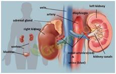
To get rid of substantial inter-observer inconsistency in kidney CTScans interpretation, Machine Learning (ML) provides a compact and objective basis for analytic calibration to notify clinical decisions. Current advances in imaging segmentation, registration, and classification through Deep Learning (DL) have significantly expanded the opportunity and scale of imaging analysis [7]. DL adapted to diagnostic applications may diminish unnecessary and offensive procedures, there- fore greatly refining the sustainability and efficiency of current healthcare schemes. Furthermore, with the extraordinary increase in computer science performance and real-time computer assisted diagnosis may additionally change telemedicine and mobile telecare. In the existing Kidney Carcinoma care prototypical, it relics controversial kidney role should be regularly partitioned in all symptom-less adults. The utmost commonly utilized Kidney Carcinoma screening assessments comprise testing the urine and blood for protein or serum creatinine; though, there is no decisive evidence signifying which screening trial is more suitable to the further in the situation of routine screening. Evolving an easily obtainable and non-invasive image indicator of kidney role using deep learning methods therefore may deliver a valuable courtesy tool for identifying Kidney Carcinoma. To discover this opportunity in clinical preparation, we established a deep learning algorithm which is based on kidney CTScanss imaging and medical data in a bulk registry-based Kidney Carcinoma cohort Figure 1.

2.1. Deep Learning in Medical Imaging

In healthcare, particularly in haematology, which is essentially cancer-related. One of the cancer challenges is that a lot of cancers are curable and diagnosed early on today. In order to detect whether there is cancer or not, an image was taken of a patient. You need

a doctor in order to diagnose cancer. As the number of experts is also reduced. So, if we use deep learning, artificial intelligence or automation here, then the machine will decide if a specific patient has cancer or not with a certain amount of precision. The detection process could be quicker than the specialist [11, 12] to manipulate the prediction or detection process of a disease such as cancer.

2.2. Motivation for selecting Deep Learning

In more than 3000 Kidney diseases affect 2 in every 3 people. It is very difficult to diagnose. 50 percent of the diagnoses in a public hospital is incorrect. The Kidney problem is extremely costly because of unnecessary visits, tests and treatments to general practitioners because of incorrect diagnoses. Most people have also no access to a Hematologists. So, Machine Learning and Artificial Intelligence can be used to support image classification using Deep Neural Networks (DNN). When an image, data, or information of Kidney is input to a machine it recognizes the morphology of the Kidney disease and produces some kind of different diagnosis as the earlier prediction. To provide decision support this can be faster and better than the other traditional methods. ML and Deep Learning improve the knowledge and skills in primary care and substitutional detection in cost.

As there are two kinds of Kidney Tumors, malignant Tumor Detection and non-malignant. Malignant Tumor has a dangerous implication because it can extend and damage other portions of the body parts. In the case of the deadliest diseases like Tumor, detection in early stages play a vital role in finding the probability of getting cured. At the primary stage, it is a challenge for a medical practitioner to differentiate a common Kidney tumor from modest benign tumors.

Kidney cancer has impacted many people’s lives and the diagnosis of kidney cancer plays an important role in assessing the likelihood of survival in the early stages. To promote early detection and affordably warn people who may be at risk, we can use advanced Deep Learning techniques. This instrument is not always precise and is not meant to be a substitute for clinical treatment. The core contributions of this research are as described below:

a. In order to produce a high quality and balanced image, certain pre-processing techniques are carried out with test sets built only from images of tumors.

b. For noise removal, we adapted the morphological filtering to

Figure 1: Body Structure of Kidney

shrink image regions and Conversion into Grey-scale as it is difficult to operate an RGB image. We perform a filtering process named Black Hat, as it converts an image including the objects of the input image. We applied thresholding on images as it is a segmentation process. This is done to separate object pixels from background pixels. After that, we reconstruct our missing part of images using image Inpainting.

1. To balance the imbalanced data, we have used augmentation techniques to increase the training dataset.

2. We used Modified CNN model for the classification of our model.

3. Related Works

The existing techniques used for Kidney Cancer detection and classification are efficient but need some improvements for the sake of accuracy. Most of the work done can classify Kidney tumors, however, limited work is done on the classification of multiple diseases. In recent researches, various techniques have been introduced by the researchers to diagnose and differentiate Tumor Detection from other Cancers. suggested two methods for the neural network, a back- propagation method, a radial-based purpose and a non- linear Support Vector Machine classifier. (SVM) and, in agreement with their performance and precision, equated. To achieve the best procedure with the above 3 procedures for Kidney Stone Diagnosis prediction, they used the method for completion. The main goal of their work was to provide the best medical diagnostic system, such as kidney stone identification, to minimize the time of analysis and improve skills and accuracy.

A data pre-processing, transformation, and mining method was suggested in [9] to obtain information on the collaboration between several computed constraints and patient life. The two separate deep learning processes were used in the form of decision rules to obtain knowledge. For their medical significance, essential variables detected by data mining were inferred. In their study work, they launched a new concept, which was used and analyzed using data obtained at 4 dialysis sites. In their paper, the suggested approach proposed to minimize the cost and work of selecting patients for medical studies.

A new work using machine learning processes was proposed in [7], Support-vector machine and random- forest, respectively. These data sets with evolving kernels and kernel parameters were applied to training, categorizing, and assessing kidney stone disease. The results of both were compared with different kernels separately, and the proper boundary set was tuned. To build successful learning processes for predictions, the findings were well examined. It is determined that different outcomes with different kernel tasks were analyzed with the sport vector machine classification method.

Two layers are feed forward perceptron trained with back-propagation training procedure and Radial-based feature systems for study of kidney stone infection in [10] suggested learning vector-quantization. The performance of all three neural networks was focused on their accuracy, algorithm development time and data set size training. Finally, the creators determined from the findings that a multi-layer learning model trained with back propagation is the best approach for the diagnosis of kidney stones.

A new technique for the diagnosis of optic-nerve dis- ease was proposed in [6] through the study of electroretinographic form signs with the help of artificial neural networks (ANN). The performed method of Multilayer back propagation. The final results were graded as being solid and diseased. The verified results suggested that an efficient study could be provided by the predicted technique.

The Subsequent Edge Distance and Pixel Wise Grouping Networks (SBD-PCN) for spontaneous kidney segmentation image CTScans were proposed in [11]. First, the authors defined pretrained deep neural networks to categorize images from CTScans images for high- level images, then used these functions as inputs with a mid-distance regression network to learn kidney limitations, and finally categorize the standard boundary space maps into kidney pixels with a pixel arrangement network. In a final learning technique, the segmentation of the kidney image is built on deep CNNs to measure kidney and kidney edges.

The Adaptive Neuro-fuzzy Inference Method (ANFIS) suggested in [12] the prediction of chronic renal failure. Here, the number of fuzzy rules refers to the number of relationship functions of input variables. ANFIS neural networks were used to classify glomerular categorization rates and to correlate system accuracy. To guess very accurate GFR, modeling and prediction results from ANFIS networks display the models based on the fuzzy system. Significant alerts from physicians are the efficacy and frequent monitoring of RCC (Kidney Carcinoma) patients in minimizing disease development and preventing such difficulties. This research for final help in the field of kidney disease and kidney carcinoma management in a numerical way was a key method for raising its problem in the use of the successful prediction model.

The Pattern Discovery Algorithm based on the mentioned revised joint material (PDA-ADMI) in chronic kidney failure was suggested in [13]. A reviewed version of popular knowledge is given in this paper to distinguish the negative and positive relationships. The writers revealed 16 real patterns that were physically examined by a medical doctor about the disorder. They proved that by popular details and incorporated n-class recommendation doctrines into the PDA-ADMI model, the group is super additive to decrease the calculation complexity. Using data conditions, algorithm analysis was carried out and medically assembled to consist of 16 patterns.

The Pathological Approximate Fibrosis Score (PEFS) on deep learning for the identification of chronic renal syndrome was suggested in [14]. A deep learning approach was applied to combine patient-specific histological entities with scientific phenotypes, such as serum creatinine, biopsy nephrotic proteinuria, kidney carcinoma, 1 to 3 and 5 years’ renal survival. The suggested CNN models surpassed PEFS by classification jobs and predict the point for the Kidney Carcinoma more precisely than the system PEFS. [15] proposed an assessment of chronic kidney diseases by the Support Vector Machine and Artificial Neural Network (SVM- ANN). All misplaced data values have been substituted for experimentation by means of the corresponding characteristics. Subsequently, SVM aims to provide the optimum parameters and ANN relies on numerical analysis. In addition, ANN and SVM were recognized by the Enhanced parameters.

Their research arrangements with the ’HMANN’ methodology, which has been suggested for the identification of kidney stone procedure, to get rid of various problems as argued in the overhead survey. In addition, the highest accuracy is demonstrated by ANN and wavelets for clinical organizational outcomes. In addition, if data and time are insufficient, the diagnostic syndrome can be helpful if incomplete diseases are identified and detected [16]. This paper uses ANN to deliver an excellent technique for a minimal diagnosis.

4. Dataset Collection

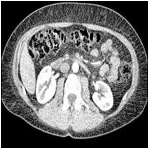
We have used KiTS19 (Kidney Tumor Segmentation Dataset 2019) openly available on Kaggle, to achieve segmentation and classification of tumors. This set contains upto 1000 images. We will be creating high quality,A balanced dataset of test and validation sets constructed solely from tumor images with one associated image. This is critical because if our model learns from an image of a given tumor, our accuracy would be unrealistically exaggerated if it is checked on another image of the same tumor. A sample image taken from the dataset is shown in Figure 2.

5. Proposed Methodology

This section explains the working flow of the proposed method using Deep Learning techniques.

5.1. Overview

On the (KITS19) dataset, we want to perform a 3- fold cross-validation for kidney tumor segmentation. To accomplish this, we are using our medical image segmentation techniques with with Convolutional Neural Networks and Deep Learning.

The goal of this study is to provide a quick construction of pipelines for medical image segmentation, including data input/output, preprocessing, data augmentation, patch-wise analysis, metrics, a library of state-of-the- art deep learning models and model utilization such as training, prediction and fully automated evaluation (e.g. cross-validation). With Tensor flow as the backend, our approach is based on Keras.

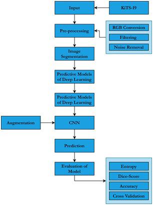
We have selected 300 kidney cancer patients CT scans images from dataset. One of three groups had to be named for each pixel: history, kidney or tumor. The image resolution of the initial scans is 512x512 and an average of 216 slices (highest slice number is 1059). A block diagram of our purposed methodology is shown in Figure 3.

3: Proposed Methodology

5.2. Pre-processing of Dataset

Kidney images are mostly exposed to noise mainly due to bad light, noise and air bubbles. It includes noise removal, resizing of image and shading removal. These steps provide a way for further steps. We find useful information from the pre-processing of metadata. Exploratory data analysis is also lying in this section. Medical images are most prone to noise such as Gaussian noise.

Figure 2: Sample Image taken from Dataset

Figure

In general, preprocessing techniques can handle the noise of the images and deep learning techniques learn to avoid these noises while making classification and predictions, though their ability to learn is conditioned upon the availability of large training data. In the case of medical Kidney images datasets, which are mostly imbalanced datasets, the Deep Learning models are easily susceptible to overfitting, i.e. they utilize visual hints such as noise indicators of the cancer category.

The first step in the pipeline is to establish a Data I/O. It offers the utilization of custom Data I/O interfaces for fast integration of your specific data structure into the pipeline.

We have used data preprocessing techniques to remove noise and noises on the images. We have modified the noise removal algorithm. The steps include:

5.2.1. Conversion into Gray-scale: The arrangement of sharpness, shadow, contrasts and construction of the color picture are novel procedures. To alter the Red Green Blue (RGB) into grayscale, an average method is used.

5.2.2. Conversion into the Black-Hat: The black hat is an image filtering process. We have used this filtering for the following reason. It proceeds an image that contains the basics of the input image that are lesser than the configuring component and dimmer than their surroundings.

5.2.3. Morphological Filtering: We have used the structuring element as a morphological operator. It affects the regions of images. We apply this filtering for eliminating the unnecessary regions in the images on the pixels of the image. Following is the basic flow of morphological filtering shown in Figure 4. The crosses shown in Figure. Similar to the origin of the structuring feature, 4. It is very important to locate this place of origin. When we pass it over the image pixels, it sets the window’s reference location, and thus the structuring element.

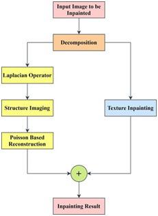
image, the exemplar-based method is then used. Afterwards, via the Poisson equation, we reconstruct the structure image from the restored Laplacian image and thus obtain the repaired outcome of the structure image. Finally, to achieve the painting output of the original image, these two sub-images are added back together. By this means, both structure and texture information is well restored.

Figure 4: Morphological Operations

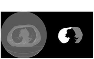
5.2.4. Binary Thresholding: It is a modest procedure of image segmentation. It is a technique to produce a binary image from an RGB image or grayscale. Typically, we use this to separate foreground pixels from the background pixels.

5.2.5. Inpaint Telea: In Inpaint methodology, we split the image into two components: the images of the structure and texture, and then separately restore the two components according to their image characteristics. Using the exemplar-based process, the texture image is repaired, since the method is derived from the techniques of texture synthesis. Fig. Figure 5 As for the structure image, the Laplacian operator is applied first to boost the structure knowledge and to obtain the Laplacian image. To repair the Laplacian

5.3. Pre-processed Data

As to validate our model properly, we have pre- processing steps. We create high quality, the balanced dataset for testing and validation as our downloaded dataset was unbalanced. We used to remove noise in pre-processing that was mainly due to bad light, noise and air bubbles. These steps (conversion into grey-scale, morphological filtering, conversion into a Black hat, applies threshold, Inpaint) provide us clear enhancement to further steps. The preprocessed results are shown in Figure 6.

6: Preprocessed Data

5.4. Augmentation

To improve the learning capability of the model and to generalize its performance, image data augmentation is used. Augmentation is a technique that is used by making updated copies of images in the dataset to artificially increase the size of a training dataset. After the Data I/O Interface initialization, the Data Augmentation class can be configured.

A Preprocessor object with default parameters automatically initialize a Data Augmentation class with default values, but here we initialize it by hand to illustrate the exact workflow of the meth-

Figure 5: Framework for Inpainting technique

Figure

odology.

The parameters for the Data Augmentation configure which augmentation techniques should be applied to the data set. In this case, we are using all possible augmentation techniques in order to run extensive data augmentation and avoid overfitting.

5.4.1. Selective Data Augmentation: Noticing that our dataset is still imbalanced, for our training set, we selectively augmented each class. For each image in a given class, we used Keras Image Data Generator to generate several augmented images. We produced more augmented images for the classes with less images to end up with a training set where all classes are relatively portrayed equally.

5.4.2. Augmentation Multiplier: If there were 4000 images in our largest class and 200 images in our smallest class, our augmentation multiplier for the smallest class will be 20. We will thus produce 20 augmented images for each image in the smallest class. The largest and smallest classes would then be balanced if we left our largest class alone. For our real dataset, below is an implementation of this theory. First, for every class name and its related index, we construct a data frame and then we describe our ’augmultiplier’ in terms of the size of our largest class.

5.4.3. Generate Augmented Data: Note that at this stage, we are not normalizing our data because when we load up our data for model training, we will normalize based on Image-Net stats. It was possible to change the hyper parameters for this Image Data Generator, we selected these parameters to generate ample variety while preserving the overall structure. For now, our dataset contains only the augmented images shown in figure 7 that we have just created. With these augmented images, we will then add the original images.

5.4.4. Append Original Images: When we use the Keras Image

Figure 7: Modified CNN Architecture Data Generator, several slightly changed versions of our original images are loaded. Our training archive, therefore, contains none of our original photos. We will now append the original photos into the training folder to complete our dataset. In addition, we will add the photos that have been set aside to their relevant folders for testing and validation. Our complete dataset after augmentation is shown in Figure 11.

5.4.5. Augmented Data: After the process of artificial expanding of the data set, an augmented dataset is received that dataset ready to use for learning in our model. This data improves our model performance as mention above in the augmentation section.

5.5. Model Building

5.5.1. Classify Kidney Images: In our build model section, we have introduced Fastai methodologies. In the Fastai method, the first step is to initiate the CNN Model. Then we train the model on our training data and find the optimal learning rate.

5.5.2. Introduce Fastai Methodologies: Since the API is designed on top of the lightweight PyTorch, we decided to use fastai and natively supports some nice approaches that are not easily implemented in other frameworks. Below, some of the basic advantages we get from these strategies are covered and a description of why they benefit. The modified Model of CNN is shown in Figure 7.

5.5.3. Wd: As an alternative to L2 regularization, this weight decay concept was added. As with other techniques of regularization, this concept is used to decrease network weights over time, eliminating over-fitting.

5.5.4. Lr. Find: As the most important hyper-parameter for training a neural network, the learning rate is generally accepted. This technique goes through a trial run, beginning with a low learning rate and growing it with each batch exponentially. From the loss vs. learning rate map, we can choose the highest learning rate where our loss is still falling dramatically.

5.5.5. Fit-One-Cycle: In our approach to setting the learning pace, this extremely effective technique emerged in [47] and is another leap forward. In short, this approach works by sweeping through a variety of learning rates and helps the model to converge faster and find better local minima (by not getting stuck in the first valley it comes to).

5.5.6. Max-warp: This is a hyper-parameter of image transformation provided in a few augmentation libraries. Warp simulates tilting the view that the image was taken from. In our case, this is particularly true because most of the images in our dataset are taken from directly above the tumor of the kidney. Our model may not be prepared to identify the tumor if we checked this model on a new picture and took it from a more oblique angle. Our model becomes more stable for new data by applying warp to our dataset.

5.6. Instantiate CNN model

CNN is low-power, low-latency and small models parameterized to fulfill the resource limits of a type of use case. Figure 8 shows the CNN architecture. CNN can be used for recognition, segmentation, embedding’s and classification similar to how other famous models, like Inception, are used. CNN recovers the state-of-theart performance of mobile models on numerous tasks and targets as well as across a spectrum of dissimilar model sizes. CNN can be run efficiently on mobile devices with TensorFlow Lite. The

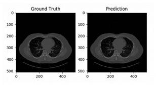
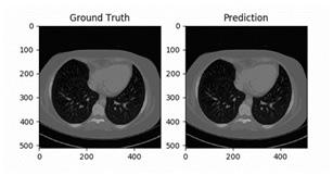
Figure 11: Ground Truth and Prediction of Case 44 with Slice 0

processing of this section is shown in Figure 8.

5.7. Training Model for Classification of Tumor

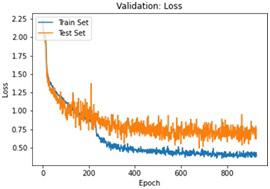
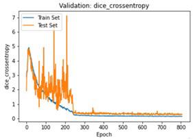
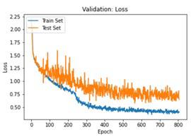
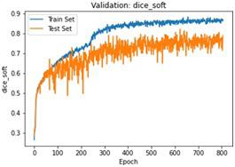
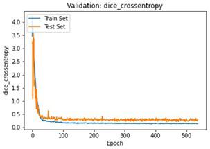
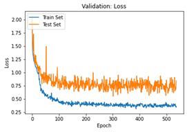
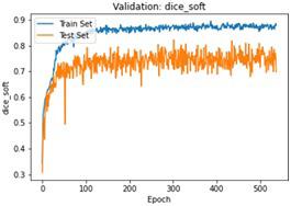
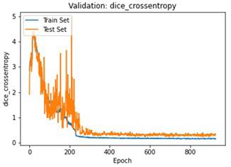
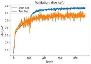
We have to train our model to find the optimal learning rate. Set our learning rate to the value where learning is fastest, and loss is still decreasing. We developed a function that uses our input as an anchor and sweeps through a range to search out the best local minima. The model validation loss and cross entropy with dice scores of three folds are shown in (Figure 14-22). We can see that losses decrease exponentially as the validation of the number.

Figure 8: Processing of CNN

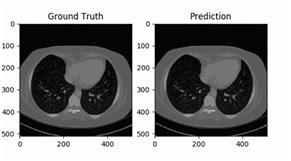
Figure 12: Ground Truth and Prediction of Case 18 with Slice 0

Figure 13: Ground Truth and Prediction of Case 38 with Slice 0

Figure 14: Validation Score of our model CV-1

Figure 15: Validation Loss of Our Model CV-1

Figure 16: Validation Cross-entropy of Our Model CV-1

Figure 17: Validation Score of our model CV-2

Figure 18: Validation Loss of Our Model CV-2

Figure 19: Validation Cross-entropy of Our Model CV-2

Figure 20: Validation Score of our model CV-3

6. Experimental Evaluation

6.1. Tumor Segmentation

2D image segmentation, results for each case were analyzed in three dimensions, with specific criteria for inclusion and exclusion in the final volumetric segmentation. Kidney regions with tumors of different types were validated depending upon conditions of volume and position. The ground truth and prediction of our build model is shown in Figure 9.

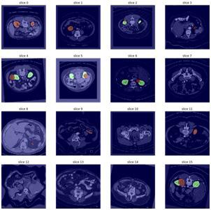
our model to detect. Figure 9 shows some of the random samples that were difficult for our model to detect. At every sub-image and some parameters are shown. These parameters are: • Prediction: tumor predicted by the model • Actual: Actual tumor that the model could not predict. • Loss: Losses occur during predicting the random image. • Probability: Probability of the model to predict the tumor correctly.

Prediction of the ground truth of different cases with slice 0 is shown in (Figure 10, 11).

Let’s take a look at some of the samples that were most difficult for

The model predicted it as Malignant Tumor Detection, however it was Benign. The losses occur during the prediction of this random image 0.01 and the probability to predict this random sample was 0.

6.2. Performance of Model

We provided some random images one by one to the model. Since our main focus was to detect Kidney tumors. The ‘prediction interval’ guesses in which value a future individual reflection will fall, whereas a ‘confidence interval’ displays the likely value of ranges related to the statistical constraint of the information, i.e., the mean of the population.

Our model does not only detect Tumor Detection, but it can also detect other Kidney tumors with an impressive less loss. Figures below shows the performance of our model.

In the figures above it can easily be seen that Validation Loss in all of the folds is decreasing eventually with respect to time.

7. Conclusion

In this research work, we had an image of a CT- Scan of a kidney containing a tumor. We applied the Morphological Filtering for the Image Enhancement followed by Histogram Equalization. The restored image went under Image Segmentation, namely, Watersheds after which Marking was done and the final image was produced. The final image showed a distinct location of the stone in the kidney. Hence the stone was detected. We used the CNN

Figure 21: Validation Loss of Our Model CV-3

Figure 22: Validation Cross-entropy of Our Model CV-3

Figure 9: Segmentation and Detection of Tumor after 3 folds of Cross Validation

Figure 10: Ground Truth and Prediction of Case 24 with Slice 0. x

Figure 11: Ground Truth and Prediction of Case 44 with Slice 0

model for testing our sets. We train the model on our training data and found the learning rate of the model. Then we estimate the confusion matrix and accuracy of the trained model. Accuracy of our trained model range from 90-99 percent and are considered as the best accuracies. The model predicted the Tumor Detection with confidence level ranges from 70-100 percent depending on the resolution of the image. The model also successfully predicted and classify other Kidney tumors with a very high confidence. For future work, one can suggest the implementation of this automated method for the detection of Kidney tumors into smartphones/Tabs. We can also optimize the learning rate of the classifiers.

Kidney images can be sliced into layers so that more accurate detection may perform at higher accuracy.

References

1. Ma F, Sun T, Liu L, Jing H. Detection and diagnosis of chronic kidney disease using deep learning-based heterogeneous modified artificial neural network. Futur. Gener. Comput. Syst. 2020; 111; 17-26.

2. Wibawa HA, Malik I, Bahtiar N. Evaluation of Kernel-Based Extreme Learning Machine Performance for Prediction of Chronic Kidney Disease. in 2018 2nd International Conference on Informatics and Computational Sciences, ICICoS. 2018; 2019: 33-6.

3. Rady EHA, Anwar AS. Prediction of kidney disease stages using data mining algorithms. Informatics in Medicine Unlocked. 2019; 15: 100178.

4. Gharibdousti MS, Azimi K, Hathikal S, Won DH. Prediction of Chronic Kidney Disease using data mining techniques. 67th Annu. Conf. Expo Inst. Ind. Eng. 2017; 2135-40.

5. Revathy S, Bharathi B, Jeyanthi P, Ramesh M. Chronic kidney disease prediction using machine learning models. Int. J. Eng. Adv. Technol. 2019; 9(1): 6364-7.

6. Vijayarani S, Dhayanand S. Kidney Disease Prediction Using Svm and Ann Algorithms. Int. J. Comput. Bus. Res. 2015; 6(2): 2229–6166.

7. Sinha P, Sinha P. Comparative Study of Chronic Kidney Disease Prediction using KNN and SVM. Int. J. Eng. Res. 2015; 4(12): 60812.

8. AhmedK A, Aljahdali S, Hussain SN. Comparative Prediction Performance with Support Vector Machine and Random Forest Classification Techniques. Int. J. Comput. Appl. 2013; 69(11): 12-6.

9. Abhishek, et al. Proposing Efficient Neural Network Training Model for Kidney Stone Diagnosis. Int. J. Comput. Sci. Inf. Technol. 2012; 3(11): 3900-4.

10. Kumar K, Abhishek A. Artificial Neural Networks for Diagnosis of Kidney Stones Disease. Int. J. Inf. Technol. Comput. Sci. 2012; 4(7): 20-5.

11. Yin S, et al. Automatic kidney segmentation in CTScans images using subsequent boundary distance regression and pixelwise classification networks. arXiv. 2018.

12. Norouzi J, Yadollahpour A, Mirbagheri SA, Mazdeh MM, Hosseini SA. Predicting Renal Failure Progression in Chronic Kidney Disease Using Integrated Intelligent Fuzzy Expert System. Comput. Math. Methods Med. 2016; 2016: 6080814.

13. Perkovic V, et al. Canagliflozin and Renal Outcomes in Type 2 Diabetes and Nephropathy. N. Engl. J. Med. 2019; 380(24): 2295-306.

14. Kolachalama VB, et al. Association of Pathological Fibrosis With Renal Survival Using Deep Neural Networks. Kidney Int. Reports. 2018; 3(2): 464-75.

15. Almansour NA, et al. Neural network and support vector machine for the prediction of chronic kidney disease: A comparative study. Comput. Biol. Med. 2019; 109: 101-1.

16. Alelign T, Petros B. Kidney Stone Disease: An Update on Current Concepts. Advances in Urology. 2018; 2018: 3068365.