,
\’
\
Y.,
‘$
\ ‘,
‘,\ “y
\ ‘,
‘“
\ t \
\ “\
“t . .
;$ \
\’\,
t
‘
+
I
\
“,
~,\ J..},
. .)
’”,
-.’!
-.
‘“,, \
.\
‘,,
“t\
‘$ ~
%,
“1 \’ ,, 4 CKY ,
‘$,’\~
“\.:’\ ‘,
‘..\
\“, !300
~L “.
‘““
“)
,,{
\ , >–x
\ -, \
-.
‘\ 4> ??
‘“
w“:
!~ \ %e
‘$,R \
:’\
~ ‘!
\\\ ‘\
i- 300
A ;.
‘\
\
‘,
‘ \“%
!
\ \,\\
-x..
~ “,
y“, ‘, ISOBARS
,
(rob)
,
‘. \
—
- -,, :1
rod;
+.’OO -40”
- 3V
-20”
‘~i’-\
-1o”
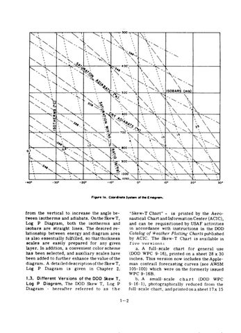
FIIAWO10.
bdmto
Sptan
Different
P
Diagram
Versions
\
! .-
~.\i ‘?. 10”
\
\l
,
+k+r 20”
\ \
>,\
—
30”
of ttn ErmgrmL
“Skew-T Chart” - is printed by the Aeronautical Chart and Information Center (ACIC), and can be requisitioned by USAF activities in accordance with instructions in the DOD Catalog of Weathev Plotting Charts published by ACIC. The Skew-T Chart is available in five versions: a. A full- scale chart for general use (DOD WPC 9- 16), printed on a sheet 28 x 30 inches. This version now includes the Appleman contrail forecasting curves (see AWSM 105- 100) which were on the formerly issued WPC 9- 16B. chart (DOD WPC b. A small-scale 9-16- 1), photographically reduced from the full-scale chart, andprinteci ona sheet 17x 15
has been selected, and auxiliary scales have been added to further enhance the value of the diagram. A detailed description of the Skew T, Log P Diagram is given in Chapter 2.
Log
I \
o“
from the vertical to increase the angle between isotherms and adiabats. On the Skew T, Log P Diagram, both the isotherms and isobars are straight lines. The desired relationship between energy and diagram area is also essentially fulfilled, so that thickness scales are easily prepared for any given layer. In addition, a convenient color scheme
1.3.
,;,
of the DOD Skew T,
The DOD Skew T, Log P - hereafter referred to as t he
Diagram.
1–2