Figure Figure 6 represents the current readings of Zone 4 under normal conditions where x-axis represents the time of simulation and y- axis represents the current readings of the line (in Amperes) under normal conditions. Steady state is reached at around 190A at a simulation time of 0.4 seconds.

Figure 7

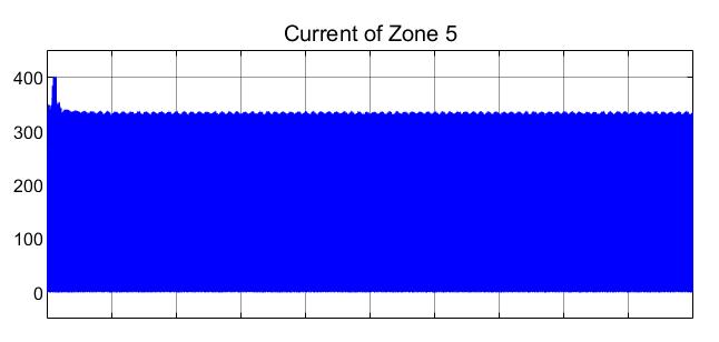
The current readings under normal conditions (in Amperes) of Zone 5 is presented in Figure 7. There is a momentary spike of 400A which is observed for a few cycles, after which a steady state value in transients between 0A and 310A is observed.

Figure 8

Figure 8 represents the current through Zone 6 under simulation of normal conditions, i.e. where no fault or disturbance affects the system under consideration. There is an initial spike observed to about 3000A after which the current reduces drastically. This is followed by a reach to steady state value by the current readings at around 100A.

Figure 9

The current readings of Zone 7 (in Amperes) under normal conditions is Figure 9, where x-axis represents the time of simulation and y-axis represents the current readings of the measurement unit in Zone 7. An initial drop to almost -500 A is observed for a few cycles after which the value stabilizes to transients between 0A and about 400A, thus reaching steady state by around a simulation time of 0.07A.

Figure 10

Figure 10 displays the current readings, in Amperes, in Zone 8 under normal conditions. The value of current drops to -2.6×10^(-4) A and reaches a steady state value of -2.5×10^(-4) A at a simulation time of around 0.05 seconds.

Figure 11

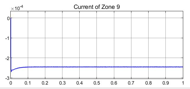
The current of Zone 9 under normal conditions, where x-axis represents time of simulation in Simulink and y-axis represents the current reading in A, is displayed in Figure 11. The value of current drops to -2.6×10^(-4) A and reaches a steady state value of 2.5×10^(-4) A at a simulation time of around 0.05 seconds.

B. Simulation Results and Analysis – Under Pole to pole fault condition

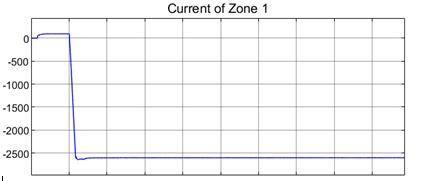
Figure 12

When a pole-to-pole fault is simulated at Zone 1, the current change is observed and displayed in Figure 21. While the x-axis represents the simulation time in seconds, y-axis represents the current of Zone 1 in Amperes. The fault is created in about 1.000 second of simulation time and it is observed that the current drops from a steady state value of around 95A to a value of around 2600A and stabilizes there.

Figure 13

When a pole-to-pole fault is created at Zone 1, Figure 13 showing the current measurements of Zone 2 shows that there is a decrease in current from around transients between 0A and 320A to transients between 0A and 280A.

Figure 14

Figure 14 shows the current observations in Zone 3 when a p-p fault is created in Zone 1. When a fault is created, the value of current shows a drastic, immediate increase from a steady state value of 100A to 1900A. This value decreases to around 1600A and stabilizes with transients.

Figure 15

When a p-p fault is created a Zone 1, Figure 15 displays the current measurements in Zone 4, when the fault is created at a simulation time of 1.00. When the fault is created, a momentary decrease to -5500A from steady state value is observed followed by stabilization with transients around -2500A.

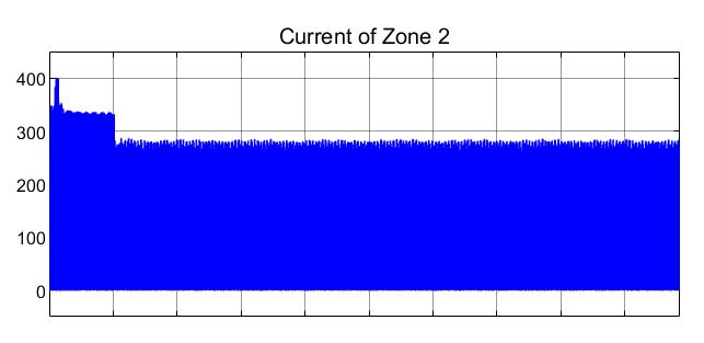
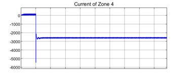
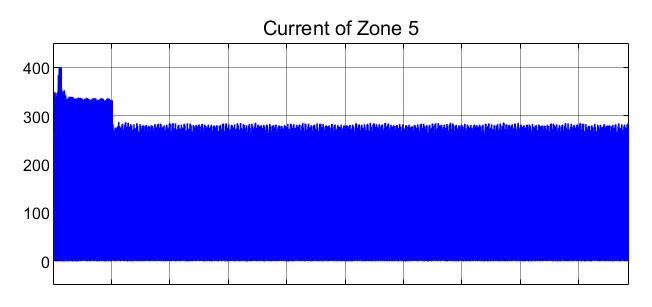
Figure 16

When a p-p fault is created at Zone 1, Figure 16 shows Zone 5’s current measurement with x-axis representing the simulation time and y-axis representing the output of the current measurement device. Once the fault has occurred, decrease in the observed transients from 0A to 325A to stabilization between 0A to 280A is observed.

Figure 17

Figure 17 shows the measurement of current at Zone 6 when a p-p fault occurs at Zone 1. When the fault has occurred at a simulation time of 1.000, a sudden spike in current is observed followed by a stabilization with transients around 1600A.

Figure 18 Figure 18 represents the current through Zone 7 when a p-p fault is created at Zone 1 at a simulation time of 1.000. The observed current shows a decrease to -1450A from steady state value and a slight increase to stabilization at -1100A.

Figure 19

Figure 19 represents the current through Zone 8 when a p-p fault is created at Zone 1 with x-axis representing the time and the yaxis representing the current of the Zone in Amperes. The current value increases from steady state value to a peak at -1x10^-4A to stabilization with transients around -1.15x10^-4A

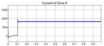
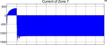
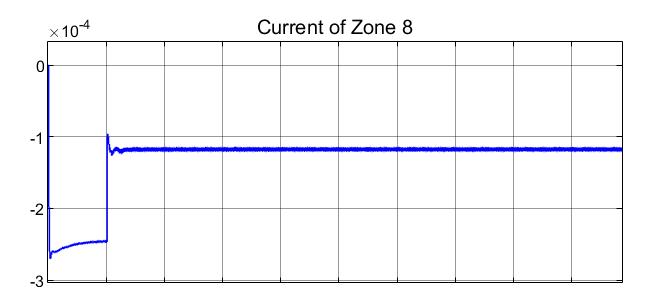
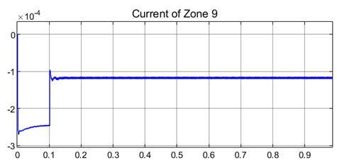
Figure 20

Figure 20 represents the current measurement in Zone 9 after a fault has been created at a simulation time of 1.000 in Zone 1. The current value increases from steady state value to a peak at -1x10^-4A to stabilization with transients around -1.15x10^-4A.

C. Comparative Analysis of PP and PG Faults at Zone 1 in the selected microgrid

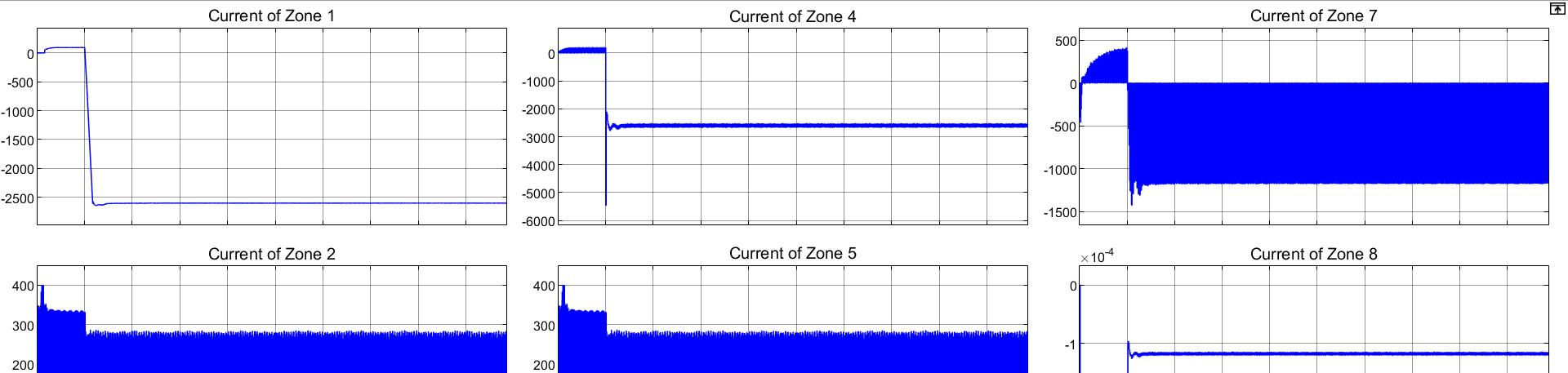
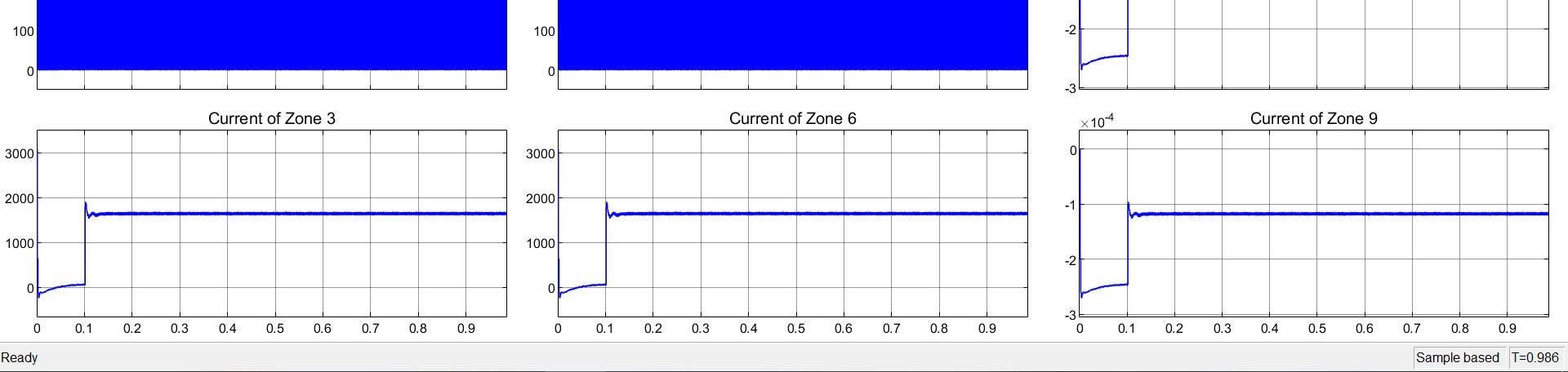
Figure 21

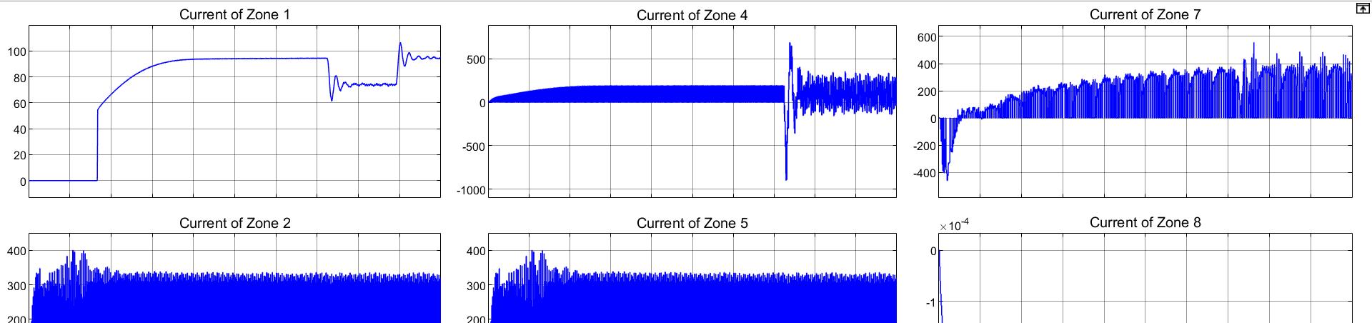
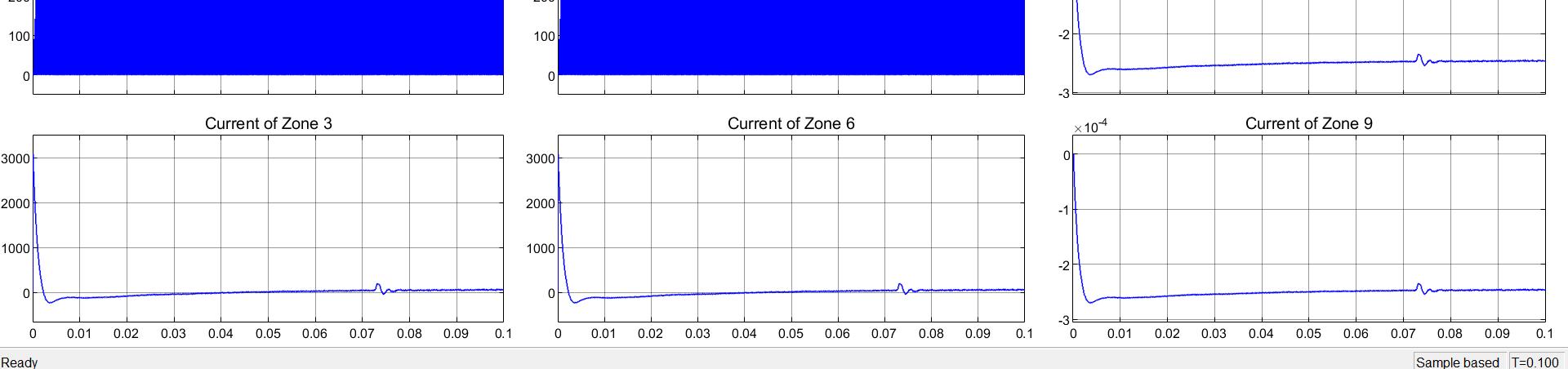
Figure 22

When a pole-to-pole fault is created at Zone 1 as shown in figure 21, the current of zone decreases from a steady state value of approximately 95A to a value of approximately -2600A. The pole-to-pole fault is simulated at a simulation time of 1.00 seconds. However, when a pole to ground fault is created at zone one at a simulation time of 0.07 seconds, Current of all the zones are shown at once (each one explained in earlier section) and the current of zone 1 shows a decrease from the steady value of 95A to around 75A. This decrease is occupied with high harmonics and transients. About 0.02 seconds later, the current increases to the previous steady state value, maintaining the high number of transients. From Figure 22, It is concluded that a pole-to-pole fault in the studied system has a more severe effect on current than a pole-toground fault on the same system. For protecting the system considered against various types of faults, current change has been monitored at various places with the help of measuring devices available in the mat lab tool box.Fourier transform method has been applied to locate the fault.

D. Algorithm Applied: In this section of the paper current algorithm for the controller has been discussed which is applied to the microgrid under consideration. Current algorithm works on the principle of finding deviation of the current of the zone with the current of the same section ‘n’ samples ago. In this case value of number of samples taken is 200 per second. From the current waveforms of various zones shown above, when a fault is created there is a sudden change in the current off that zone and 200 samples back current value has been taken to find the sufficient change in the current of the same zone. Change in current of a particular zone ( ΔI ) = Present value of the current - current value 200 samples ago. Following is the algorithm used for fault detection location

ΔI= Ip-Is (200 samples back))

Current algorithm for fault detection and location for the system under consideration

Start

Measure I Calculate the value of I 200 previous samples ago Delta = I – Iprev If delta >= 0.1*Iprev Fault detected F=1 Else Fault not detected If F=1 Start fourier transform of current values Calculate runningmax of magnitude of fourier transform Runningmax[7] is obtained Calculate max of all runningmax If max == runningmax[0] Fault at 1 If max == runningmax[1] Fault at 2 If max == runningmax[2] Fault at 3 If max == runningmax[3] Fault at 4 If max == runningmax[4] Fault at 5 If max == runningmax[5] Fault at 6 If max == runningmax[6] Fault at 7 Repeat until simulation is stopped

Fault is created at 0.051 seconds in zone 4 – breaker of zone 4 shows OFF state Using current algorithm

Figure 23

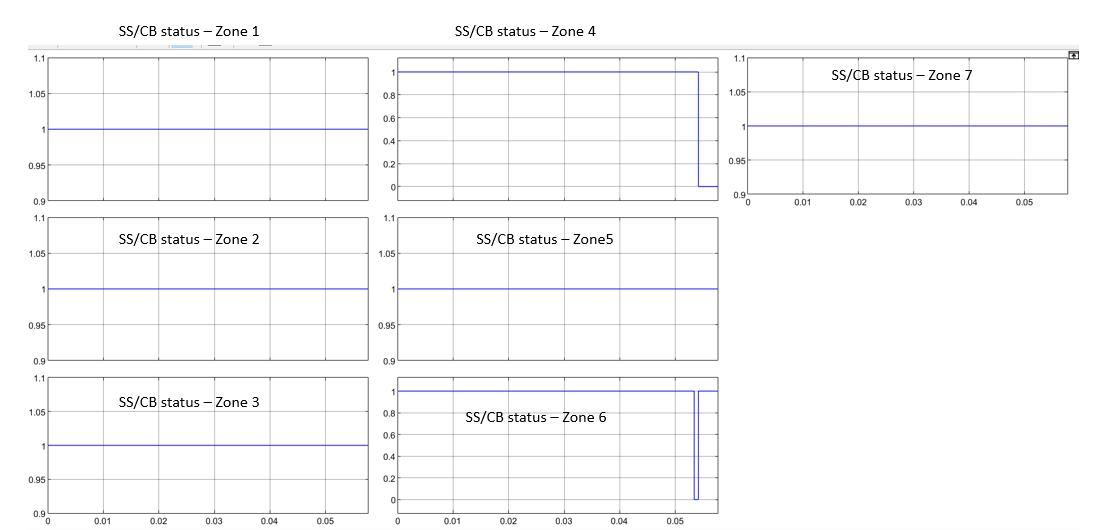
When fault is created at 0.052 seconds the breaker of zone 4 shows OFF state in figure 23 . Fault in 6th zone was also sensed for very short duration, though it did not operate the circuit breaker / smart switch whereas all other CB’s or smart switches are closed and showing status as 1. Current algorithm has been applied to the system under consideration, this algorithm is a memory-based algorithm which required 0.052 seconds wait time to reach steady state before disturbances or faults can affect the system. This algorithm was successful in detecting pole to pole faults and pole to ground faults in the system under consideration. This Current change algorithm made use of dynamically updated values for the operation of smart switches (Isolation switches). It was observed that this method is unable to identify the location of a fault. It takes more than 1 hour to simulate for 0.5 seconds. It took wait time of 0.05 seconds (prerequisite) for the system to reach steady state. So, it is not strongly advised to apply this algorithm for rapidly changing load conditions and irradiation

IV.CONCLUSIONS

Fault Analysis for the system under consideration has been carried out. Current change algorithms has been applied with in the controller for the detection of fault in the microgrid, whereas Fourier transform method has been applied for locating the fault in the microgrid. Current change algorithm is a memory-based algorithm which required some wait time 0.052 seconds wait time to reach steady state before disturbances or faults can affect the system. This algorithm was successful in detecting pole to pole faults and pole to ground faults in the system under consideration. This Current change algorithm made use of dynamically updated values for the operation of smart switches (Isolation switches). It was observed that this method is unable to identify the location of a fault. It takes more than 1 hour to simulate for 0.5 seconds. It took wait time of 0.05 seconds (prerequisite) for the system to reach steady state. So, it is not strongly advised to apply this algorithm for rapidly changing load conditions and irradiation. Machine Learning Based Algorithm can be applied for the protection of microgrid in future as microgrids condition changes at a rate of sub milliseconds.

REFERENCES

[1] Magdi S.Mahmoud,Mohamed Saif Ur Rahman,Fouad M.A.L.-Sunni, “Review of Microgrid architectures-a system of systems perspective”, The Institution of

Engineering and Technology(IET) journal,29th April 2015. [2] Robert. H. Lasseter, Paolo Paigi, “Microgrid: A Conceptual Solution” 30th annual IEEE Power Electronics Specialists Conference, Germany, 2004. [3] Rahul Anand Kaushik, and N. M. Pindoriya, “A Hybrid AC-DC Microgrid: Opportunities & Key Issues in Implementation”, Electrical Engineering, IEEE. [4] Xiong Liu, Peng Wang and Poh Chiang Loh, “A Hybrid AC/DC Microgrid and Its Coordination Control”, IEEE transactions on smart grid, Vol. 2, No. 2,

June,2011 [5] Anoop Singh “A market for renewable energy credits in the Indian power sector”: Science Direct, Renewable and Sustainable Energy Reviews 13 (2009): 643–652 [6] Nanfang Yang, Damien Paire, Fei Gao, Abdellatif Miraoui, “Power Management Strategies for Microgrid -A Short Review”, IEEE,2013 [7] A Hybrid AC-DC Microgrid: Opportunities & Key Issues in Implementation Rahul Anand Kaushik, Student Member, IEEE and N. M. Pindoriya, Member,

IEEE Electrical Engineering, Indian Institute of Technology Gandhinagar Ahmedabad, Gujarat, India, Email: rahulanandkaushik@iitgn.ac.in [8] Fransic JavodaTHE KEY ROLE OF INTELLIGENT ELECTRONIC DEVICES (IED) IN ADVANCED DISTRIBUTION AUTOMATION (ADA)

Department of Electrical Apparatus, IREQ (Hydro-Quebec Research Institute), Varennes, PQ, Canada E-MAIL: zavoda.francisc@ireq. [9] JAFAR MOHAMMADI, (Student Member, IEEE), AND FIROUZ BADRKHANI AJAEI , (Member, IEEE)Electrical and Computer Engineering Department,

Western University, London, ON N6A 5B9, Canada” Adaptive Voltage-Based Load Shedding Scheme for the DC Microgrid” current version August 15, 2019 [10] Sangeeta Modi, P Usha “Mathematical modelling, Simulation and Analysis of Microgrid: A pre-requisite for Devising a Controller” GIS Science Journal, volume 8 , Issue 12 , December21 , ISSN No: 1869-9391