9 minute read
INFERENTIAL STATISTICS INTRODUCTION

Generalizability
Back again to the question poised at the introduction of this part, but now with some definitions. If we would like to study how many pupils have Type I Diabetes, then we will call the pupils our Target Population.
Advertisement
Again, do you think we have enough money and time to test every pupil’s blood glucose? of course not.
Therefore, we take a Sample. Now, it is much easier to test them and get a result that characterizes this sample, called a Sample Statistic. We then assume that what is true of the sample will also be true of the target population. Thereafter, based on the sample statistic, we make informed guesses, Inferences, to get conclusions about the whole population, expressed in an Interval Estimate.
This branch of statistics is called Inferential Statistics.
In simpler words, Interval Estimates are numbers that summarize data for an entire population. The Sample Statistics are numbers that summarize data from a sample, i.e. some subset of the entire population.
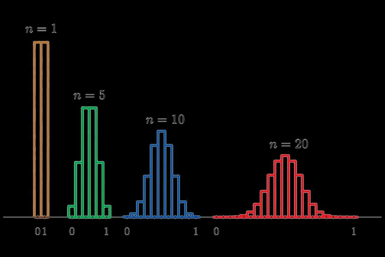
Central Limit Theorem Means Distribution

Typically, we collect data from a sample, and then we calculate the mean of that one sample. Now, imagine that we repeat the study many times on different samples and collect the same sample size for each one. Then, you calculate the mean for each of these samples and graph them on a histogram. That histogram will display the distribution of all samples’ means, which statisticians refer to as the sampling distribution of the means. (See Figure 1)
In the histogram, note that the more samples you study, the more your means’ distribution will look like a normal distribution (compare n=5 to n=20). This principle is called the Central Limit Theorem. The central limit theorem in statistics states that,
“Given a sufficiently large sample size, the sampling distribution of the mean for a variable will approximate a normal distribution regardless of that variable’s distribution in the population.”
Fortunately, we do not have to repeat studies many times to estimate the sampling distribution of the mean. Statistical procedures can help us estimate that from a single random sample. The take on this is that with a larger sample size, your sample mean is more likely to be close to the real population mean, making your estimate more precise.
Therefore, understanding the central limit theorem is crucial when it comes to trusting the validity of your results and assessing the precision of your estimates.
Normality Assumption
Part of the definition for the central limit theorem is “regardless of the variable’s distribution in the population.” This part is vital. In a population, the values of a variable can follow different probability distributions. These distributions can range from normal, left-skewed, rightskewed, and uniform, among others.
The central limit theorem applies to almost all types of probability distributions. The fact that sampling distributions can approximate a normal distribution has critical implications.
In statistics, the normality assumption is vital for parametric hypothesis tests of the mean, such as the t-test.
Consequently, you might think that these tests are not valid when the data are not normally distributed. However, if your sample size is large enough, the central limit theorem kicks in and produces sampling distributions that approximate a normal distribution, even if your data are not normally distributed.
Standard Errors
Striving for feasibility while conducting research forces you to pick a small sample from the whole population to get your measurements. Unfortunately for everyone but statisticians, almost certainly, the sample mean will vary from the actual population mean. This is when the Standard Error (SE) comes into play.
The magnitude of the standard error gives an index of the precision of the estimate of the interval. It is Inversely Proportional to the sample size, meaning that smaller samples tend to produce greater standard errors.
Confidence Intervals
The Confidence Interval (CI) is a range of values we are fairly sure our true value lies in. A 95% CI indicates that if we, for example, repeat our experiment a hundred times, we will find that the true mean will lie between the upper and the lower limits in ninety-five of them.
So how do we know if the sample we took is one of the "lucky" 95%? Unless we get to measure the whole population, we simply do not know. That is one of the risks of sampling.
Point Estimate vs Interval Estimate
Suppose a group of researchers is studying the levels of hemoglobin in anemic male patients.
The researchers take a random sample from the target population and establish a mean level of 11 gram/dl. The mean of 11 gram/dl is a Point Estimate of the population mean.
A point estimate by itself is of limited usefulness because it does not reveal the uncertainty associated with the estimate; you do not have a good sense of how far away this 11 gram/dl sample mean might be from the population mean.
Therefore, Confidence Intervals provide more information than Point Estimates. By establishing a confidence interval of 95% (= Mean ± 2SE), and binding the interval by the properties of the normal distribution through the bell curve, the researchers arrive at an upper and lower bounds containing the true mean at any time.
Confidence Intervals do not indicate how much of your datapoints are between the upper and lower bounds, but indicate how sure you are that your sample dataset reflects the true population.
Effect Size and Meta-Analyses
Expressing Differences
A usual scenario conducted in clinical trials on drugs is to give a group of patients the active drug (i.e. the real drug) and give the other group a placebo. The difference between the effect of the real drug and the effect of placebo is an example of the concept of Effect Size.
Effect Size is a statistical concept to quantify the difference between groups in different study conditions, therefore, quantifying the effectiveness of a particular intervention relative to some comparison. It allows us to move beyond the simple statistical significance of: “Does it work?” to “How well does it work in a range of contexts?”.
Expanding on the concept, the p-value can tell us that it is statistically significant that both ACE Inhibitors and β-Blockers can treat hypertension. However, it does not inform us which one is better; therefore, we use Effect Size.
Beyond the Results
One of the main advantages of using effect size is that when a particular experiment has been replicated, the different effect size estimates from each study can easily be combined to give an overall best estimate of the size of the effect.
This process of combining experimental results into a single effect size estimate is known as meta-analysis.
Meta-analyses, however, can do much more than simply producing an overall “average” effect size. If, for a particular intervention, some studies produced large effect sizes, and some others produced small effect sizes, would a meta-analysis simply combine them and say that the average effect was “medium” ? definitely not.
A much more useful approach would be to examine the primary studies for any differences between those with the large and the small effects, and then to try to understand what factors might account for the difference. The best effective meta-analysis, therefore, involves seeking relationships between effect sizes and characteristics of the intervention (e.g. context and study design).
Hypothesis Testing
Alternative Hypothesis & Null Hypothesis
Let’s say we have a group of 20 patients who have high blood pressures at the beginning of a study (time 1). They are divided into two groups of 10 patients each.
One group is given daily doses of an experimental drug meant to lower blood pressure (experimental group); the other group is given daily doses of a placebo (placebo group).
Then, blood pressure in all 20 patients is measured 2 weeks later (time 2).
A term that needs to be kicked into the game is the Null Hypothesis (H0). It is the statement that indicates that no relationship exists between two variables (in our example: the two groups).
Following statistical analysis, the null hypothesis can be rejected or not rejected. If, at time 2, patients in the experimental group show blood pressures similar to those in the placebo group, we can not reject the null hypothesis (i.e., no significant relationship between the two groups in the experimental vs the placebo conditions).
If, however, at time 2, patients in the experimental group have significantly lower or higher blood pressures than those in the placebo group, then we can reject the null hypothesis and move towards proving the alternative hypothesis.
Therefore, an Alternative Hypothesis (H1) is a statement based on inference, existing literature, or preliminary studies that point to the existence of a relationship between groups (e.g. difference in blood pressures). Note that we never accept the null hypothesis: We either reject it or fail to reject it. Saying we do not have sufficient evidence to reject the null hypothesis is not the same as being able to confirm its truth (which we can not). After establishing H0 & H1, hypothesis testing begins. Typically, hypothesis testing takes all of the sample data and converts it to a single value: The Test Statistic.
Type I & Type II Errors
The interpretation of a statistical hypothesis test is probabilistic, meaning that the evidence of the test may suggest an outcome, and as there is no way to find out if this outcome is the absolute truth, we may be mistaken about it. There are two types of those mistakes (i.e. errors), and they both arise from what we do with the Null Hypothesis.
A Type I error occurs when the null hypothesis is falsely rejected in favor of the alternative hypothesis (i.e. False Positive: the drug does not lower blood pressure and you say it does).
On the other hand, a Type II error occurs when the null hypothesis is not rejected, although it is false (i.e. False Negative: the drug lowers blood pressure and you say it does not).
These errors are not deliberately made. A common example is that there may not have been enough power to detect a difference when it really exists (False Negative).
Statistical Power & Sample Size
When previous studies hint that there might be a difference between two groups, we do research to detect that difference and describe it. Our ability to detect this difference is called Power. Just as increasing the power of a microscope makes it easier to detect what is going on in the slide, increasing statistical power allows us to detect what is happening in the data.
There are several ways to increase statistical power and the most common is to increase the sample size; the larger the sample size, the more data available, and therefore the higher the certainty of the statistical models. Studies should be designed to include a sufficient number of participants in order to adequately address the research question. Not only is the issue about sample size a statistical one.
Yes, an inadequate number of participants will lower the power to make conclusions.
However, having an excessively large sample size is unethical; because of:
Unnecessary risk imposed on the participants.
Unnecessary waste in time and resources.
P-Value & Significance
After getting results and assessing where we go from the null hypothesis, we consider how much these results can help us support the alternative hypothesis. This is subject to a degree of probability that can be quantified using a P-Value.
Simply, the P-value is the probability of getting the results your study found by chance or error.
Therefore, the smaller your p-value, the lesser the probability that your results are there by chance, which means the stronger the evidence to reject the null hypothesis in favor of the alternate hypothesis.
A p-value ≤ 0.05 is usually the threshold for Statistical Significance. A p-value > 0.05 means there is NO Statistical Significance.
However, the p-value relates to the truth of the Null Hypothesis. Do not make the mistake of thinking that this statistical significance necessarily means that there is a 95% probability that your alternative hypothesis is true. It just means that the null hypothesis is most probably false, which means that either your alternative hypothesis is true, or that there is a better explanation than your alternative hypothesis.
Statistical Significance & Clinical Significance
Medical research done in labs around the world should always find its way to patients, an important concept known as bench-to-bedside. The clinical importance of our treatment effect and its effect on the patients’ daily life is named Clinical Significance (in contrast to statistical significance).
Three scenarios may arise from the interplay between clinical and statistical significance. Below we identify the meaning of each scenario to your intervention:
Clinical Significance Only: Unfortunately, you just failed to identify an intervention that might have saved a lot of lives. This happens most when your study is underpowered due to a small sample size. Try it again with more people.
Statistical Significance Only: Also unfortunately, you saw a difference when there was actually non. This happens most when your study is overpowered due to a very large sample size (the smallest, trivial differences between groups can become statistically significant). A finding may also be statistically significant without any clinical importance to patients.
Both Types of Significance Exist: Congratulations! There is an important, meaningful difference between your intervention and the comparison, and this difference is supported by statistics.


