Adequacy and flexibility study for Belgium (2026-2036)
2.5.2 Updated hurdle rates and metric 77
2.5.3 Increases in maximum price cap 77
2.5.4 Revenue calculations in a multi-year approach 77
2.5.5 Mothballing costs 78
2.6 Improvements and compliance with the ERAA methodology 79
3. BELGIAN SCENARIOS 82
3.1 Storylines 83
3.1.1 Development of the storylines 83
3.1.2 Storyline definition 84
3.1.3 Overall quantification process 84
3.1.4 Main changes compared to the previous study 85
3.1.5 Overview of data for Belgium for 2030 87
3.2 Electricity consumption and associated flexibility 88
3.2.1 Key changes compared to the previous study 88
3.2.2 Different categories of electricity demand 88
3.2.3 Flexibility enablers linked to household assets 91
3.2.4 Existing uses of electricity 98
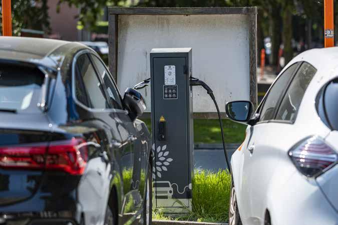
3.2.5 electrification of the transport sector 103
3.2.6 Electrification of heating in buildings 117
3.2.7 Electrification of industry and data centres 126
3.2.8 Sensitivities regarding flexibility 134
3.2.9 Summary regarding load and flexibility 135
3.3 generation and storage 136
3.3.1 Key changes compared with the previous study 136
3.3.2 Non-thermal renewable energy sources 136
3.3.3 Storage 141
3.3.4 Thermal production fleet 146
3.3.5 Outages rates 151
3.3.6 Carbon emissions of the Belgian fleet 152
3.3.7 New capacity to fill the GAP 153
3.3.8 Summary and sensitivities on generation and storage 154
4. EUROPEAN
SCENARIOS
AND ASSUMPTIONS 156
4.1 Scenarios overview 157
4.1.1 Three main storylines for Europe 158
4.1.2 definition of scenarios used for adequacy and EVA 158
4.1.3 Construction of EU-BASE scenarios 159
4.1.4 Construction of EU-SAFE scenarios 160
4.1.5 Additional scenarios used for the EVA 160
4.2 Electricity demand 161
4.2.1 Historical development 161
4.2.2 Adjustment based on 2024 realised figures 162
4.2.3 Relative comparison between countries 162 4.2.4 Electrification of transport 163
4.2.5 Electrification of heat in building 163
8.5
8.5.1
8.5.5
8.5.6
8.5.7
8.6
8.7
8.7.1 EV Flexibility
8.7.2 Stationary Battery Flexibility
8.7.3 Heat Pump Flexibility
8.7.4 Summary of the results
8.8 conclusion of the EVA 281
8.9 Capacity mixes for the flexibility means calculations and for the economic assessment 282
9.
9.1.1
FLEXIBILITY
9.1.4 Specific flexibility challenges
9.1.5 Summary of findings
9.2 Flexibility means
9.2.1 Installed flexibility
9.2.2 Operationally available flexibility means
9.2.3 Contribution of different technologies to flexibility
9.2.4 Sensitivities
9.2.5
• Accelerating the rate at which electrification occurs in Belgium will push the level of demand beyond the level of available capacity from 2028 onwards
• The capacity remuneration mechanism (CRM) remains a cornerstone of Belgium’s adequacy strategy – it keeps vital thermal capacity online while driving investment in new low-carbon assets
• A forward-looking energy strategy for Belgium that includes structural levers could complement the capacity secured by the CRM and close the supply gap
• Flexibility is key: the system needs both responsive consumption and generation to occur in order to manage increasing volatility and periods of oversupply
FOREWORD
KEEPING THE LIGHTS ON IN A FAST-CHANGING ENERGY SYSTEM
Dear reader,
The energy transition is changing at an unprecedented pace, and growing uncertainties are emerging on many fronts. Predicting long-term trends has become more challenging than ever.
Many of the assumptions adopted in our previous studies — especially those related to the electrification of the transport and heating sectors and the rapid deployment of solar PV — have proven accurate and are now being validated by recent developments.
Not all sectors have progressed at the same speed. The energy transition continues to present the sector with surprises. The remarkable growth of battery storage and data centres, for example, has far exceeded expectations. By contrast, forecasts related to industrial consumption levels have yet to materialise, largely due to uncertainties and delays in industrial electrification and broader competitiveness pressures.
PLANNING FOR MULTIPLE FUTURES TO ADDRESS UNCERTAINTY
In this highly dynamic environment, fact-based scenario planning is essential to capture diverging trends. This helps us to provide the best possible insights about our electricity system, as some developments are accelerating while others are unfolding more gradually.
In order to reflect these uncertainties, three distinct scenario frameworks are included in this study for the first time: (1) Constrained Transition (2) Current Commitments & Ambitions and (3) Prosumer Power
Each framework is built around different assumptions regarding policy decisions, technological progress, and societal trends. These are not forecasts, but explorations of how the future energy landscape could change given different conditions.
By using this broader scenario framework, we aim to support policymakers to take more robust and forward-looking decisions about the design and dimensioning of Belgium’s future energy system. Such decisions need to take into account the long lead times required to develop new infrastructure and implement technical solutions.
FLEXIBILITY IS BECOMING CRITICAL ON BOTH THE DEMAND AND SUPPLY SIDES
The growing complexity of the energy system also raises important operational challenges. For example, the level of grid congestion is increasing as connection volumes outpace the development of grid infrastructure, while the rapid expansion of renewables is causing more frequent moments of oversupply to occur.
In addition to storage – of which a significant amount of capacity is already connected to the high-voltage grid - the system will need more flexible consumption patterns and more controllable renewable energy sources. Together, these will both strengthen the system’s resilience and also unlock new opportunities for consumers and market players.
Consumption which has a greater level of responsiveness to the availability of renewables and market prices offers clear benefits. Shifting the consumption of electricity to periods during which high levels of renewable output occur – when
electricity is more abundant and affordable – supports both the stability and efficiency of the system.
Managing renewable generation also plays a key role. Even with more responsive demand patterns, moments will occur when modulating solar or other renewable output will allow suppliers’ portfolios to be optimised and helps to safeguard the stability of the system. This approach is not about limiting renewables, but about enabling their full and sustainable integration into the system in the most cost-effective way.
THE CRM REMAINS KEY, AND MAY BE COMPLETED WITH OTHER STRUCTURAL LEVERS
As Belgium moves towards accelerating its pace of electrification, the need to secure additional capacity will become critical – with new capacity required from 2028 onwards to maintain security of supply. While shifts in consumer behaviour can help to manage peaks in demand, the greater challenge lies in ensuring a resilient, low-carbon electricity supply.
In this context, the CRM remains a cornerstone of adequacy. Without it, there is a real risk that existing thermal assets will exit the market prematurely, and that new investments may fall short – both in terms of scale and timing.
Additional structural levers could be mobilised to complement the capacity that is developed through the CRM. These levers could both address adequacy gaps and also challenges related to gaps in the energy supply. Adequacy and energy supply are two sides of the same coin.
These levers include options such as the lifetime extension of nuclear units or the construction of new units, additional available offshore wind capacity, cross-border capacity and interconnectors, and the structural reduction of demand (through energy sobriety and efficiency measures). Timely decisions about these options would enable the Belgian system to gradually include a more diversified, resilient and decarbonised energy mix.
THE SOLUTIONS ARE ON THE TABLE
This report is a call to deliver. The facts are known, the levers have been identified, and there is political will to shape a longterm energy vision for our country.
Delivering on this vision will require the continued implementation of the CRM, an acceleration of the development of flexibility - both on the demand and generation sidesand greater clarity about long-term choices for the energy mix. Achieving this will require coordinated and sustained efforts from all actors: public authorities, regulators, grid operators, producers, market participants, industrial players, and citizens.
I would like to thank all our experts who once again dedicated their energy and expertise to this report, as well as all of our stakeholders for their valuable suggestions and feedback. I sincerely hope that this report will act as a meaningful contribution to the upcoming discussions that will be held about the shaping of Belgium’s future energy policy. Delivering on this collective commitment is now our shared priority.
Frederic Dunon CEO of Elia Transmission Belgium
WHAT IS THE DIFFERENCE BETWEEN ‘ADEQUACY’ AND ‘FLEXIBILITY’?
‘Adequacy’ and ‘flexibility’ are two key pillars that ensure the secure and reliable operation of any electricity system. Both are essential to maintaining a country’s security of supply. In this study, Elia analyses and quantifies Belgium’s adequacy and flexibility needs for the 2026–2036 period.
Adequacy refers to the ability of an electricity system to meet the demand for electricity in line with the system reliability standards which are set by the government. It therefore relates to ensuring that enough electricity is available to cover consumption levels, even during periods when the demand for electricity is high or during unexpected events — such as extreme weather conditions or when there are disruptions abroad.
A system is considered ‘adequate’ if it meets the national reliability standard, which in Belgium limits the loss of load expectation (LOLE) to no more than three hours per year.
Flexibility, on the other hand, is the system’s capacity to handle expected and unexpected variations in the production and consumption of electricity. These fluctuations are becoming more frequent due to the growing share of variable renewable energy sources (like wind and solar) in the system. At the same time, as electrification spreads across the transport, heating and industrial sectors, new forms of flexible electricity consumption are emerging. These can be activated to balance the system more efficiently, helping to keep it affordable, sustainable, and secure.
As more renewable energy sources like wind and solar are integrated into the electricity system, flexibility becomes increasingly important. These weather-dependent resources cannot be dispatched like conventional power plants. As a result, the system must deal with periods of oversupply, when more electricity is produced than consumed, and power deficits, when there isn’t enough electricity to meet the demand for it.
If these imbalances are not addressed in real time, they can affect grid stability and eventually lead to a blackout. Flexibility is essential for absorbing these fluctuations — by adjusting levels of consumption and/or generation — and for keeping the system balanced, reliable and secure.
CHANGE IN EMPHASIS OVER TIME
This publication marks Elia’s fifth adequacy and flexibility study for Belgium, covering the next ten years.
Whilst the system’s adequacy remains a core pillar in this year’s study, our analyses increasingly highlight the need to include flexibility as a structural component of system security.
For nearly a decade now, Elia has been highlighting the need for flexibility in the system. Currently, that need is more tangible than ever: whilst technologies like battery storage systems are being scaled up, end-user flexibility and modulation of decentralised PV remains underdeveloped and undervalued. Unlocking this potential — through market design, digitalisation, and behavioural incentives — will be essential for harnessing the full benefits of a
system.
THREE SCENARIOS TO ANTICIPATE BELGIUM’S ENERGY OUTLOOK
To ensure a robust and forward-looking assessment of Belgium’s needs, we’ve moved beyond a single-scenario approach to embrace a more diversified methodology. Our analyses now build on three forward-looking scenario frameworks, each of which reflects a different trajectory – ranging from slower transitions to more ambitious, accelerated paces of change.
The scenarios provide a broad yet realistic perspective of how Belgium’s electricity system could change over the next decade. In today’s highly dynamic and uncertain environment, scenario-based planning is essential for capturing diverging trends and emerging uncertainties. It enables us to deliver the most relevant insights into the electricity system, so providing decision-makers with support that remains robust across a wide range of possible futures, as some developments accelerate while others unfold more gradually.
CURRENT COMMITMENTS & AMBITIONS SCENARIO
This is the path Belgium is currently on, assuming that announced targets are indeed implemented across Europe.
This scenario is aligned with Belgium’s current energy policy and announced targets. It reflects official forecasts from the Bureau du Plan, the National Energy and Climate Plan (NECP), recent federal and regional government agreements, and electrification plans from the industrial sector.
CONSTRAINED TRANSITION SCENARIO
This scenario assumes a slower uptake of electric vehicles, heat pumps, and end-user flexibility — as well as delays in the deployment of wind generation, storage and grids across Europe.
This scenario assumes that Europe faces challenging macro-economic conditions. This could slow down the pace of grid development, renewable energy investment, and electrification of industry.
It also considers supply chain difficulties, delays in the implementation of certain policies — like EU Emissions Trading System 2 (ETS2) — and low levels of public acceptance with regard to infrastructure projects, like new grid assets or onshore wind farms.
PROSUMER POWER SCENARIO
This scenario assumes more PV, electric vehicles, heat pumps and enduser flexibility, while the other values are kept the same as in the Current Commitments scenario.
This scenario assumes that current consumer trends accelerate faster than in the Current Commitments scenario. Prices for technologies like PV, home batteries, and electric vehicles continue to fall, making them more accessible to households. In addition, a faster rollout of heat pumps in existing and new buildings, driven by additional policies but also more end-user flexibility is assumed to be available in the system.
METHODOLOGY
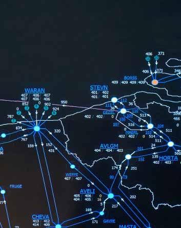
This study includes a simulation of 11 years (from 1 September 2026 to 31 August 2037) for the entire European system – not just for Belgium. This allows the interdependent nature of electricity markets and grid dynamics to be reflected.
Each of these years is assessed against 200 different climate year profiles, meaning weather-dependent generation and consumption is modelled on an hourly basis, under a very broad set of possible conditions. Additionally, a flow-based market model is used for the entire Central Europe Capacity Calculation Region (CCR), ensuring an accurate representation of cross-border flows and network constraints.
Central Europe CCR consists of the
zone borders between the following EU Member States, plus Switzerland’s bidding zones: Austria, Belgium, Croatia, the Czech Republic, France, Germany, Hungary, Italy, Luxemburg, the Netherlands, Northern Ireland, Poland, the Republic of Ireland, Romania, Slovakia and Slovenia.
MAIN CHANGES SINCE THE 2023 ADEQUACY AND FLEXIBILITY STUDY
This report is Elia’s fifth biennial study on Belgium’s adequacy and flexibility needs, covering the period 2026–2036. It builds on the previous adequacy and flexibility study (referred to from here onwards as ‘AdeqFlex’23’), which was published in 2023, and incorporates the latest market trends, policy developments and updated system insights. Several key assumptions and drivers have changed for Belgium since the publication of the last study.
1.
Lower levels of electricity demand and the delayed electrification of industry
Compared with AdeqFlex’23, the projected level of electricity consumption in Belgium is lower. This reflects recent trends, including a reduction in the level of industrial electricity demand and delays to industrial electrification projects.
However, this decrease is not uniform across all sectors. The electrification outlook for the transport and heating sectors remains largely in line with previous projections. In addition, the growth in demand linked to data centres has been confirmed and remains robust.
2.
More electric vehicles, but a slower development of flexibility
Progress continues to be made on the electrification of the transport sector. The Current Commitments scenario of the current study (AdeqFlex’25) now anticipates a slightly higher number of electric vehicles (EVs) being on the road by 2030 than was projected in AdeqFlex’23. However, one important change concerns the level of flexibility unlocked from these EVs.
In light of slower-than-expected market developments – such as the limited uptake of dynamic electricity tariffs – the share of flexible charging is now expected to be lower than previously assumed. A larger portion of EV charging is therefore still expected to occur in an uncontrolled manner (‘natural charging’).
Nonetheless, the growing adoption of tariffs which incentivise behavioural changes and self-consumption (from solar PV) will help foster some degree of flexibility.
3.
Adjusted assumptions regarding the electrification/flexible consumption patterns of industry and data centres
Industrial electrification plans have been slowed down, and recent trends indicate that there has been a reduction in levels of industrial electricity consumption. As a result, the additional level of industrial demand projected in AdeqFlex’25 arises at a slower pace than included in AdeqFlex’23 (brutto). At the same time, flexibility expectations related to larger industrial electrification projects have also been revised downwards, based on feedback collected since AdeqFlex’23 and results collected during recent client surveys.
By contrast, the growth in the level of demand from data centres has been confirmed, and remains an important driver in future load projections.
4.
Delays in the development of offshore wind and interconnector projects
AdeqFlex’23 assumed the development of the Princess Elisabeth zones (PEZ) I, II and III by 2030, including the Nautilus interconnector. In addition, the TritonLink interconnector (linking Belgium to Denmark) was also assumed to be commissioned by 2032.
Rising costs for high-voltage direct current (HVDC) infrastructure and related market uncertainties have delayed the timeline for the development of additional offshore wind capacity in Belgian waters beyond PEZ I and PEZ II, and have also delayed the development of interconnectors.
AdeqFlex’25 therefore explores various sensitivities after 2035 for offshore wind and interconnector capacity between Belgium and other North Sea countries.
5.
New capacities that have been secured as part of the CRM
Since the publication of the previous study, additional (new) capacities have been awarded contracts through Belgium’s CRM. These include new storage projects that are due to be commissioned over the next three years and the lifetime extension of an existing open-cycle gas turbine (OCGT), which were not considered in AdeqFlex’23.
KEY MESSAGES
MESSAGE 1
THE TRANSFORMATION OF THE SYSTEM FACES FLEXIBILITY AND INFRASTRUCTURE CHALLENGES
Belgium’s electricity system is undergoing a profound transformation. Renewables and storage sites are rapidly being expanded, electrification is progressing across sectors, and digital consumption - driven by data centres - is accelerating. At the same time, industries are facing growing competitiveness pressures and delays in the development of critical infrastructure. However, the efficiency of this transition is hindered by the slower-than-expected uptake of end-user flexibility.
MESSAGE 2
THE CRM IS ESSENTIAL FOR SECURING EXISTING AND NEW CAPACITIES, AND MAY BE COMPLEMENTED BY STRUCTURAL LEVERS
Our adequacy assessments confirm that Belgium’s electricity system will remain reliable in the short term, thanks in large part to the various CRM auctions which will begin to deliver capacity from 2025 onwards and the lifetime extension of nuclear units. From 2028 onwards, the CRM will continue to play a key role in the system, since it will help to retain vital ageing dispatchable capacity and support investments in new capacities. Additional structural levers could be mobilised to complement the capacity developed through the CRM. Timely decisions regarding these options would enable the Belgian system to gradually build a more diversified, resilient and decarbonised energy mix.
AdeqFlex’25 2026-2036
MESSAGE 3
FLEXIBILITY ACROSS ALL LEVELS IS KEY FOR MANAGING PERIODS OF OVERSUPPLY AND VARIABILITY
Accelerating the rollout of system-wide flexibility - across consumers, including the residential and industrial sectors – will be critical for ensuring that the system remains efficient, resilient and future-proof. As the levels of renewable generation continue to grow, periods of oversupply will become increasingly frequent. Meeting these challenges will require a balanced combination of solutions: the deployment of storage solutions, increased levels of flexibility from end users, and enhanced levels of flexibility from (decentralised) renewable energy sources themselves. By unlocking the end-user flexibility the consumer wins twice: lower system costs and a lower electricity bill. Further market, regulatory and technical reforms are necessary to enable this.
AN INCLUSIVE AND COMPLIANT APPROACH
INCLUSIVE STAKEHOLDER CONSULTATION
In line with the Belgian Electricity Act, this study was prepared in collaboration with the Federal Public Service (FPS) Economy and the Federal Planning Bureau, and in consultation with the Commission for Electricity and Gas Regulation (CREG). Regular meetings and consultations were held with these institutions from June 2023 onwards.
In addition, a public consultation was held in November 2024, during which stakeholders were given the opportunity to review and to learn about the data and methodology used and different scenarios explored for the study. Following this, Elia received over 100 comments and suggestions from 15 stakeholders.
A wide range of stakeholder proposals were integrated into this study. Firstly, as suggested, the latest data relating to 2024 for all countries was included in the scenario trajectories (amount of RES, EVs, HPs, offshore ambitions, electrification, impact of the energy crisis). Secondly, three pan-European scenarios were developed to reflect the various uncertainties which are currently shaping the energy landscape.
COMPLIANT WITH BELGIAN AND EU REQUIREMENTS, USING UP-TO-DATE INFORMATION
After EU Regulation 2019/943 came into force (in October 2020), the EU Agency for the Cooperation of Energy Regulators (ACER) approved the methodologies for performing future European Resource Adequacy Assessments (ERAA) and national adequacy assessments.
This study is fully aligned with the current legal and regulatory frameworks, including EU Regulation on Electricity Market design (as part of the Clean Energy for All Europeans Package) and the ERAA methodology. The scenarios explored in this study are based on the most up-to-date information that Elia had access to at the end of February 2025. This includes the regional and federal ambitions which are now covered by government declarations or in the Regional/Federal Energy Climate Plans which are due to be integrated into the updated draft Belgian National Energy and Climate Plan, which should be submitted by Belgium in the course of 2025.
This study also includes Europe’s most recent ambitions, policies and targets (e.g. Fit for 55, REPowerEU); Member State plans or ambitions; the most recent offshore wind ambitions and developments for each country; and public announcements (e.g. national unit closures/extensions, historical data); national adequacy studies and bilateral discussions.
CAPACITY OUTLOOK FOR BELGIUM
ADDITIONAL CAPACITY NEEDS OVER THE NEXT DECADE
The figure below illustrates the new amounts of capacity that Belgium will need (assuming a 100% availability level) to meet its reliability standard over the coming decade.
WHAT DOES THE FIGURE ABOVE DEMONSTRATE?
The figure depicts Belgium’s projected capacity needs over the next 10 years, highlighting:
• NEW CAPACITY already contracted through the CRM.
• NUCLEAR EXTENSION - Doel 4 and Tihange 3 until 2035.
• CAPACITY GAP or margin under three different EUSAFE scenarios:
– Constrained Transition (CT);
– Current Commitments & Ambitions (CC);
– Prosumer Power (PP).
These reflect varying assumptions about electrification, levels of renewable growth and flexibility, and the impact of foreign short-notice risks which lie beyond Belgium’s control and responsibility.
• IMPACT OF SLOW FLEXIBILITY UPTAKE – The additional capacity need that could arise if flexibility uptake in the industrial, residential and tertiary sectors is slower than expected.
WHAT DOES THIS MEAN IN PRACTICE?
Electrification across society will drive additional capacity needs to ensure adequacy
• NEAR-TERM MARGIN, BUT NEW NEEDS FROM 2028 – While Belgium is expected to maintain a capacity margin in the near term – supported by the lifetime extension of nuclear reactors and capacities contracted under the CRM – a need for new capacity emerges from 2028 onwards in certain scenarios, and from 2030 onwards in all scenarios.
• LARGER GAP EXPECTED BY 2035 – By 2035, a larger capacity gap is expected to appear as current nuclear reactors (Doel 4 and Tihange 3) reach the end of their lifetime extensions
• FLEXIBILITY REMAINS KEY TO LIMIT CAPACITY NEEDS – The capacity requirements already take into account the development of expected additional consumer flexibility. However, if this flexibility does not materialise, additional volumes of capacity will need to be secured. Specifically, the slower uptake of flexible consumption in the residential, tertiary and industrial sectors could increase capacity needs by approximately +700 MW by 2030 and +1,300 MW by 2036.
THE FOLLOWING ELEMENTS ARE ALREADY TAKEN INTO ACCOUNT IN OUR GAP/MARGIN CALCULATIONS:
GENERATION
all existing generation units (except those officially scheduled for closure);
new capacities secured through the CRM, including new batteries, combined cycle gas turbine (CCGT) plants, and refurbishments;
the lifetime extensions of the Doel 4 and Tihange 3 nuclear reactors (whose operation, at the time of writing, has been approved until 2035);
the additional renewables, including the planned commissioning of the Princess Elisabeth Zone I which is assumed for 2031 (+700 MW) and Zone II which is assumed for 2032 (+1,400 MW).
FLEXIBILITY & STORAGE
the existing level of demand response (considered to fully contribute to adequacy);
the additional amounts of flexibility expected to be developed alongside the spread of electrification (both at residential and industrial levels);
the existing and contracted level of storage in the system amounting 1,500 MW in 2028 the development of small-scale storage accounted for in the scenarios
— To simplify the message, the decreased contribution of existing and contracted batteries to adequacy is not integrated in this chart.
IMPORTS
The contribution of cross-border exchanges to adequacy is captured through detailed, hourly modelling of the entire European power system.
EU-SAFE
Given Belgium’s high dependence on imports, any event happening abroad will have a significant impact on its adequacy requirements. In this study, we therefore take into account several sensitivities like the reduced availability of France’s nuclear fleet, the possible delayed deployment of grid infrastructure abroad or risks of drought that could lead to low levels of hydroelectric production in Europe.
Adopting a prudential approach, Elia recommends the use of the EU-SAFE scenario as a reference for maintaining Belgium’s security of supply. This scenario represents the sensitivity of a reduced availability of France’s nuclear fleet. This is also the scenario that was chosen to calibrate the CRM parameters by the Belgian federal government in the past auctions.
i It is important to note that this adequacy and flexibility study is not a CRM calibration report and does not aim to calculate future auction parameters.
WITHOUT SUPPORT, A LARGE SHARE OF THE EXISTING THERMAL FLEET COULD CLOSE OVER THE COMING DECADE
Our analysis shows that without support mechanisms - such as the CRM - approximately 1,600 MW of existing thermal capacity (mainly old units) is at risk of leaving the market in the coming decade. This is largely driven by the ageing nature of Belgium’s thermal power fleet, with several units soon requiring significant refurbishment to remain operational.
The figure below illustrates the capacity at risk under different scenarios and sensitivities. The values are representative of the entire horizon of the study as economic viability is calculated on the unit lifetime. All values shown represent the nominal capacity.
EXISTING CAPACITY AT RISK OF CLOSURE WITHOUT ADDITIONAL ECONOMIC SUPPORT
WHAT DOES THE FIGURE ABOVE DEMONSTRATE?
• Belgium currently has approximately 7,500 MW of nominal installed capacity from large existing CCGT, OCGT units (including large Combined Heat and Power plants or CHPs), and turbojets (TJ).
• An economic viability assessment is carried out for all these units, excluding those under CRM contracts or with a must-run operation. It evaluates their projected market revenues against their fixed cost requirements for the coming years.
• The figure illustrates the volume of existing capacity that is not economically viable when considering both fixed costs and market revenues.
• The economic viability assessment is conducted iteratively until a tipping point is reached—where all remaining units in the market are financially sustainable under current market conditions.
• The volume shown in the figure represents the capacity that was removed until all remaining units were found to be economically viable.
WHAT DOES THIS MEAN IN PRACTICE?
• CAPACITY AT RISK – Without additional support, around 1,600 MW of existing units (about 20% of the current thermal fleet) could be at risk of closure. This corresponds to 3 to 4 existing CCGTs (of around 400500 MW each). Note that old OCGTs and turbojets are also found to be non economically viable without support.
• IMPACT OF ADDITIONAL NUCLEAR EXTENSION
This at-risk volume could increase to up to 2,400 MW if an additional lifetime extension to a nuclear unit (assumed to be 1 GW in the simulations) is implemented within the simulated period. Indeed, such an extension would further reduce the running hours of existing thermal plants, so widening the ‘missing money’ problem and increasing the likelihood of plant closures.
• CRM REMAINS CRITICAL – The continued operation of the CRM – which addresses the ‘missing money’ problem – is therefore critical. The CRM both supports investments in new capacity and also ensures the retention of existing thermal plants. Maintaining this mechanism is key for preserving the adequacy of Belgium’s system over the coming decade.
CRM WILL CONTINUE TO PLAY A KEY ROLE – STRUCTURAL MEASURES MAY COMPLEMENT IT IN THE MEDIUM TO LONG TERM
CRM auctions are expected to continue fulfilling their role in securing the capacity Belgium requires to meet its adequacy needs in the coming years. However, to address the capacity gap in the medium to long run, additional structural solutions may complement the CRM.
The figure below depicts the volumes for each year which are to be secured through the different CRM auctions (on top of all existing capacity). The figure also outlines potential structural solutions that could be deployed to address the long-term gap — solutions that extend beyond adequacy alone.
WHAT DOES THE FIGURE ABOVE DEMONSTRATE?
The figure builds on the previous one by illustrating the following.
• Remaining capacity needs for each year within the currently approved CRM timeline. It assumes that the CRM continues to fulfill its role by contracting the new volumes of required capacity through Y-1, Y-2, and Y-4 auctions, while also ensuring existing capacity remains in the market.
• An overview of potential long-term structural solutions that could be used to address the capacity gap. These include the lifetime extensions of nuclear units, the integration of Nautilus and PEZ III, additional interconnectors that would link Belgium to other North Sea countries, enhanced flexibility across the industrial and residential/tertiary sectors, and behavioral shifts which are aligned with sufficiency assumptions.
WHAT DOES THIS MEAN IN PRACTICE?
• SHORT-TERM MARGIN – The previous CRM auctions and recent lifetime extensions of nuclear units have successfully secured Belgium’s adequacy needs, leading to a temporary system margin the coming three winters (provided the CRM mechanism is kept to prevent the closure of existing units as a result of ‘missing money’).
• MANAGEABLE MEDIUM-TERM GAP – The annual new capacity gap increase is estimated to be 100600 MW – a volume that can realistically be covered by future CRM auctions, as it is comparable to new volumes that were contracted in the past. However, over time this could become more challenging if a growing share of batteries is selected, given that battery derating factors are expected to decrease over time.
• LONG-TERM CHALLENGES – Decisions regarding adequacy requirements beyond 2035 need to be prepared now. The capacity gap is expected to grow significantly due to the planned phasing out of nuclear power and the current CRM framework has not yet been validated for this period. Complementary measures would also contribute to addressing energy supply needs in the long term.
STRATEGIC ACTIONS REQUIRED ACROSS DIFFERENT TIMELINES
IN THE SHORT TERM
Adequacy is achievable, but requires the careful management of ageing capacity and flexibility
Under the assumptions of this study, system adequacy is achieved in the near term, but requires ageing dispatchable capacity to be carefully managed and the deployment of flexibility to be accelerated. Our simulations show that Belgium can meet its reliability standard through to 2028 if four key conditions are fulfilled:
1. CRM auctions (Y-1, Y-2) continue to secure the required amounts of capacity;
4. the system is able to integrate this flexibility efficiently.
Existing dispatchable (steerable) capacity remains essential for the system’s adequacy in the coming years, but much of it is ageing and will require significant amounts of investment to remain operational.
While these assets are carbon-emitting, phasing them out too quickly would create an urgent need for replacement capacity, which would pose short-term adequacy risks. A carefully managed CO₂ phase-out trajectory is therefore critical for ensuring a secure and timely transition to cleaner technologies.
Integrating existing and new flexibility into the system will play a significant role in ensuring Belgium’s adequacy. It is therefore essential to continuously improve its quantification and ensure its availability through upcoming CRM auctions.
IN THE MEDIUM TERM
Growing adequacy gap as electrification accelerates
From 2029 onwards, electrification significantly increases the need for new capacity. Under the Current Commitments EU-SAFE scenario, an adequacy gap of 900 MW emerges by 2030, rising to around 2,200 MW by 2034.
Compared with AdeqFlex’23, electrification is now progressing more gradually in certain sectors, and higher volumes of storage are assumed to be developed. However, this is offset by:
— lower levels of flexibility from industry and end users;
— delays in offshore wind development and interconnector projects;
For this period, three CRM auctions (Y-1, Y-2 and Y-4) remain to be conducted –meaning that a significant volume of existing and new capacity can still be secured to safeguard adequacy.
IN THE MEDIUM TO LONG TERM
The CRM may be complemented by strategic choices to close Belgium’s long-term capacity gap
In the long run, new capacity will be needed to maintain adequacy in a decarbonising system. While flexible technologies – such as batteries and flexible loads – will fill part of the need, steerable low-carbon generation will become essential for managing long periods during which levels of wind and sunshine are low, particularly during winter.
With increasing levels of flexibility and storage in the system, the effective contribution of storage (derating factor) decreases over time.
A number of technological options, which fall outside of the CRM, could significantly reduce the adequacy gap, including: further lifetime extensions to nuclear units;
— additional interconnection capacity (including through a new interconnector between Belgium and the UK);
— additional levels of renewables and particularly offshore wind capacity;
— sufficiency measures aimed at reducing the level of demand;
Given the long lead times required to deploy the above-mentioned solutions (which fall outside of the CRM), it is essential to start shaping a clear and coordinated vision for the Belgian energy system of the future.
FLEXIBILITY IS GAINING MOMENTUM
A key enabler for affordability and system stability
THE SYSTEM’S SHORT-TERM FLEXIBILITY NEEDS WILL INCREASE IN THE LEAD-UP TO 2036
Belgium’s electricity system will require growing levels of flexibility as variable renewable capacity - notably wind and PV – continues to be expanded. As we approach 2036, the need for flexibility across different time horizons becomes more pronounced:
ATTENTION IS SHIFTING TO THE MANAGEMENT OF SURPLUS ENERGY IN THE SYSTEM
Periods of surplus energy (when renewables and must run generation is higher than the consumption) are becoming more frequent in Belgium and across Europe. This is already apparent today: negative prices are becoming more common — a trend that is expected to intensify in the coming years as renewable energy sources integrated into the system grow.
Flexibility is essential both for addressing scarcity situations and for managing periods during which generation exceeds demand. By enhancing flexibility through controllable demand, cross-border capacities, controllable (decentral) renewable generation and storage, the overall capac-
ity needed to ensure adequacy can be reduced, while also strengthening grid stability and limiting the risks associated with surplus energy.
Building a dynamic and responsive energy system means aligning consumption with renewable production and allowing production to adapt to price signals, so that its output can be reduced when necessary. The controllability of solar power in particular can play a critical role when other sources of flexibility, such as demand side response and batteries, are already being used to their maximum.
ADDITIONAL END-USER FLEXIBILITY CAN DELIVER €350 TO €500 MILLION IN ANNUAL SAVINGS BY 2036 FOR THE BELGIAN ELECTRICITY SYSTEM
Flexible consumption is key for addressing scarcity situations and also for managing periods of surplus. Assuming the electricity system remains adequate, our analysis indicates that sufficient flexibility resources are expected to be available.
WHAT DOES THE FIGURE ABOVE DEMONSTRATE?
The figure illustrates the evolution of the flexibility needs in the Belgian electricity system over the next decade, aimed at managing unforeseen fluctuations in demand and generation. Both upward (need for increase in generation or decrease in demand) and downward (need for decrease in generation or increase in demand) requirements are provided. These needs are categorised into three types:
• slow flexibility (response time of 5 hours);
• fast flexibility (15-minute response);
• and ramping flexibility (5-minute response).
WHAT DOES THIS MEAN IN PRACTICE?
• Flexibility needs are projected to increase with 2 to 2.5 GW in addition to today’s total flexibility needs due to the growth in renewables.
– Slow flexibility: the importance of intraday markets will increase with regard to managing forecasting updates a few hours ahead of real time, with required volumes exceeding 4 GW in 2036.
– Fast flexibility: the need for flexibility that can react within 15 minutes of real time – to cover prediction errors or generation and transmission (HVDC) asset outages – is expected to double, exceeding 3 GW in 2036.
– Ramping flexibility: the ability to react within 5 minutes of real time to manage up- and downwards variations is expected to reach about 0.5 GW by 2036.
• These flexibility needs will need to be covered via sufficient liquidity in intraday markets and balancing markets.
The expansion of battery storage and greater use of consumer flexibility can reduce the need for short-term market interventions to manage sudden fluctuations in renewable energy output.
However, depending on the scenario, it may be necessary to implement measures that ensure this flexibility is available in real time and at all times.
Facilitating end-user flexibility helps to reduce the need for additional balancing capacity (system operation needs) and the cost of additional capacity that needs to be procured through the CRM. This not only strengthens the reliability of the system, but also leads to substantial cost savings, which are estimated to stand between €350 to €500 million annually by 2036. This value is further increased by grid investment gains and the value of consumers reacting to energy market prices.
350 – 500 M€ per year of system gains of unlocking additional end-user flex towards 2036 without accounting potential gains of optimizing grid investments
UNLOCKING FLEXIBILITY STARTS WITH AWARENESS
Unlocking the value of end-user flexibility remains a strategic priority for Belgium’s electricity system. Yet today, many consumers - both industrial and residential – are not fully aware of the value they can create by adopting a flexible approach to their use of electricity.
With the right knowledge, incentives and tools, end users can build solid business cases for electrification, lower their energy bills, and use their flexible assets more effectively, while also contributing to grid stability during critical moments.
To fully capture this value, flexibility must be unlocked across all user segments of the system, both industrial and residential.
Industrial flexibility plays a particularly important role. It can provide large volumes of flexibility at lower activation costs and help stabilise the system during critical periods. Unlocking this potential will require an updated regulatory framework, and closer collaboration with industrial actors to address operational barriers.
Residential flexibility is equally crucial, particularly with regard to helping to absorb surplus levels of renewable production and managing consumption peaks. However, the current application of this remains too slow, and stronger efforts are needed to raise consumer awareness and engagement.
Residential PV modulation is becoming increasingly important to respond effectively to price signals, especially with the growing volume of PV generation. To maintain system balance, appropriate incentives and measures must be implemented.
COORDINATED ACTION TO ACCELERATE END-USER FLEXIBILITY
Unlocking large-scale flexibility requires coordinated efforts across the entire energy ecosystem. Since Elia’s earlier publications, several key enablers have progressed and continue to evolve. Accelerated and improved outcomes will depend on stronger collaboration among all stakeholders.
Empower end users by continuing to enhance end-user knowledge and behaviour, without adding complexity as this is essential to keep it manageable and comprehensible for end consumers.
Providing the right price incentives. Elia seeks to facilitate the development of innovative energy services by commercial parties. A key feature of this facilitation is, next to other relevant price signals (such as day-ahead and intraday markets) the Real-Time Price, which is an evolution of the current imbalance price combined with a price forecast. These price signals should enable suppliers to offer new types of energy contracts to consumers, such as dynamic or fixed time-of-use contracts, which we see emerging in the market. These innovative offers should also be supported by non-static grid tariffs that promote flexibility and encourage optimal energy consumption at times when it’s most beneficial for both consumers and the grid.
Set up the right market design to support market parties in their (innovative) offerings. Industrial clients directly connected to the Elia grid will be able to benefit from the Multiple BRP/Supplier service, which allows different contracts for various assets by appointing separate BRPs/suppliers behind the same head meter. In addition, the Transfer of Energy (ToE) framework enables grid users to leverage their flexibility through a Flexibility Service Provider (FSP), independently of their energy supplier. Starting in 2025, together with the DSOs, we will expand ToE to more customers, including medium and low voltage users.
Deploy enabling infrastructure by ensuring the full deployment of smart meters across all regions in Belgium.
Adoption rate varies between the regions, all DSOs have started the rollout. focusing primarily on consumers with the highest flexibility potential, such as those with electric vehicles, solar panels, or home batteries would facilitate a fast unlocking of the residential flexibility. In parallel, DSOs are finlaising the design of the first release of the supply split enabler that should be implemented by 2027.
Standardise and ensure the interoperability of flexible assets by making these assets ‘flex-ready’ so that they can contribute and deliver flexibility to the system.
SMART FLEXIBILITY COULD DRIVE BIG SAVINGS FOR RESIDENTIAL CONSUMERS
Our analysis estimates the annual savings that end users could achieve — in both commodity costs and network tariffs — by increasing the flexibility of their consumption and production assets over the coming decade.
These estimates focus on long-term structural savings and do not include potential additional gains from participation in intraday or balancing markets or evolutions in grid tariffs.
could be gained from short-term flexibility
WHAT DOES THE FIGURE ABOVE DEMONSTRATE?
The figure illustrates the potential annual financial benefits for individual consumers who actively manage – or ‘flex’ – their levels of electricity consumption and production. These benefits include savings on both commodity prices and network tariffs, such as capacity-based charges.
WHAT DOES THIS MEAN IN PRACTICE?
The range shown reflects different scenarios and years over the next decade. The analysis highlights three key levers through which flexibility delivers value.
1. No injection when negative prices occur – By avoiding injecting PV production into the grid during negative price periods, a consumer can save €40 to €250/year (depending on the scenario and year).
2. Optimising EV charging – By smartly charging an electric vehicle (EV), for example when prices are low or to increase self-consumption (in case of a PV installation), the benefit can reach €170 to €530/ year – the largest single lever shown.
3. Optimising heat pump (HP) usage – By adapting heat pump consumption to market signals (such as prices), a benefit of €20 to €70/year can be captured depending on the comfort that the enduser wants and the weather year.
10
FIGURES REFLECTING THE MOST IMPORTANT ASSUMPTIONS AND RESULTS
1. CHANGES IN BELGIUM’S TOTAL ELECTRICITY CONSUMPTION
The figure below depicts the changes in Belgium’s total electricity consumption in the three scenarios in the lead-up to 2036. A detailed view per sector is provided for the Current Commitments scenario.
2. EVOLUTION OF BELGIUM’S ELECTRICITY MIX
To illustrate the evolution of Belgium’s electricity mix, specific choices regarding the future generation mix were made within the Current Commitments scenario.
While many uncertainties remain, the figure below assumes 2 GW of nuclear generation in operation after 2035 and 5.8 GW of offshore wind capacity as from 2035. In addition, various sensitivities are analysed and can be found in the main chapters of this study.
HISTORICAL AND FUTURE ELECTRICITY MIX
WHAT DOES THE FIGURE ABOVE DEMONSTRATE?
• The demand for electricity is expected to grow over the next 10 years; the pace of growth of this demand will be different depending on the scenario considered. Electrification will be the main driver of growth. Among the three key sectors – industry, transport and heating – the electrification of the industrial and transport sectors are expected to carry the most significant impact.
• Data centres are also emerging as a future driver of electricity demand, particularly given the rise of artificial intelligence and growing levels of digital consumption.
• The adoption of electric heating in buildings remains relatively low due.
WHAT DOES THE FIGURE ABOVE DEMONSTRATE?
• The figure depicts the changes in Belgium’s yearly electricity mix since 1970. Belgium was heavily reliant on oil and coal until the first nuclear reactors were commissioned in the 1970s. Nuclear power then became the country’s main electricity source.
• With the gradual closure of coal plants in the 2000s and 2010s, the share occupied by gas-fired generation in the mix further increased. Nuclear availability impacted the mix in the 2010s.
• Looking to the future, the figure depicts a growing share of renewables and decreasing share of gas-fired generation while taking into account the lifetime extension of nuclear units.
3. RENEWABLE EXPANSION - SOLAR PV & ONSHORE WIND
While solar PV is expected to continue being expanded due to falling costs, the development of onshore wind faces more structural challenges that may limit its future growth.
DOES THE FIGURE ABOVE DEMONSTRATE?
• After an exceptional surge in 2023, solar PV continued to grow in 2024, with the total level of installed capacity reaching more than 11 GW in 2024.
• The installed capacity is expected to reach regional targets of 16.5 GW by 2030, even under the Constrained Transition (CT) scenario, due to the accessibility and cost of solar PV.
ONSHORE WIND
• Achieving regional 2030 targets for onshore wind (CC and PP scenarios) will require a doubling of the historical growth rate over the next five years.
• In the CT scenario, where permitting barriers and public acceptance (NIMBY) issues remain unresolved, the deployment of onshore wind is expected to slow down over time. 4.
EXPECTED CHANGES IN RESIDUAL DEMAND
Residual demand represents the remaining electricity demand after the output is subtracted from renewable sources, nuclear units, and must-run thermal generation.
EXPECTED EVOLUTION OF THE AVERAGE DAILY RESIDUAL DEMAND DURING WEEK-END FOR THE ‘CURRENT COMMITMENTS’ SCENARIO ASSUMING NO GENERATION CURTAILMENT AND PRE-MARKET FLEXIBILITY ACTIVATION
WHAT DOES THE FIGURE ABOVE DEMONSTRATE?
• When residual demand is negative, it this an excess of price-insensitive domestic generation – that is, when non-dispatchable renewables and must-run units produce more than the total load. This surplus must be managed through additional flexible consumption, storage, exports, or a reduction in the level of generation.
• When residual demand is positive, this indicates a domestic shortfall. In this case, additional energy is required from other sources, such as dispatchable thermal units, lower flexible consumption.
WHAT DOES THIS MEAN IN PRACTICE?
Looking ahead, the continued growth of renewables will cause deeper and more volatile residual patterns. More periods of excess are likely to occur around midday, when large volumes of solar PV generation coincide with lower levels of demand.
5. PERIODS WHEN RESIDENTIAL PV CURTAILMENT IS NEEDED FOR SYSTEM STABILITY
As Belgium moves towards establishing a more electrified and renewables-based energy system, managing moments of structural oversupply — particularly during the spring and summer — is becoming a central challenge. During these moments, further curtailing generation is one of the options to keep the system in balance.
WHAT HAPPENS DURING A SUNNY WEEKEND WITHOUT WIND IN MAY 2032 IN ‘DAY-AHEAD’ ? (ILLUSTRATIVE EXAMPLE)
Week-end consumption at noon - GW Production at noon - GW
In this example, around 4 GW needs to be stored in large scale storage; exported or curtailed. + Additional means will also be needed to cope with short term flexibility needs of the system happening after day-ahead
WHAT DOES THE FIGURE ABOVE DEMONSTRATE?
The graphic illustrates the situation on a sunny, windless day of May 2032.
• CONSUMPTION – In a scenario in which electrification progresses following the Current Commitments scenario, the total level of midday weekend demand could reach ~10 GW. Activating different flexible consumption means (industrial flexibility, EVs and residential batteries) could add an additional 3 GW. The demand would then reach 13 GW.
• PRODUCTION – From a production point of view, there are around 3 GW of must-run thermal units (of which 2 GW of nuclear) and around 14 GW of PV generating. This figure excludes wind generation. The production reaches ~17 GW, leaving a surplus (when compared to the demand) of around 4 GW that must be stored, exported, or curtailed.
• FLEXIBILITY NEEDS – While 4 GW are needed (after pre-consumption flexibility has been activated) in this example, additional flexibility might be required to cope with imbalances that arise between the day-ahead market and real- time operations. During these moments, further reducing the levels of generation may be necessary to maintain system stability. 6.
UNLOCKING ADDITIONAL DECENTRALISED FLEXIBILITY DURING HIGH INCOMPRESSIBILITY PERIODS
In 2026, there is a risk that flexibility needs will not be met for around 300 hours. Depending on how quickly battery capacity and end-user flexibility is developed, this number could increase to 600 hours by 2036. These critical periods occur during periods of structural energy surplus. Additional 1.8 GW (in 2026) to 2.5 GW (in 2030) of consumer flexibility and decentral PV flexibility is needed to react in the market to manage system imbalances.
WHAT DOES THE FIGURE ABOVE DEMONSTRATE?
• The figure outlines the flexibility that needs to be unlocked in intraday and balancing time frame to meet system flexibility needs during moments when the risk of incompressibility is high. The values shown already account for flexibility contributions from batteries, end-user flexibility, large-scale renewable generation farms and cross-border flexibility (in the Current Commitments scenario), as well as already takes into account contributions from centralised and decentralised wind power.
• The estimated flexibility needs therefore represent an indicator for the minimum volume that needs to be unlocked from consumer and decentralised PV flexibility. This capacity must be capable of responding to short-term market signals within the intraday and balancing markets.
WHAT DOES THIS MEAN IN PRACTICE?
• The volume of flexibility that needs to be unlocked will amount up to 1.8 GW in 2026, increasing to around 2.5 GW in 2030. This flexibility will need to be unlocked on decentralised PV, or on additional enduser flexibility.
• The need for unlocked decentralised PV can be reduced in the lead-up to 2036, depending on the rate of development of new battery capacity in the system.
• For the sake of guaranteeing system security Elia will closely watch the development of this end-user flexibility. Given the slow development so far, it will have to further assessed if Elia, together with the DSOs, will not have to extend the amount of capacity that can be activated as a last resort via the so called ‘technical trigger” by including additional amounts of PV installations.
7.
EFFECTIVE CONTRIBUTION OF STORAGE TO ADEQUACY
The effective contribution of large-scale storage to adequacy is expected to decrease as more capacity is deployed in Belgium and across Europe.
8.
EXPECTED RUNNING HOURS OF THERMAL GENERATION IN BELGIUM
The expected running hours of gas-fired thermal generation is expected to decrease in the long run. This is due to the increase in renewable capacities. For a country like Belgium that enjoys high levels of interconnection with its neighbours, the running hours of a given technology are mostly driven by its place in the European merit order.
The figure below depicts the required capacity of 4h large-scale batteries which are needed to fully close the adequacy gap identified in the EU-SAFE Current Commitments scenario between 2028 and 2034. The ratio between the nominal battery capacity and the adequacy need responds to the derating factor of the technology – that is, its effective contribution to adequacy.
The merit order is a way of ranking available energy resources for the generation of electricity. It is based on the lowest marginal cost and defines the sequence in which power plants are designated to deliver power, with the aim of financially optimising the electricity supply.
MARKET DRIVEN RUNNING HOURS FOR THE MOST EFFICIENT CCGT, EXISTING CCGT AND OLD CCGT IN BELGIUM IN THE CC EU-BASE SCENARIO
EU-BASE Current Commitments scenario
• In 2028 – 400 MW of additional battery capacity will be needed to fully close the 200 MW adequacy gap. This corresponds to a derating of 50%.
• By 2034 – If the entire gap were to be filled using batteries, an additional capacity of 8,300 MW would be needed. However, this could result in an effective contribution of only 2,200 MW, implying a derating factor of around 25%.
WHAT DOES THE FIGURE ABOVE DEMONSTRATE?
• The figure shows the simulated running hours for the most efficient CCGT, an existing CCGT and an old CCGT unit in Belgium (on average and for the 10th and 90th percentiles).
• Over the next 10 years, the number of running hours will decline for the three types of CCGTs. This decrease can mainly be explained by the increased penetration of renewable energy sources, which is expected to occur both in Belgium and abroad.
9.
CHANGES IN POWER SECTOR CO2 EMISSIONS (INCLUSING IMPORTS) AND CROSS-SECTOR OFFSETS DRIVEN BY ELECTRIFICATION (COMPARED WITH 2024)
Electrification offers up important opportunities for reducing the consumption of fossil fuels, which in turn leads to significant reductions in direct domestic CO2 emissions.
The replacement of internal combustion engine vehicles, gas boilers for residential and tertiary heating purposes and fossil-based heat supplies in industry will lead to a significant reduction in (direct) emissions in these sectors.
The analyses only take the effect of electrification into account. Indeed, there are many other levers that will result in lower CO2 emissions, such as additional energy efficiency or sufficiency measures (changes in behaviour and the use of energy).
EVOLUTION OF CO2 EMISSIONS IN THE BELGIAN ELECTRICITY SYSTEM, EXPRESSED AS DELTA WITH 2024 –
SCENARIO
10. DIFFERENT SCENARIOS LEAD TO DIFFERENT OUTCOMES FOR THE ENERGY SYSTEM IN 2036
The three scenarios presented in this study result in distinct outcomes for the energy system. Each scenario involves different levels of electrification and varying electricity mix choices, which in turn lead to differences in renewable energy shares, net electricity imports, fossil fuel consumption, overall fuel expenditure, and emission reductions.
The figure below outlines indicators across the different scenarios for the electricity and energy systems for 2036. It is built on the changes assumed across scenarios (all other things being equal). The differences are purely driven by what is happening in the electricity system and the impact that electrification has on the other vectors.
OUTCOMES FOR THE ENERGY SYSTEM IN TERMS OF RES E-SHARE, ELECTRICITY IMPORTS, FOSSIL FUEL USE AND CARBON EMISSIONS
Comparison of different metrics for the different scenarios in the year 2036
WHAT DOES THE FIGURE ABOVE DEMONSTRATE?
• IN THE SHORT TERM – Total emissions (domestic and imports) deriving from the generation of power in Belgium are expected to increase and then reduce in the longer term. This is mainly due to additional levels of gas generation, which will increase the CO2 intensity of electricity generation in the lead-up to 2026.
• BEYOND 2026 – CO2 emissions linked to power generation will steadily decrease due to more renewable energy sources being integrated into the system, despite the growing level of electrification.
• The electrification of the mobility, heating and industrial sectors will more than compensate for the additional emissions linked to increased power generation needs.
• The effect of electrification can reduce emissions by more than 9 Mt of CO2 by 2030 and almost 26 Mt of CO2 by 2036 when including carbon capture and storage (CCS) in industrial processes. While CCS is not seen as direct electrification, it requires large amounts of electricity, which is taken into account in electricity consumption.
WHAT DOES THE FIGURE ABOVE DEMONSTRATE?
• RES-E – The share of energy consumption from renewable sources (RES-E) is higher in the PP scenario due to the higher levels op PV generation that are assumed.
• IMPORT – Net imports of electricity across all of the scenarios are similar.
• REDUCTIONS LINKED TO FOSSIL FUELS - The reduction in fossil fuels (which is mainly linked to electrification) is much higher in the PP scenario, in which the heat and transport sectors are more electrified than in the other scenarios. The highest reduction in fossil fuel expenditure (cost of importing fossil fuels for the final energy demand in Belgium) is seen in the PP scenario, as greater electrification reduces the need for fossil fuel imports.
• EMISSION REDUCTION – Additionally, the reduction of emissions is also highest in the PP scenario, as part of which 31 MTCO2 can be saved compared to today thanks to electrification only (and taking into account the increase in electricity required). This corresponds to one third of today’s total emissions in Belgium.
Setting the scene
FIFTH EDITION OF THE ADEQUACY AND FLEXIBILITY STUDY
This report marks the fifth adequacy and flexibility study conducted by Elia over the past decade, and the fourth since it became a legally mandated task, serving as the National Resource Adequacy Assessment (NRAA) for Belgium. The current market conditions, along with the geopolitical and economic context, highlight the importance of these studies in identifying system requirements from both adequacy and flexibility perspectives.
Forward-looking assessments of the adequacy and flexibility of our energy system are more important than ever. Such studies are critical for identifying the major trends that will likely emerge over the next 10 years, enabling all relevant actors to measure, anticipate, support, and help shape the changes that the energy system is undergoing. Given the large number of uncertainties, in addition to the different scenarios, hundreds of simulations were performed covering a large number of sensitivities to allow the reader and relevant authorities to evaluate the impact of certain assumptions.
A BROAD RANGE OF SCENARIOS AND SENSITIVITIES EVALUATED
Key trends identified in previous studies are becoming increasingly significant. These include the ambition to decarbonise the electricity system, the electrification of heat, mobility, and industrial processes, the digitalisation of society leading to higher consumption for data centres, and opportunities to manage the system. Additionally, the continuous rise of renewables, advancements in storage, and developments in flexibility, nuclear partial phase-out coupled with the recent geopolitical context, add further complexity.
To address various uncertainties, including the constraints of the energy transition, technological and cost developments, and the adoption of certain technologies, this study begins with several scenarios for Belgium and Europe. Additionally, changes in parameters are evaluated through sensitivity analyses. The EU context is thoroughly examined due to Belgium’s reliance on imports.
CHANGES IN ENERGY POLICIES SINCE THE PREVIOUS STUDY
Since the publication of the previous study in June 2023, Belgium has a new federal government and regional governments in Flanders and Wallonia. The agreements and certain measures are already integrated into the scenarios. In addition, the recent trends and realised figures of 2024 were taken into account for all countries in Europe.
Over the past two years, two Capacity Remuneration Mechanism (CRM) Y-4 auctions and one Y-1 auction have taken place, contracting new and existing capacity. In addition, a large number of large-scale battery projects are being considered by project developers. The rise of data centres and need for computational power for AI is another key trend observed over the past two years. Acceleration of the adoption of EVs and PV panels are further continuing. Similar trends are experienced across Europe as well.
EXTENSIVE STAKEHOLDER INVOLVEMENT FOR THE SCENARIO AND METHODOLOGY DEFINITION
Each edition of this study shows improvement and engages stakeholders through an extensive public consultation process. Elia would like to thank the stakeholders for their comments and input. This consultation leads to adjustments in the proposed data, scenarios, and methodology.
While the study fully complies with the ERAA methodology, it also goes beyond in certain aspects. The scenarios used are based on the most recent data available for the countries involved.
1.1 BACKGROUND AND REGULATORY FRAMEWORK
1.1.1 THE ORIGIN OF THIS STUDY AND ELIA’S ROLE
As Belgium’s transmission system operator (TSO), Elia plays a central role in enabling the changes outlined above: its electrical infrastructure must be adapted to cope with tomorrow’s challenges. Consequently, the Electricity Act assigned Elia the task of carrying out a biennial study of the Belgian electricity system’s ten-year projected adequacy and flexibility needs.
Elia published the first study of this kind in April 2016. In 2018, the Electricity Act of 1999 (further referred to as ‘Electricity Act’) was modified, and Elia published the first study in line with this modification in June 2019. The current study is therefore Elia’s fifth adequacy and flexibility study, as outlined in Figure 1-1. The two central points of focus of this study - adequacy and flexibility - are both crucial components that enable the electricity system to properly function.
The assessment of the system’s adequacy explores whether the sum of expected available capacities, including electricity imports, is sufficient to meet Belgium’s reliability standard - or the necessary level of adequacy. It should be noted that the current study also assesses the economic viability of needed capacities.
— The assessment of flexibility’ investigates the extent to which this capacity carries the right technical characteristics to cope with future (un)expected variations in power generation (in particular, power produced from renewable energy sources) and demand.
The study is also complemented with results on future economic, sustainability, and electricity mix indicators resulting from the hourly future market simulations used in both assessments.
1-1 — LEGAL FRAMEWORK : BIENNIAL ADEQUACY AND FLEXIBILITY STUDIES
It’s the fifth edition of the study since 2016
Apr 2016
Adequacy & Flexibility 2017-2027
On request of the Minister of Energy’s, an ad hoc study on Belgium’s adequacy and flexibility needs was published in April 2016, followed by addendum in September 2016 as requested by the authorities, after extensive stakeholder consultation.
Jul 2018
Legal requirement in the Belgian Electricity Act
Art. 7bis, §4bis (Elia’s translation into English): “No later than 30 June of each biennial period, the system operator shall carry out an flexibility for the next ten years The basic assumptions and scenarios as well as the methodology used for this analysis, shall be determined by the system operator in collaboration with the Directorate General for Energy and the Federal Planning Bureau and in concertation with the regulator ”
1.1.2 THIS STUDY FOLLOWS THE AMENDED ELECTRICITY ACT OF 1999
This study is based on Article 7bis, §4bis of the Belgian Electricity Act, which states that (Elia’s translation into English):
litical and economic context that Europe is facing. Therefore, the study covers every year from 2026 to 2036.
Art.7bis, §4bis (framework for the study)
“No later than 30 June of each biennial period, the system operator shall carry out an analysis of the needs of the Belgian electricity system in terms of the country’s adequacy and flexibility for the next ten years.
The basic assumptions and scenarios, as well as the methodology used for this analysis, shall be determined by the system operator in collaboration with the Directorate General for Energy and the Federal Planning Bureau and in concertation with the regulator.”
Paragraph 5 of the same article states that the analysis should be submitted to the Minister of Energy and the Directorate General for Energy of the Federal Ministry for the Economy (‘FPS Economy’). In addition, it must be published on the websites of both the TSO and the FPS Economy.
As required by law, this study covers the period from 2026 to 2036, considering uncertainties linked to the current geopo-
BELGIUM’S CURRENT RELIABILITY STANDARD
The reliability standard for Belgium is defined according to the Belgian Electricity Act and related royal decrees (Royal Decree of 4 September 2022 [LAW-1] and Royal Decree of 31 August 2021 [LAW-2]). The definition of the reliability standard for Belgium was established following a set legal process and in compliance with ACER’s ‘VOLL/CONE/RS methodology’ (see explanation later in this section).
Furthermore, as referred to in the “Whereas” Article (4) of ACER’s ‘VOLL/CONE/RS methodology’, “the responsibility to determine the general structure of its energy supply is a Member State’s right”, pursuant to Article 194(2) of the 2009 Treaty on the Functioning of the European Union. A Member State’s freedom to set its own desired level of security of supply is also highlighted in recital (46) of the ‘Whereas’ section of the Electricity Regulation (EU Regulation 2019/943). Pursuant to Article 25(2) of the Electricity Regulation, reliability standards should be set by individual member states and are to be based on the ACER approved ‘VOLL/CONE/RS methodology’.
The methodology used by Elia in this study (as outlined further below in Chapter 2) enables the quantification of indicators which can be compared to the reliability standard values, in order to assess the level of reliability/adequacy and related capacity needs. The reliability standards of Belgium and other countries used in this study are explained in more detail in Appendix H.
In order to address identified adequacy concerns after the year 2025, the Belgian authorities have, over the past few years, developed a legal framework which establishes a market-wide Capacity Remuneration Mechanism (CRM). More information on that mechanism in Belgium can be found in BOX 1-3.
It is important to note that this study is not a CRM calibration report and does not aim to calculate the parameters of future auctions. The goal of this study is to highlight potential adequacy and flexibility challenges in Belgium by quantifying and analysing expected electricity market and system requirements. This study therefore seeks to identify any missing capacity or remaining margin in Belgium over the coming 10-year period, in line with different scenarios and sensitivities.
Moreover, whilst auction parameters do need to be defined in order for Elia to undertake the yearly capacity auctions as part of the Belgian CRM, these parameters are the subject of specific and separate CRM calibration reports. Such reports are prepared for each CRM capacity auction in accordance with the applicable legislation. The CRM scenario framework, auction parameters, and rules are drawn from Article 7undecies of the Electricity Act.
Note that there is currently no legally determined standard for flexibility. However, the analysis and methodology used in this study are based on identifying needs in order to keep the system in balance at all times, which is one of the core tasks of a TSO. In addition, Balancing Responsible Parties (BRPs) are expected to balance their portfolios.
The lack of a specific legally determined standard for flexibility is not to be confused with the minimum criteria that Elia uses for its dimensioning of reserve capacity on Frequency Restoration Reserves (FRR) when covering Load Frequency Control (LFC) block imbalances. This is currently set to cover at least 99.0% of expected LFC block imbalances, as specified in the LFC block operational agreement, approved by the Commission for Electricity and Gas Regulator (or CREG - the regulator). This criterion does not lessen the requirement for the system (and market) to be in balance at all times.
FIGURE
METHODOLOGY FOR CALCULATING THE VALUE OF LOST LOAD, THE COST OF NEW ENTRY, AND THE RELIABILITY STANDARD IN ACCORDANCE WITH THE 2019/943 REGULATION (EU)
On 20 October 2022, ACER approved (ACER Decision 23-2020) the methodology for calculating the value of lost load (referred to as ‘VOLL methodology’), the cost of new entry (referred to as ‘CONE methodology’), and the reliability standard (referred to as ‘RS methodology’) in accordance with Article 23(6) of Regulation (EU) 2019/943 of the European Parliament and Council of 5 June 2019 on the internal market for electricity (recast) (hereafter referred to as ‘Electricity Regulation’). The three methodologies are collectively referred to as the ‘VOLL/CONE/RS methodology’.
The Royal Decree of 4 September 2022 [LAW-1] amending the Royal Decree of 31 August 2021 [LAW-2] and relating to the determination of the reliability standard and the approval of the values of the cost of unsupplied energy (referred to in the EU regulation as value of lost load - ‘VOLL’ or ‘VoLL’) and of the fixed cost of a new entrant (referred to in the ACER methodology as the cost of new entry –‘CONE’), set the reliability standard value for Belgium at 3 hours loss of load expectation on average.
Indeed, in accordance with the commitment made within the framework of decision (EU) 2022/639 of the European Commission of 27 August 2021 concerning the aid scheme SA.54915 – 2020/C relating to the introduction of a capacity remuneration mechanism in Belgium (margin number 28), the Belgian authorities updated the single estimate of VOLL on the basis of a new survey concerning the willingness to pay, in accordance with the ‘VOLL methodology’. Furthermore, new values for VOLL, CONE, and RS were established according to the legal process and in compliance with ACER’s ‘VOLL/CONE/RS methodology’ in the Royal Decree of 4 September 2022 [LAW-1].
The LOLE criterion does not require that, for a given target year, every simulated future state (or ‘Monte Carlo’ year) to meet the criterion individually. Instead, it stipulates that the average LOLE calculated across all simulated future states should comply with the criterion. Consequently, there will be a significant number of simulated future states without any loss of load, while some other future states may experience a loss of load exceeding the average criterion.
Details about the reliability standards for Belgium and other European countries, and how to interpret them, are included in Appendix H.
1.2 STAKEHOLDER INVOLVEMENT
As outlined in Article 7bis §4bis of the Electricity Act, this study was developed through a collaboration between Elia, the FPS Economy, and the Federal Planning Bureau, and in concertation with CREG. Multiple ‘Comité de Collaboration’ (CdC) meetings took place between February 2024 and the publication of this study, as shown in Figure 1-2.
The discussions during these meetings mainly focused on: methodology and improvements; scenarios and data; sensitivities; information sharing with different regions; the public consultation processes (documents to submit, Elia’s answers, etc.); the presentation of the first results.
FIGURE
1-2 — STAKEHOLDER INVOLVEMENT
The stakeholder process starts one year prior to the study publication
Adequacy WG Presentation of the consultation report
* Comité de Collaboration (CdC) - meeting with Elia, the FPS Economy and the Federal Planning Bureau and with CREG as observer.
* Adequacy Working Group (WG) - meeting during which Elia and market parties can discuss the development and evolution of the different mechanisms related to the topic of adequacy.
Elia held a public consultation from 5 November to 5 December 2024 which focused on the input data, assumptions, and methodology used for the present study. Elia voluntarily held the consultation to enhance transparency, strengthen the study’s robustness, and gather valuable feedback from market parties.
This public consultation took place in a complex and rapidly evolving context of the electricity system. The European energy market continues to adapt to the challenges of the energy transition, the lasting impacts of the energy crisis, and the geopolitical tensions caused by the ongoing conflict in Ukraine. In Belgium, the situation has also undergone changes in recent months after the 2024 elections. At the beginning of 2025, a new federal government was formed, and in March 2025, the new federal Minister for Energy published his political note [BEL-1] confirming government declarations (See Section 1.5.2). Meanwhile, the final version of the Belgian Energy and Climate Plan is still awaited by the EC [VRT-1].
In response to this dynamic landscape, to the fast evolution of certain technologies, and given the many comments received during this public consultation referring to sensitivities and
scenarios, Elia has developed three main probable future scenarios for Belgium. These scenarios will be combined with scenarios at the European level and complemented with sensitivities (e.g. variation of one parameter only). The scenario submitted for consultation, which is renamed the ‘current commitments and ambitions’ scenario, is studied together with the ‘constrained transition and ‘prosumer power’ scenarios.
The complete methodology employed for the adequacy and economic viability assessments (which comprises several appendix documents and builds on the methodology employed as part of the previous adequacy and flexibility studies) was also put out for public consultation, together with external studies. Those are detailed in BOX 1-1.
The methodology used for short-term flexibility was employed for the first time as part of the AdeqFlex’19 study; no fundamental revisions have been made to it since. The focus, instead, has been on incremental improvements (such as power-to-x, the role played by interconnections, and end consumer flexibility).
OUTCOMES OF THE PUBLIC CONSULTATION ON SCENARIOS, METHODOLOGY, AND DATA
A public consultation focusing on the data and methodology used for the present study was held by Elia between 5 November 2024 and 5 December 2024. In addition to the scenario data and associated explanations, Elia also submitted the methodology and three external studies for consultation.
Over 100 comments from 15 stakeholders were received, as illustrated in Figure 1-3. The public consultation report and the updated scenario data were presented to market parties during the Adequacy Working Group on 21 February 2025 . The relevant documents and presentations are available on Elia’s website [ELI-1].
FIGURE 1-3 — PUBLIC CONSULTATION DOCUMENTS AND FEEDBACK
Over 100 comments received during the public consultation in November 2024
Documents submitted to public consultation
• Document providing explanations on the input data
• Excel file with detailed input data
• 12 comprehensive methodology appendices
• Study on priced-link electricity demand evolution in Belgium and energy efficiency (PRICED study)
• UGent review of Elia heat pump method and assumptions
• Prof. K. Boudt study on the WACC and the hurdle premiums
? Stakeholders feedbacks
• 12 non confidential replies received
• 3 confidential replies received
• More than 100 comments
Febeliec FEBEG CREG Fluvius CANOPEA COGEN
NegaWatt
ODE Vlaanderen
Bond Beter Leefmilieu
Input data / Generation 3
Input data / Total electricity demand 35
Input data / Renewable energy sources 4 Input data / Cogeneration, biomass and thermal production 5 Input data / Storage 1
Input data / Investment cost 6
Input data / Grid & Flow based domains 1
Input data / Data for other countries 2 Input data / Other topics 1
Public consultation report
• An answer is given to each feedback received
• When possible, feedbacks and answers are grouped together
Methodology / General 2
Methodology / Adequacy study 1
Methodology / Climate years 3
Hurdle rates and Prof. K. Boudt study 4
Assessment of short-term flexibility 4 CRM 1
Scenarios and sensitivities 15 General comments 2
• Each answer has been discussed within the Comité de Collaboration
Elia received numerous comments from stakeholders regarding various sensitivities and scenarios, including their storylines and the inclusion of broader contextual elements. Additionally, Elia noted several remarks on the evolution of the electricity demand, particularly concerning the industry sector. In response to this feedback, Elia undertook two demanding actions:
Firstly, different future scenarios for Belgium were developed (combining several uncertainties/sensitivities under a coherent storyline).
The energy landscape is rapidly evolving amid uncertainties, prompting the creation of three scenarios for Belgium based on macroeconomic conditions, international relations, and economic trends. These scenarios aim to provide insights into potential future landscapes.
Constrained transition: Considering poor macro-economic conditions potentially impacting the affordability of the energy transition, affecting new grid & RES projects, and the decarbonisation of the industry. Considering deglobalisation and scarce supply chains, delays of some policies (e.g. CBAM, ETS2), and limited public acceptance for grid and wind projects. This is translated into a slower uptake of EVs & HPs, reduced and slower industry electrification (including some industry closures), slower uptake of end-user flexibility, and delayed realisation of RES and grid projects.
Current commitments & ambitions: Considering announced targets and policies, previously called ‘Central’ or ‘reference’ scenario. This is the scenario submitted for public consultation in November 2024, adapted with the feedback received during the public consultation and the latest commitments. It follows projections from Federal Planning Bureau for macro-economic evolutions, NECP plans submitted by regions and federal authorities, updated with the latest trends, government agreements, as well as industry electrification plans.
Prosumer power: Considering current trends related to prosumers accelerating further, with prices that continue to further decrease for PV, batteries, EVs, making them even cheaper and more accessible. A quicker transition to heat pumps, not only in new constructions but also across the existing building stock. It considers more residential flexibility. Other targets and ambitions are kept similar to ‘Current commitments & ambitions’ (e.g. industry load, onshore/offshore wind).
Secondly, a thorough review of the electricity demand projections was performed.
An update of TSO-connected clients’ future electricity demand projections (gathered via the ‘Load Management’ exercise), based on bilateral contacts, was conducted. Some customers confirmed their previous trajectories while others adapted them, making it possible to better reflect the actual conditions and expectations of the industry sector in the considered scenarios.
In addition, several other important updates were carried out:
A 2024 ‘reality check’ on the latest data available for various parameters (heat pumps, electric vehicles, PV, onshore wind, small-scale generation, realised 2024 electricity demand, etc.). This allows the use of the latest data and ensures the right starting point for the projections. Note that this check has not only been carried out on parameters of electricity demand, but also on RES installed capacities for all Europe when the data was available.
Desktop studies were conducted jointly with Belgian Distribution System Operators (DSOs) to estimate the electrification of the industry connected at the DSO level.
Energy efficiency in the residential and tertiary sector was reviewed based on the E-CUBE deliverable in the framework of the PRICED study.
Other adaptations based on stakeholders’ feedback were introduced, such as a review of the COP curves for heat pumps (HP) and increasing energy efficiency over time for electric vehicles (EVs).
Comments were also received on sensitivities, including the following suggestions that are covered in this report:
Alternative scenarios, in particular the socio-cultural change like sufficiency; Combining some of the sensitivities to better understand the combined effect;
Impact of macro-economic variables on different sectors (electrification, production, etc.);
Impact of end-user and industrial flexibility; Impact of extending further nuclear generation capacity;
Impact of the closure of certain power plant capacities (CHP, biomass, turbojets, etc.);
— Impact of CO2 limit on CRM participation; Impact of RES development.
Comments received on assumptions abroad, including:
— Impact of the non-availability of several French nuclear reactors;
Impact of non/strict achievements of the FB CEP rules.
Regarding the short-term flexibility, the public consultation was limited to providing clarifications based on the stakeholders’ questions, as there were no requests for modifications of the method or assumptions.
1.3 OVERVIEW OF ADEQUACY STUDIES
1.3.1 BELGIAN AND EUROPEAN ADEQUACY STUDIES
In addition to publishing biennial ten-year adequacy and flexibility studies, Elia publishes several additional adequacy-related studies in close cooperation with external partners.
Elia has been mandated to publish CRM calibration reports which contain the information required for determining the volume to be contracted and the proposed parameters for each CRM auction. This task was assigned to Elia in 2021 following the modification of the Electricity Law of 29 April 1999 relating to the organisation of the electricity market (‘Electricity Act’), and related Royal Decrees. These calibration reports are published in line with the Royal Decree that sets the method for calculating the volume of capacity required and the parameters that are necessary for the organisation of auctions within the framework of the CRM (‘Royal Decree on Methodology’). The Royal Decree on methodology outlines the steps that need to be taken for the definition of scenarios and the methodology that should be followed when drawing up these reports. For further details, see BOX 1-3.
With regards to the strategic reserve the mechanism is no longer in force. In the past, Elia performed a yearly analysis
of the Belgian system’s capacity requirements for the next winter period. This responsibility was assigned to Elia in line with Article 7bis of the Electricity Act. Currently, the European Commission’s approval of the Belgian strategic reserve mechanism has expired; therefore, since 31 March 2022, it has not been possible to contract a strategic reserve. All previously published reports are available on the websites of Elia [ELI-2] and the FPS Economy [FPS-1] .
In addition, Elia collaborates with European colleagues from the European Network of Transmission System Operators for Electricity (ENTSO-E) in order to produce a yearly European adequacy analysis. ENTSO-E has published four ‘European Resource Adequacy Assessments (ERAA) so far, in 2021, 2022, 2023, and 2024 (see Section 1.3.2 for more information). ENTSO-E also publishes Seasonal Outlooks twice a year - in the summer (usually in June) and during the winter (usually in December). These reports analyse potential risks relating to Europe’s security of supply, due to, for example, high/low temperatures and other ‘extreme’ conditions.
1-4 — OVERVIEW OF ADEQUACY STUDIES PUBLISHED BY ELIA AND ENTSO-E
Several adequacy studies provide results for Belgium and complement each other
1.3.2 EUROPEAN RESOURCE ADEQUACY ASSESSMENT (ERAA)
On 1 January 2020, a new Regulation of the European Parliament and of the Council on the internal market for electricity (recast) came into force (EU Regulation 2019/943, henceforth referred to as ‘the Regulation’). This Regulation is part of a legislative package known as the ‘Clean Energy for all Europeans Package’ (CEP).
Chapter IV of the Regulation, which comprises eight articles (Articles 20-27), addresses resource adequacy. Article 24 outlines the required methods for carrying out a National Resource Adequacy Assessment. Article 23 addresses the ERAA, which ENTSO-E is required to publish on a yearly basis. The ERAA methodology was proposed by ENTSO-E (in line with Article 23(6)), after which it was amended and adopted by ACER on 2 October 2020 [ACE-1].
Several elements of the methodology are therefore due to be implemented by ENTSO-E in each ERAA study. In doing so, ENTSO-E must strike a balance between the accuracy of the assessment and feasibility of the targeted improvements. Nevertheless, ACER decided neither to approve nor amend both the first and the second editions of ENTSO-E’s European Resource Adequacy Assessment (ERAA) report ERAA2021 and ERAA2022, and only approved the ERAA2023 for the first time in May 2024. [ACE-2]. The draft ERAA2024 report was submitted by ENTSO-E to ACER on 7 April 2025. The ERAA2023 results and draft ERAA2024 results for Belgium are presented in BOX 1-2.
As outlined in the previous adequacy and flexibility study (AdeqFlex’23), Elia is committed to ensuring that each of its 10-year adequacy and flexibility studies is aligned to the furthest extent possible with both the spirit and the modalities of Article 24 (concerning national resource adequacy assessments) and the more elaborated principles as stipulated in Article 23 (concerning European resource adequacy assessments), with particular attention being paid to Article 23(5) (b) to (m) of the Regulation and to the adopted ERAA methodology.
Elia has performed probabilistic adequacy studies for over a decade. The methodologies it has employed for these have been continuously improved through the involvement of stakeholders from across Belgium. More information on methodological details is included in Chapter 2 of the present study and in the dedicated appendices.
RESULTS FOR BELGIUM IN THE LATEST ERAA STUDY FROM ENTSO-E
The results for Belgium from the two previous ERAA reports are presented here ([ACE-2]).
Investment decisions found in ERAA2023 and ERAA2024 are based on ENTSO-E’s total cost minimisation approach using a reduced set of climate years. Generally, the observed economic decisions found in ERAA2023 and ERAA2024 for the ‘Central Reference Scenario’ significantly rely on a few running hours with very high prices (marginally lower or equal to the Price Cap). Therefore, these decisions might not represent fully credible investor decisions.
In any case, the economic viability results for Belgium confirm that:
Not all existing capacity subject to ‘Lifetime Extension’ will be profitable. This means that additional revenues are important to ensure the economic case of existing units throughout the whole period 2025-2035. No new thermal capacity is expected to appear in Belgium throughout the whole period 2025-2035, especially when relying only on ‘Energy-only Market’ revenues.
Furthermore, the results of ERAA2024 consider the probabilistic characteristics of the planned availability of the FR nuclear fleet over the long-time horizons of 2030 and 2035. This is in line with the EU-SAFE scenario storyline. The LOLE results for Belgium for the ‘Central Reference Scenario’, after an Economic Viability Assessment is performed, are presented below:
The LOLE >3h results found in previous ERAA2023 and ERAA2024 confirm that the CRM is an appropriate and necessary measure to ensure the adequacy levels of Belgium. However, they also highlight that the level of adequacy in Belgium heavily relies on the level of SoS and hence, the assumptions of its neighbours (notably France, Germany,
the United Kingdom), which are beyond Belgium’s control, e.g. regarding the availability of the French nuclear fleet.
ERAA2024 (SUBMITTED TO ACER IN APRIL 2025)
ERAA2023 (APPROVED BY ACER IN MAY 2024)
It is worth noticing that ERAA only considers one ‘central reference scenario’, referred as ‘National Trends’. Finally it should be noted that the input data for ERAA2024 was closed after the call-for-evidence, held between 7 March28 March 2024. The assumptions for Belgium were based on the previous AdeqFlex’23 study and latest information known at that time, from CRM calibration reports and CRM auctions.
FIGURE
1.4 CAPACITY MECHANISMS
1.4.1 CAPACITY MECHANISMS IN EUROPE
A significant number of European countries are now relying on capacity mechanisms to ensure security of supply. The reason for this reliance and the specific designs of these mechanisms vary across different member states. However, it is clear that these member states can no longer depend solely on energy market revenues to secure the necessary level of installed capacity for maintaining supply security.
As illustrated in Figure 1-5, nine countries in Europe have implemented market-wide capacity mechanisms: Belgium, France, Italy, Poland, Ireland, and the United Kingdom for market-wide mechanisms, and Finland, Germany, and Sweden for strategic reserves [ACE-4] . In Bulgaria and Greece, the capacity mechanisms ended in 2020.
In terms of market-wide mechanisms, the capacity mechanism in Great Britain has been active since 2017 and was reapproved in 2019. The mechanism applied in France since 2017
has the particularity of being decentralised; however, it is now proposed to move towards a centralised mechanism. Ireland’s capacity mechanism was introduced in 2017 as part of the Single Electricity Market (SEM) reform. Poland introduced its market-wide mechanism in 2018. In Belgium, the first auctions were held in 2021 with a delivery period of 2025 (see Section 1.4.2). The first delivery of the new Italian capacity mechanism started in 2022.
In Germany, Finland, and Sweden, it is strategic reserves that are currently applied. Portugal and Spain do not currently have a capacity mechanism in place but operate under some long-term legacy contracts, known as targeted capacity payments. However, changes are underway: both the German and the Spanish government intend to implement a new capacity mechanism.
Almost ten countries in Europe have a capacity mechanism
Market-wide – central buyer
Market-wide – decentralised obligation
Strategic reserves
No capacity mechanism
1.4.2 CAPACITY MECHANISMS IN BELGIUM STRATEGIC RESERVE (2014-2020)
The Federal Government introduced a strategic reserve as the first capacity mechanism in Belgium to ensure security of supply from winter 2014-15 onwards. The mechanism was approved by the European Commission in 2018 [EUC-1] until March 2022. The strategic reserve was designed to maintain existing generation units (strategic generation reserve, or SGR) and demand-side response capacities (strategic demand reserve, or SDR) out-of-market as a backup to meet peak demand when the market failed to do so. The overview of the volumes that were contracted out-of-market is detailed in Figure 1-6. From winter 2018-19 onwards, no volumes were contracted under the framework of the strategic reserves and, following the rules introduced in the Clean Energy for all Europeans Packages , the approval of the mechanism was not extended.
A strategic reserve mechanism aims to prevent the closure of existing generation, demand response, and storage assets by keeping them out of the market and offering compensation. The instrument is not adapted to support the development of large amounts of new capacities and is therefore not fit for addressing the upcoming adequacy challenges that Belgium will face in relation to the nuclear phase-out and fast electrification.
From strategic reserve to capacity remuneration mechanism in Belgium
MARKET-WIDE CRM (2021 - …)
Given the significant need for new capacities in the coming years as a consequence of the nuclear phase-out, the ageing of the thermal fleet, developments in neighbouring countries, and widespread electrification, a market-wide CRM mechanism was introduced by law in April 2019 [LAW-3]. The law established the general features of the CRM, which were further complemented by a Royal Decree [LAW-4] and Functioning Rules [ELI-3]. The mechanism was reported to the European Commission in 2020, and after an in-depth investigation, the mechanism was approved in August 2021, subject to certain conditions.
In the context of the energy crisis, Belgium decided to extend the lifespan of two nuclear reactors for a period of ten years. In June 2023, Belgium reached an intermediate agreement with Engie. This agreement had to be notified to the European Commission by the end of June 2023 as part of the Capacity Remuneration Mechanism (CRM). The European Commission confirmed that Belgium could proceed with its CRM, which ensures the country’s security of supply at minimal cost. The mechanism is deemed proportionate, considering the ten-year extension of the lifespan of 2GW of nuclear energy. Design modifications to make the mechanism more robust and climate-friendly were also approved on 29 September 2023 [EUC-2] (indexation of the strike price, temporary exten-
sion of the eligibility period for investment costs from one to two years, and stricter CO2 thresholds).
To lower barriers for participation and support non-fossil fuel technologies, Belgium notified the European Commission on 26 August 2024 of new amendments to the CRM: introduction of Y-2 auctions to increase the participation of batteries, multi-year contract for existing capacities, payback exemption for non-fossil fuel technologies. These amendments were approved on 17 September 2024 by the European Commission [EUC-3].
The first Y-4 auction for the delivery period 2025-26 was held in October 2021, and a ‘re-run’ of the first Y-4 auction was also held in April 2022. A second Y-4 auction for the delivery period 2026-27 was held in October 2022. A third Y-4 auction for the delivery period 2027-28 was held in October 2023. In October 2024, for the first time, two auctions have been conducted in parallel: a Y-1 auction for the delivery period 2025-26 and a Y-4 auction for delivery period 2028-29. In October 2025, three auctions will be conducted, following the introduction of the Y-2 auction principle.
More information on the CRM’s design principles can be found in BOX 1-3.
FIGURE 1-5 — CAPACITY MECHANISMS IN EUROPE IN 2023
Source: ‘Security of EU electricity supply in 2023: Report on Member States approaches to assess and ensure adequacy’, ACER, December 2024. The original figure is adapted to include Great Britain as a country with a ‘Market-wide - central buyer’.
FIGURE 1-6 — OVERVIEW OF CONTRACTED CAPACITY UNDER CAPACITY MECHANISMS
BELGIAN CRM IN A NUTSHELL
General purpose of the Belgian CRM
The Belgian Capacity Remuneration Mechanism (CRM) is the cornerstone for ensuring security of supply in Belgium as from 2025. It involves a centrally organised competitive bidding procedure, which is market-wide and technology neutral. It carries the noteworthy features outlined below: Both existing and new capacities can participate; Projects that require significant amounts of investment can apply for multi-year contracts (a maximum of 3, 8 or 15 years, depending on the level of required investments);
— Three auctions are organised for each delivery period. The auction held four years before the delivery period is aimed at projects that have a longer lead time. The auction held two years before the delivery period mainly aimed at contracting more non-fossil fuel technologies, whereas the auction held one year before the delivery period is ideal for projects that cannot commit to providing capacity a long time in advance (such as the flexibility disclosures from industrial processes);
— The CRM has been open for low-voltage participation since the auctions organised in 2024. The Y-1 auction in 2024 was also the first auction with explicit participation from cross-border capacities from Germany and the Netherlands. Until now, there has been no participation from French capacities due to the negligible Minimum Entry Capacity (MEC) with France;
— The CRM is based on reliability options meaning that revenues collected above a defined strike price need to be paid back in order to avoid windfall profits; It is non-fossil fuel demand side management (DSM) and storage friendly As a first step in the implementation of the EMDR, the Belgian CRM has an exemption on the payback obligation for non-fossil fuel technologies which has been approved by the European Commission.
The purpose of the CRM is to compensate for missing-money problems, i.e. when revenues from energy market and/ or revenues from ancillaries are insufficient to compensate for the relevant costs of the (new or existing) capacity. The CRM addresses this by offering a fixed revenue per MW that contributes to Belgian Security of supply. What is the service to be provided?
Capacity contracted under the CRM must be available during (part of) the delivery period(s) to which it has committed. Availability monitoring will take place during all adequacy-relevant moments, defined as the hours for which the Day-Ahead price surpasses a certain level. Elia may also perform availability tests, which are especially relevant in case a capacity cannot be monitored on a frequent basis.
It is important to note is that there is no interference with the energy market; the latter will continue to operate as usual. The CRM applies on top of current energy market provisions and only aims to supplement normal market behavior – providing all contracted capacity in case of (near-) scarcity.
How can market parties participate?
Each auction is held according to parameters selected by the Minister of Energy based on a collaborative process involving the CREG, the FPS Economy and Elia as well as additional external stakeholders via a public consultation. Detailed information about the CRM and specific auctions are available on the website of Elia, the CREG and the FPS Economy:
— The CREG: https://www.creg.be/nl/professionals/ marktwerking-en-monitoring/capaciteitsremuneratiemechanisme-crm
The FPS Economy: https://economie.fgov.be/nl/themas/energie/bevoorradingszekerheid/elektriciteit/ capaciteitsmechanismen/capaciteitsremuneratiemechanis
Eligible capacities that meet all requirements stemming from article 7undecies, §8 of the Electricity Act, are allowed to participate. Key eligibility criteria include respecting the CO2 emission criteria, the refusal of other variable subsidies during the delivery period and achieving – optionally via aggregation – the participation threshold of 1 MWd of capacity that contributes to Belgian Security of Supply. The contribution to adequacy of each technology is determined via derating factors.
1-8 — OVERVIEW OF THE MAIN STEPS OF THE CRM PROCESS
As illustrated in Figure 1-8, these are the different stages to go through as a participant:
Prior to and as a prerequisite for participation to the auction the participant must successfully complete a prequalification process;
Upon selection in the auction but prior to the delivery period, a capacity contract is signed, and the participant prepares its capacity for delivery (in one- or four-years’ time) while going through a pre-delivery monitoring process
During the delivery period, the participant receives a capacity payment in turn for respecting its availability obligation However, a payback obligation applies under certain conditions and when the strike price is exceeded.
A secondary market is available as a risk management tool to address capacity shortages and/or to valorise excess available capacity.
The past and upcoming Belgian CRM auctions
At the time of publication of this study, the CRM process is entering an intense period:
The first delivery period will occur in 2025-26, for which two CRM auctions have taken place: a Y-4 auction resulting in mainly around 1.7 GW derated of new capacity being contracted (October 2021) and a Y-1 auction resulting in existing capacities and some new storage volume being contracted (October 2024); Three other Y-4 auctions took place over the past few years, leading to new batteries being contracted and the lifetime extension of an existing OCGT; In October 2025, for the first time, three auctions will be held according to the parameters selected by the Minister of Energy in March 2025; In parallel, the auction parameter selection process for the Y-1 auction with delivery year 2027-28, Y-2 auction with delivery period 2028-29, and the Y-4 auction with delivery year 2030-31 is ongoing at the time of publication of this report.
1-9 - OVERVIEW OF THE CRM AUCTIONS
FIGURE 1-7 - ILLUSTRATION OF THE MISSING MONEY CONCEPT
FIGURE
FIGURE
1.5 CURRENT CONTEXT AND EVOLUTIONS
The energy landscape is continuously evolving, influenced by both anticipated and unforeseen trends. Current laws, policies, and economic factors are actively shaping the future of the energy system. Additionally, the costs and advancements in technologies such as energy storage and photovoltaic (PV) systems are driving investment decisions.
Since the publication of the previous study, there have been significant developments in policy and emerging trends. Some of these trends have been confirmed, while others are still unfolding. This section aims to provide an overview of these developments and their impact on the adequacy and flexibility of the energy system. The list is not intended to be exhaustive, but rather to illustrate key developments in recent years.
1.5.1 THE EU CONTEXT HAS GREATLY EVOLVED IN THE LAST TWO YEARS
The European Union (EU) has been shaping its energy policies to transition towards a decarbonised energy system, aiming to achieve both energy security and climate neutrality. The development of the EU’s energy policy is spearheaded by several key ambitions and initiatives.
EUROPEAN CLIMATE TARGETS
Several intermediary emissions targets have been proposed or agreed upon towards 2050: 2020 targets: reducing net GHG emissions by 20% compared with 1990 levels; increasing energy efficiency by 20% and ensuring that 20% of total energy consumption is met by RES [EUC-4]. The EU successfully reduced its emissions by 24% in 2019 and 31% in 2020 (due, in part, to the COVID-19 pandemic);
2030 targets: reducing net GHG emissions by at least 55% compared with 1990 levels [EUC-5], as translated into a set of proposals on climate, energy, transport, and taxation policies by the EC;
2040 targets: reducing net GHG emissions by 90% compared with 1990 levels, as recommended by the EC in 2024 (the EC has not yet made a formal legislative proposal to the European parliament and Member States);
2050 target: reaching net-zero emissions by 2050, meaning that any remaining emissions are counterbalanced by measures that remove GHG from the atmosphere, as legally set in the European Climate Law. [EUC-6].
After reaching the 2020 target, still a long way to go before net zero
POLICIES AND COMMUNICATION SINCE THE PARIS AGREEMENT
Since the Paris Agreement in December 2015 to limit global temperature rise to well below 2°C, with efforts to restrict it to 1.5°C, the EU has implemented various policies and communications to address climate targets. Key milestones include (non-exhaustive list):
December 2019: Presentation of the European Green Deal and adoption of the ‘Clean Energy for all Europeans’ package;
September 2020: Presentation of the 2030 Climate Target Plan communication, followed in July 2021 by the adoption of the EU Climate Law, setting a binding objective for climate neutrality by 2050 and a target for reducing net GHG emissions by at least 55% by 2030;
— July and December 2021: Presentation of the ‘Fit for 55’ legislative package, consisting in a major review of relevant EU legislation on climate and energy to meet 2030 and 2050 targets;
March and May 2022: Proposal and publication of the REPowerEU plan, which aims to reduce and phase out the import of Russian fossil fuels by ensuring Europe access to alternative energy sources;
October 2023: Adoption of the final pieces of legislation of the ‘Fit for 55’ legislative package, which includes updates to directives on energy efficiency (EED), renewable energy (RED), EU emissions trading (ETS and new ETS2), and the new Carbon Border Adjustment Mechanism (CBAM);
December 2023: Agreement regarding a reform of the EU’s electricity market design (EMDR) achieved, including the recognition of capacity mechanisms as integral part of the electricity market design, and providing measures to help unlock flexibility;
February 2024: Commission communication recommending the introduction of a 2040 emissions reduction target to set the path to climate neutrality in 2050; political agreement regarding the Net-Zero Industry Act achieved;
June-July 2024: Re-election of Ursula von der Leyen as Commission President, who presents the European Prosperity Plan for sustainable competitiveness;
September 2024: Report on European competitiveness by Mario Draghi focusing on innovation, decarbonisation, competitiveness, and security;
— January 2025: Communication on a Competitiveness Compass incorporating recommendations from the Draghi report to enhance innovation, decarbonisation, and security;
February 2025: Communication on a Clean Industrial Deal to drive growth through decarbonisation, focusing on energy-intensive industries and the clean-tech sector; February 2025: The adopted Action Plan for Affordable Energy proposing measures to lower energy costs, complete the Energy Union, and ensure energy price stability;
February 2025: First Omnibus package on simplification, aiming to reduce complexity of EU requirements, notably for small and medium enterprises (SMEs) and small midcaps (SMCs), e.g. for CBAM;
— March 2025: Commission report on capacity mechanisms, assessing the possibilities of streamlining and simplifying the process of applying a capacity mechanism, including by reviewing the ERAA methodology; June 2025: The European Commission published a guidance on anticipatory investments for forwardlooking development of electricity networks.
ONGOING DISCUSSION AND UPCOMING INITIATIVES
The ongoing discussion and upcoming initiatives focus on ambitious sector-specific action plans, such as those for the automotive, steel, and chemicals industries, aiming to significantly reduce emissions by 2050.
In 2025, the EU plans to set up an Energy Union Task Force to enhance coordination and governance across the Energy Union. By June 2025, the European Commission will also adopt the Clean Industrial Deal State Aid Framework (CISAF) to address clean industrial investments and capacity remuneration mechanisms [EUC-7]. The Commission will also provide guidances on network charges, including to harmonise and reduce them via the use of public budgets. These guidances are aimed to incentivise electrification and flexibility. Later this year, the Commission will offer guidance on Contracts for Difference (CfDs) and flexibility remuneration in retail contracts, and propose the Industrial Decarbonisation Accelerator Act to address permitting bottlenecks and promote low-carbon products. The Electricity Directive will also be reviewed by year-end.
In July 2025, the European Commission will also make a proposal for the upcoming EU budget (the Multiannual Financial Framework or MFF) which will be of relevance for the Connecting Europe Facility for Energy (CEF-E) which is among others used to support investment of cross-border relevance in interconnection and smart grids.
By the end of 2025, it is expected that the European Grid Package will be introduced to speed up the grid build-out, including via amendments to the trans-european network for energy (TEN-E) regulation, via simplification, faster permitting, funding and digitalisation. In 2026, an Electrification Action Plan and Heating and Cooling Strategy will support ambitious decarbonisation goals. A White Paper on electricity market integration and revisions to the EU energy security regulatory framework should be adopted. Legislative proposals should extend the Carbon Border Adjustment Mechanism (CBAM) to other sectors at risk of carbon leakage. The Electricity Regulation might also be reviewed in 2026, and by end of the year, Public Procurement Directives should be revised to include non-price criteria.
FIGURE 1-10 - HISTORICAL EUROPEAN GHG EMISSIONS AND ANNOUNCED TARGETS
1.5.2 THE BELGIAN CONTEXT HAS ALSO EVOLVED SINCE 2023
When looking at Belgium, the context has also changed in the past years and months. Governments were formed in Flanders and in Wallonia, as well as at the federal level. At the time of writing this report, no agreement had yet been reached for Brussels. Looking at the available governmental declarations, several elements were pushed forward with respect to energy and climate. Here are a few examples (non-exhaustive):
At the federal level, electricity cost mitigation for industry (‘energy norm’ for companies, plans to adapt the electricity tariff, support for green investment in industry such as flexibility, CCUS, and energy efficiency), change in taxes for residential and tertiary heating devices (lower VAT on
heat pumps and higher VAT on fossil fuels), and a push for nuclear power plants (extension of existing plants and new ones);
In Flanders, increased onshore wind and PV 2030 targets, support for the electrification of industrial processes, and support for flexibility and smart grid management;
In Wallonia, acceleration of the smart meter roll-out, new mechanisms to support the development of renewable energy, exploration of industry flexibility, and a push for residential and tertiary flexibility;
In Brussels, renovation of buildings (existing and new) will be a key challenge for the next government. FIGURE 1-11 — KEY POLICY EVENTS AND DECISIONS (FOCUSSING ON THE FEDERAL LEVEL)
Navigating energy policy: key federal decisions from 2020 to 2025
The energy and climate policies in Belgium are evolving rapidly. At the federal level, the government aims to balance reducing energy consumption, expanding reliable energy capacity, and enhancing the competitiveness of Belgian industry. This includes aligning with European goals to reduce greenhouse gas emissions by 55% by 2030 and achieve climate neutrality by 2050. The federal government is also advocating for a coordinated European approach to address the competitive disadvantage Belgium faces in terms of energy prices for industry.
In addition to federal initiatives, regional governments in Flanders and Wallonia are also pushing forward with ambitious energy and climate plans. Flanders is focusing on increasing onshore wind and photovoltaic (PV) targets for 2030, supporting the electrification of industrial processes, and enhancing smart grid management. Wallonia is accelerating the roll-out of smart meters, developing new mechanisms to support renewable energy, and exploring industry flexibility. These efforts reflect a comprehensive approach to energy and climate policy across Belgium’s regions.
SOME RELEVANT QUOTES (NON-EXHAUSTIVE) FROM THE FEDERAL AGREEMENT THAT IMPACT THE ASSUMPTIONS MADE FOR THIS STUDY: TRANSLATED FROM THE ORIGINAL FRENCH OR DUTCH TEXT
The government will strive to further develop another key asset in terms of knowledge and experience: offshore wind energy. In cooperation with the regions, the government will pursue an ambitious policy to increase the share of offshore energy, including exploring opportunities beyond our territorial waters. […]
Nuclear energy is an important component of the future energy mix as a carbon-neutral energy source. Under the conditions stated above (sustainability, safety, cost optimisation, etc.), we aim for a share of 4 gigawatts of nuclear energy in our electricity mix. […]
Electric cars not only contribute to the sustainable transition in the fight against climate change, but they can also provide additional flexibility within the electric grid. […]
The government will work with the regions to develop a cooperation agreement for demand flexibility in order to contribute to the development of a robust and stable regulatory framework. […]
To this end, we are strengthening electrification and reducing our dependence on imports [...]
Interconnections (in the wide sense of the term) are an essential element of our energy vision. […] The federal government will plead for a european policy supporting leverage in terms of financing and public support to transport network and interconnexions, to strengthen security of supply in Belgium.
To support our companies, we will increase the tax deduction for investments and broaden it to all investments that give an impulse to the energy and climate transition.
1.5.3 ELECTRIFICATION: CURRENT STATUS AND KEY BENEFITS
ELECTRIFICATION IS STAGNATING IN EUROPE, WHILE ALL STUDIES AND PLANS AIMING TO AT LEAST DOUBLE THE RATE BY 2050
Electrification of Europe’s energy system has stagnated, with 80% of final energy needs still met by fossil fuels. A similar trend is observed in most countries around the world. China has demonstrated remarkable growth in recent years, outpacing both the US and Europe and continuing to expand. Furthermore, numerous studies indicate that achieving carbon neutrality requires a higher rate of electrification, which also provides various additional benefits
— lower emissions for end-uses;
— cost savings and resilience to external shocks;
— reduced import dependency; opportunities for additional consumption flexibility; improved air quality and overall quality of life.
Before the Russian invasion of Ukraine, it was believed that achieving climate goals, energy security, and affordability simultaneously was impossible. However, recent events have shown that electrification can address all three aspects. Geo-
political tensions and supply chain disruptions have shifted the focus from climate change to energy security. Electrification reduces reliance on fossil fuels, diversifies supply sources, and supports climate objectives by lowering greenhouse gas emissions. As renewable energy technologies advance, electricity costs become more competitive, enhancing affordability. Thus, electrification is a comprehensive solution to Europe’s intertwined energy challenges.
With these objectives in mind, the European Commission’s Clean Industrial Deal sets a clear target: achieving a 32% economy-wide electrification rate by 2030. This marks a significant increase from the current rate of approximately 20%.
This target supports broader goals of reducing energy costs, fostering clean technology innovation, and strengthening energy security across the EU. It also aligns with legislative initiatives such as the Industrial Decarbonisation Accelerator Act and reforms in electricity grid infrastructure.
1-12 - ELECTRICITY AS SHARE OF FINAL ENERGY DEMAND
Electrification of final demand stagnated in the European Union, recent proposed plans would require a rapid acceleration
REDUCES EMISSIONS AND IMPORT DEPENDENCY
Electrification plays a crucial role in reducing CO2 emissions due to two main properties. Firstly, the electrification of fossil fuel uses typically requires lower primary energy. Secondly, the source of electricity can be fully decarbonised by relying on renewable and/or other low carbon sources of energy.
The replacement of internal combustion engine (ICE) vehicles, gas and oil boilers for residential and tertiary heating, and fossil-based heat supplies in industry leads to a significant reduction in emissions in those sectors.
Figure 1-13 illustrates the difference in energy (imports) and emissions for supplying 1 million households with a heated home all year round. Switching from gas or oil boilers to heat pumps does increase the overall electricity requirements. However, even if that electricity would be supplied via gas, there are major gains in terms of emissions and energy dependency (reduced imports).
FIGURE 1-13 - HEATING 1 MILLION
Electrification of heating reduces the need for fossil fuel imports and emissions, even in the most pessimistic cases
ELECTRIFICATION INCREASES RESILIENCE TO EXTERNAL SHOCKS
In addition to the previous paragraph, electrification increases the resilience of the Belgian/European system as it would rely less on imports. Costs are also reduced, as most studies have shown. In order to illustrate the resilience of the system, the energy bill for Europe is shown in Figure 1-14. As can be seen, the bill more than doubled from 2021 to 2022.
Furthermore, the impact of electrifying all transport and heating in buildings is added so that we can understand what could be saved via electrification of these two segments. The result is that up to 40% of the energy import bill could have been saved if the current fossil-based transport and heating in buildings had been electrified.
The energy crisis more than doubled the EU’s fossil fuel import bill, electrification of buildings & transport could have avoided up to 40%
FIGURE
FIGURE 1-14 - ANNUAL FOSSIL FUEL IMPORT BILL FOR THE EUROPEAN UNION
1.5.4 ELECTRIFICATION OF RESIDENTIAL USES
ELECTRIFICATION TRANSPORT IS ON TRACK IN BELGIUM
Despite the overall uptake of Battery Electric Vehicles (BEV) in Europe have stagnated Europe since the end of 2023, with first sings of some rebound in early 2025. Belgium has however, maintained a strong upward trajectory, continuing its S-curve-like adoption pattern and evolving from a laggard to a forerunner in terms of BEV adoption. By early 2025, approximately one-third of all newly registered passenger cars in Belgium were fully battery electric, marking a significant milestone in the country’s transition to cleaner mobility. Notably, the increase in BEV sales exceeded projections made in the previous AdeqFlex’23 study, highlighting Belgium’s accelerating momentum in this sector.
As of March 2025, Belgium ranks as the fourth largest BEV market in the European Union, both in relative terms and in absolute numbers. It has overtaken larger countries such as Spain and Italy in total BEV registrations, a remarkable achievement given its smaller population. This rapid growth is largely fueled by the corporate fleet sector, where new company car purchases are increasingly electric due to favorable fiscal incentives and tax benefits. These incentives have made BEVs a more attractive option for businesses aiming to reduce their carbon footprint.
This trend is expected to persist in the coming years, supported by the ongoing greening of the company car fleet and the steady expansion of Belgium’s public and private charging infrastructure. Together, these factors position Belgium as a frontrunner in the EU’s electric mobility transition [EUC-8]. FIGURE 1-15 - HISTORICAL BEV SHARE IN NEW PASSENGER CAR IN BELGIUM AND THE EU
Heat pump uptake slowed down in 2024 when compared to the exceptional 2023 year. Fossil fuel boilers sales representing over 85% of the sales
ELECTRIFICATION OF HEAT IN BUILDINGS IS STAGNATING
Hydronic heat pump (air-water and ground-water) sales as a share of new heating installations have slowly increased from around 5% in 2018 to more than 20% in 2023. Between 2022 and 2023, hydronic heat pump sales even increased by 68%, while total heating appliances sales fell by 20%.
Recent figures illustrate that 2024 saw a decrease in the number of heat pumps sold in Belgium. According to the Climafed federation, the reason for the fluctuation can be explained by the Ukraine war and subsequent elevated gas prices, which led to a very strong instantaneous increase in heat pump orders in the second part of 2022. This short-term effect caused supply chain issues, due to which many of these installations were completed only in 2023.
The primary factors driving the adoption of heat pumps today include regulatory requirements, particularly for new constructions. However, for widespread voluntary adoption, the most significant factor is the cost-effectiveness of these units, which is largely influenced by the full ratio (including taxes, VAT and other costs not related to commodity or grid) between the residential electricity and gas prices. As shown in Figure 1-17, Belgium has the highest ratio of electricity to gas prices among all European Union countries, considering all energy costs, grid fees, and taxes. This ratio is expected to change with the introduction of the new carbon emissions trading system (ETS-2), as gas consumed for heating in buildings will also incur costs for carbon emissions (together with
road transport and small industries). Additionally, it is important to note that a portion of the energy bill consists of various taxes and fees, which explain the main electricity-to-gas ratio across the different countries.
With a COP performance of around 250-350%, heat pumps in Belgium are generally more expensive to run for the user than a gas boiler, and their CAPEX is also typically higher. However, all studies show that the rise of heat pumps is crucial for achieving carbon neutrality at a lower cost. Other benefits of using heat-pumps, such as energy dependence and air quality, have also been highlighted in previous sections.
Source: EUROSTAT
FIGURE 1-17 - RESIDENTIAL ELECTRICITY TO GAS (ALL INCLUDED) RATIO IN EUROPE (S1 2024)
1.5.5 DATA CENTRES AND AI
AI IS EXPECTED TO REQUIRE A LARGE AMOUNTS OF ELECTRICITY
The rise of artificial intelligence (AI) in Europe has been remarkable, with increasing adoption across various sectors such as healthcare, finance, and manufacturing. The impact of this growth on electricity consumption is profound. Data centres in Europe currently account for about 3% of the continent’s total energy consumption, a figure that is expected to increase significantly in the coming years. This surge in energy demand poses challenges for the European power grid, which
CONSUMPTION
must accommodate the increased load while also transitioning to more sustainable energy sources. The introduction of AI-driven data centres further complicates this scenario, as they require not only more power but also more sophisticated infrastructure to ensure efficient and reliable operation. Addressing these challenges will be crucial for Europe to fully harness the potential of AI while maintaining energy sustainability and grid stability.
FIGURE 1-18 - PROJECTED DATA CENTRE DEMAND IN GW (EXCLUDING CHINA AND CRYPTO)
Global projected data centre demand is expected to double in next 4 years mainly driven by generative AI growth
1.5.7 RENEWABLE EXPANSION
SOLAR PV EXPANSION IS EXPECTED TO FURTHER INCREASE WITH LOWER PRICES
Since 2019, the installation rate of solar PV systems in Europe has shown impressive growth, with about 20 GW installed per year. This set the stage for further expansion, as investments and supportive policies were ramped up.
By 2021, this growth continued, reflecting an accelerated adoption driven by increased governmental incentives and decreasing solar PV costs. The energy crisis in 2022 further amplified the urgency for renewable solutions as an answer to the rising energy prices and growing concerns over energy security, leading to a substantial surge in installations. In 2023, the installation rate reached new heights, with approximately 60 GW of solar PV capacity installed across the EU. Moving into 2024, despite occasional policy changes, the EU continued to see robust installation rates. Despite falling installation costs, the current oversupply of PV modules—particularly from China—means that installation rates across Europe are expected to remain steady. However, the resulting downward pressure on daytime electricity prices could challenge the economic viability of new solar projects. To mitigate this, future installations should emphasize modularity and adaptability and users rethink their consumption patterns if technically feasible.
FIGURE 1-20
BATTERY STORAGE CAPACITIES ARE EXPECTED TO FURTHER GROW
Europe’s battery storage capacity has experienced remarkable growth in recent years, driven by decreasing costs and various applications. While storage systems can be installed at different levels (utility-scale, commercial, and residential), the residential storage segment has been the primary driver
of growth in the European battery market, accounting for 70% of the market in 2023, according to SolarPower Europe [SPE-1]. However, in the future, a large portion of storage is expected to come from large-scale installations with several gigawatts of projects in the pipeline.
FIGURE 1-19 - HISTORICAL EVOLUTION OF THE STORAGE CAPACITY IN EUROPE
Storage in batteries is expected to triple in Europe in the coming 5 years
RENEWABLE GENERATION SHARES ARE STEADILY INCREASING
When looking at the hourly share of renewables, a clear trend can be observed over the past decade. The rise of PV and wind generation (both onshore and offshore) in Belgium has led to more hours when the share of renewables is significant. While the renewables have increased, the electricity demand has stagnated, leading to higher shares of renewables. In 2023, several hours experienced a share of PV and wind over 90% of the electricity consumption during that hour in Belgium.
In 2024, those hours further increased. In addition, it can be observed that even though the shares increase, there are still moments where, for several days in a row, low shares of renewable generation are experienced (mainly in winter during low wind periods). This high variability leads to high spreads in electricity prices (both low prices when there is an excess and high prices when there are fewer renewables).
In 2024, Belgium experienced over 10 days when the share of wind + PV exceeded 90% of the demand for at least one hour
Source: ENTSO-E Transparency platform
FIGURE 1-21 - HIGHEST HOURLY SHARE OF PV + WIND IN BELGIUM FOR EACH DAY SINCE 2015
1.5.8 EVOLUTION OF ELECTRICITY MARKET PRICES
PRICES HAVE DECREASED BUT REMAIN HIGH WHEN COMPARED TO PRE-COVID TIMES
In 2022, Europe experienced an unprecedented surge in wholesale electricity prices, reaching levels never seen before. This dramatic increase was primarily driven by the sharp escalation in gas prices, a direct consequence of the ongoing Russian invasion of Ukraine. Given the significant role of gas-fired power plants in electricity generation, the hike in gas prices led to a substantial rise in electricity costs.
1.5.9 GRID DEVELOPMENT IS CRUCIAL FOR THE ENERGY TRANSITION
Additionally, other factors exacerbated the situation, including reduced nuclear output in France due to maintenance issues and lower hydroelectric production across Europe caused by unfavourable weather conditions. These combined factors created a perfect storm, pushing electricity prices to historic highs.
Since the unprecedented peaks observed in 2022, prices have somewhat decreased but remain significantly higher than pre-crisis levels. This persistent elevation in prices poses a challenge for European industries, as they face higher operational costs compared to their counterparts in other regions of the world. The disparity in energy costs can lead to a competitive disadvantage for certain sectors, potentially impacting their global market position.
CRAVING FOR FLEXIBILITY: THE RISE OF NEGATIVE PRICES ON THE SPOT MARKET
While energy prices reached unprecedented levels in 2022, driven by high methane prices, there are more and more low electricity prices being observed in the European market. The rise of negative prices on the spot market has become a notable trend in recent years, driven by the increasing penetration of renewable energy sources such as solar and wind. These negative prices occur when the supply of electricity exceeds demand, often during periods of high renewable generation. For instance, in 2024, Europe experienced a record number of negative price hours, with a 58% increase compared to the previous year. In addition, the number of negative prices on the day-ahead market has also risen sharply. While before 2020, Germany was the main country experiencing around 100 hours with negative prices a year, most European countries are now experiencing them. In 2024, over 400 hours were observed in Belgium, as illustrated in Figure 1-22. These hours can lead to challenges in the electricity system management. The hours also show that there is a lack of flexibility on
both the generation (must-runs) and consumption (demand response) sides.
This phenomenon is particularly prevalent during daylight hours when solar generation peaks. The high variability in renewable energy output leads to significant fluctuations in electricity prices, with low prices during periods of excess generation and high prices when renewable output is limited.
The impact of negative prices on the spot market is multifaceted. On one hand, it highlights the need for greater flexibility (consumption and renewable production) in the energy system to accommodate the intermittent nature of renewable sources. This includes investments in production modulation, energy storage solutions, demand response mechanisms, and grid infrastructure enhancements. As the energy market continues to evolve, addressing these challenges will be crucial to ensure the stability and sustainability of the electricity grid while maximising the benefits of renewable energy.
“A central element in accelerating decarbonisation will be unlocking the potential of clean energy through a collective EU focus on grids. If there is one horizontal area in the energy sector whose importance cannot be overstated, it is the EU’s energy grids.” – The future of European competitiveness by Mario Draghi.
The building of grid infrastructure fit for purpose is critical to enable society’s ambition to accelerate the energy transition. Since areas with high amounts of renewable energy sources (RES) are often remote, the need for long-distance electricity transmission is rising. Moreover, areas with complementary production patterns need to be connected as the availability of RES is not equally distributed across Europe.
To make optimal use of the continent’s RES, Europe needs to facilitate and set up frameworks for partnerships between countries with different levels of RES potential and complementary load and production profiles. The development of cross-border interconnection capacity, both onshore and offshore, is essential in facilitating a pan-European integration of renewable electricity, also in the countries that are short on domestic renewable production.
For the offshore aspect, there is a need for efficient planning across countries to allow electricity to be exchanged between countries whilst also connecting them to offshore wind farms. The high-voltage grid is therefore playing a key role in ensuring secure access to electricity for all citizens while keeping the costs of the system as low as possible.
An appropriate set of investments is to be realised in order to enable and maintain market integration, as well as contributing to overall security of supply. The construction of grid infrastructure has a longer lead time than renewable energy projects [IEA-1]. Therefore, to make the energy transition a reality and reap the most benefits from it, it is in society’s interest that the required transmission infrastructure is built in time.
In Belgium, Elia is responsible for writing and publishing a Federal Development Plan (FDP) for the country’s electrical transmission system every four years. Each plan covers a period of ten years, identifying grid needs, covering these needs by infrastructure or non-infrastructure solutions, along-
side an explanation of the assumptions and methods used to calculate them. As such, it includes the investment program for the (extra-)high voltage grid (110 kV to 380 kV) that Elia will implement to meet the identified needs.
As Elia develops each plan, it works closely together with different actors across society, and ensures the plans are aligned with national policy. The FDP is approved by the Minister of Energy before being officially adopted. The latest FDP covering the period 2024-34 was approved in May 2023 [ELI-4] and the next version covering the period 2028-38 is set to be published in 2027. Given that Elia also owns and operates the local transportation grids in the different regions (30 kV to 70 kV), a similar process of developing regional investment plans exists for Flanders, Wallonia, and the Brussels Region.
At the European level, ENTSO-E’s Ten-Year Network Development Plan (TYNDP) is a reflection of each Member State’s national development plans with a focus on (hybrid) interconnection projects. It looks at the whole of the future power system and assesses how power links and storage solutions can be used to make the energy transition happen in a cost effective, sustainable, and secure way.
The TYNDP describes a series of possible energy futures which are developed in collaboration with ENTSO-E’s gas counterpart, ENTSO-G, and a number of environmental and consumer associations, the energy industry, and other interested parties. These processes use a methodology for cost benefit analysis approved at a European Level. The range of indicators described in this methodology enables the quantification of how electricity infrastructure helps to deliver European climate targets, market integration, and security of supply.
The TYNDP 2024 can be found on ENTSO-E’s website [ENT-1]. This study takes the latest FDP 2024-34 as a reference for Belgium, complemented with the TYNDP 2024 assumptions for the European grid development, as it includes the most up-to-date information relating to other countries’ grid extension plans.
To highlight the necessity for grid investments, Figure 1-23 was created based on scenarios from the International Energy Agency (IEA). It demonstrates that, in addition to the increase in end-uses such as electrification devices, the rise of low-carbon electricity generation will necessitate a doubling of grid investments. These investments are crucial for connecting new low-carbon generation sources and supporting the electrification of end-uses.
- TOTAL INVESTMENTS IN B$ (IEA OUTLOOK NET-ZERO 2050 SCENARIO FOR EU)
Investments in grid infrastructure, low-emission electricity, and end-use technologies are set to double this decade compared to the levels seen before 2020
FIGURE 1-22 - AMOUNT OF HOURS WITH NEGATIVE PRICES (BE, FR, NL, DE, UK)
FIGURE 1-23
1.5.10 KEY FACTS ABOUT THE BELGIAN ELECTRICITY SYSTEM
PAST EVOLUTIONS ON NUCLEAR AND COAL
In the early 1970s, Belgium relied primarily on fossil fuels to meet its electricity needs, with only a small portion generated from renewable sources like small hydroelectric power stations and biomass. The landscape began to change in 1975 with the commissioning of the first nuclear reactor, Doel 1. By 1985, six additional nuclear power plants had been commissioned.
Belgium has made efforts to reduce its dependence on coal for electricity generation. The country’s last coal-fired power plant was closed in 2016, marking the end of decades of reliance on coal. Since 1990, coal units have gradually been replaced by gas-fired generation units, making natural gas the second-most used primary resource for electricity generation, accounting for around 18% of the electricity produced in the country in 2024 [FPS-2].
At the date of publication, four reactors are operating: Doel 2 & 4 in the north, and Tihange 1 & 3 in the south. The last reactor shutdowns were in September 2022 (Doel 3), January 2023 (Tihange 2), and February 2025 (Doel 1). Initially, the shutdown of all nuclear plants was planned for 2025. However, the two newest reactors, Doel 4 and Tihange 3, are planned to remain in operation until 2035 (a 10-year extension). The other two, Doel 2 and Tihange 1, will be shut down by the end of this year (2025). In May 2025, the law on the phasing out of nuclear power was abrogated in May 2025, confirming the government’s ambition and opening the door for potential additional extensions and new reactors. In 2024, nuclear represented 42% of the domestic electricity production. There are, however, discussions and willingness from the new federal government to further extend the operation of existing reactors.
30% OF WIND AND SOLAR IN THE DOMESTIC ELECTRICITY PRODUCTION
In Belgium, the production from photovoltaics, onshore wind and offshore wind will soon represent about 30% of the electricity produced in the country (together with an additional 5% from bio-energy sources) [EMB-1]. When comparing the renewable production (wind, solar, hydro and biomass) to the consumption, it amount 31% for Belgium (RES-E share as calculated by the European Commission). It is however important to remind that the targets on renewable energies are set for the total final consumption and not only for electricity.
The European 2030 binding target of reaching a share of 42.5% of renewable sources in the EU’s gross final consumption of energy (all vectors, not electricity only). Belgium has set its objective at 21.7 % for 2030 in the framework of the National Energy and Climate Plan (NECP). In 2023, it reached 14.74% [FPS-2].
FIGURE 1-24 — SHARE OF MONTHLY WIND AND PV GENERATION IN BELGIUM SINCE 2015
1.5.11 BELGIAN INDUSTRY HEAVILY IMPACTED BY THE EUROPEAN ENERGY CRISIS
Historically, the industrial sector accounted for around 50% of Belgian’s yearly electricity demand due to the importance of some energy intensive industries such as the chemistry and steel sectors and remained relatively steady over time. After a
decrease caused by COVID-19 in 2020 illustrated in Figure 1-25, energy and electricity demand recovered completely in 2021 but was most severely impacted during the European energy crisis in the period 2022-2024.
1-25 — YEARLY ENERGY DEMAND PER MAIN SECTOR IN BELGIUM 2018-2023
Industrial electricity demand was hit the hardest by recent crises
The energy crisis caused by Russian invasion of Ukraine, led to record high energy prices, which severely impacted the manufacturing industry in Belgium. As illustrated in Figure 1-26, industrial capacity utilisation rates dropped from around well above 80% towards 74% at the peak of the crisis. The chemicals sector, being the largest industrial sector in Belgium in both economical and energy terms, was especially impacted from the second half of 2022 with utilisation rates dropping from a historical average of around 75% to values as low as 65%. These low capacity factors are mainly caused by the high energy prices (when compared to others regions in the world), which often make it uncompetitive to produce energy inten-
sive goods in Belgium/Europe. It is difficult to assess whether this effect will be prolonged into the future and lead to permanent site closures, or a recovery might happen, this seem to be slightly the case for industry as a whole in 2025, but does not yet materialise for the chemicals sector.
In any case, it must be noted that the energy demand and implicit capacity utilisation level of the year 2024 is taken into account as the starting value for energy demand within this study and electricity demand is only considered for new and/ or electrification projects on top of this existing demand.
FIGURE
FIGURE 1-26 — BELGIAN INDUSTRIAL PRODUCTION CAPACITY UTILISATION RATE
Methodology
Elia is committed to continuously improving the methods and data for its Adequacy and Flexibility study. By employing the latest approaches, Elia ensures its methodology remains robust and current. This study’s methodology builds upon AdeqFlex’23 and fully complies with the ERAA methodology and its implementation plan. Furthermore, this study goes beyond the implementation by ENTSO-E in certain areas, e.g. compared to ERAA 2023 and ERAA 2024 studies. Although Belgian law does not require it, the methodology used in this study was subjected to public consultation in November 2024, along with the scenario and data.
The purpose of this chapter is to provide a concise summary of the main methodological approaches used in this study. More information can be found in the dedicated appendices that are mentioned at the end of each section.
OVERALL PROCESS AND LINK BETWEEN ADEQUACY AND FLEXIBILITY
The process begins with quantifying scenarios for the electricity system for each year of the upcoming decade across Europe (details in Section 2.1). The study encompasses nearly all EU countries, along with Norway, Switzerland, and the UK.
After defining the scenarios, the flexibility needs are quantified to balance the system between the day-ahead timeframe and real-time. This flexibility is then accounted for in economic dispatch simulations for the adequacy assessment, ensuring flexibility requirements are met even during periods of scarcity risk, in line with the ERAA methodology (referred to as ‘flexibility reservations’). According to the ERAA methodology, when a model with ‘perfect foresight’ is used (as with Elia’s model used in this AdeqFlex study), these reservations can be deducted from the available capacity. Section 2.2 outlines the methodology for quantifying the flexibility needs in the system.
An hourly economic dispatch model is then executed across numerous ‘Monte Carlo’ years (or future states) to derive various adequacy indicators, such as the capacity needed to meet the reliability standard, LOLE (Loss of Load Expectation), and
EENS (Expected Energy Not Served) indicators (see Section 2.3). Some simulations are iterative (e.g. to determine the required capacity volume for system adequacy; see Section 2.4). Additionally, hourly economic dispatch simulations assess the economic viability of existing and new capacity (see Section 2.5). Other economic results, including electricity prices, sustainability indicators, and electricity mix, are analysed to derive indicators for Belgium’s future electricity system. Based on the hourly dispatch of each capacity in Belgium, the available flexibility means are quantified based on the residual margins on generation, storage, demand and transmission assets and compared to the flexibility needs. This evaluation helps determine if the projected future electricity mix can manage forecast errors in demand and generation, as well as forced outages.
This study encompasses more than just adequacy it includes flexibility assessments of the needs and means for Belgium, as well as the economic viability of various capacities. The links between the different areas explored in this study are summarised in Figure 2-1.
FIGURE 2-1 — OVERALL METHODOLOGY FOLLOWED FOR THIS STUDY
2.1 TIME HORIZONS AND SIMULATED PERIMETER
As stipulated by law, the present study covers the upcoming ten years, from 2026 to 2036. Figure 2-2 illustrates the type of analysis performed for each target year:
For each year within the time horizon under consideration (11 years in total), the system adequacy is analysed for the main scenarios of this study;
— For 6 key years, the economics and short-term flexibility are also analysed.
Each year examined as part of this study runs from 1 September to 31 August For example, the year 2027 runs from 1 September 2027 to 31 August 2028 and therefore includes the entire winter period of 2027-28.
Years are simulated from 1 September Y to 31 August Y+1, hence 2026 corresponds to 1 September 2026 until 31 August 2027.
Belgium’s electricity system is highly interconnected with the rest of Europe and operates under economic dispatch principles, where generation and imports are optimised across borders. To accurately assess dispatch, adequacy, and flexibility within Belgium, it is essential to model a large part of the European system. This approach ensures that cross-border flows, market dynamics, and the availability of external resources are properly captured in the simulations. Moreover, evaluating the ability of neighboring countries to export during scarcity periods in Belgium is crucial to determine the true contribution of imports to adequacy. For this reason, other countries are modeled with the same level of granularity as Belgium.
The geographical scope of this study’s simulation covers all Member States of the European Union (except for Malta and Cyprus, which are not included in the simulations), along with United Kingdom, Norway, and Switzerland. This enables the
simulation of the Central Europe CCR (Capacity Calculation Region) used for the flow-based domains. The 28 countries covered in this study are illustrated in Figure 2-3.
Bidding zones are defined as zones or areas within which market participants are able to freely exchange energy without requiring allocation of cross-border capacity, as congestions inside those zones/areas are not accounted for in the market clearing. The bidding zone configuration currently in place is maintained throughout the entire period analysed in this study. New offshore wind connected to so-called ‘hybrid interconnectors’ is added to separate offshore bidding zones. Countries consisting of multiple bidding zones, i.e., Italy, Denmark, Norway, and Sweden, are modelled using multiple market nodes. This specific type of modelling is in line with the current definition of bidding zones and is identical to the approach used in other studies, e.g. in those published by ENTSO-E.
28 COUNTRIES
Countries simulated
Countries not simulated
• Austria (AT)
• Belgium (BE)
• Bulgaria (BG)
• Switzerland (CH)
• the Czech Republic (CZ)
• Germany (DE)
• Denmark (DK)
• Estonia (EE)
• Spain (ES)
• Finland (FI)
• France (FR)
• United Kingdom (GB and NI)
• Greece (GR)
• Croatia (HR)
Hungary (HU)
the Republic of Ireland (IE)
Italy (IT)
Lithuania (LT)
Luxembourg (LU)
Latvia (LV)
the Netherlands (NL)
Norway (NO)
Poland (PL)
Portugal (PT)
Romania (RO)
Sweden (SE)
Slovenia (SI)
Slovakia (SK)
FIGURE 2-2 — OVERVIEW OF THE TIME HORIZONS COVERED IN THE PRESENT STUDY
FIGURE 2-3 — SIMULATED GEOGRAPHICAL PERIMETER
2.2 FLEXIBILITY NEEDS, RESERVATION, AND MEANS
The methodology for the flexibility assessment was developed and discussed with stakeholders ahead of the first Adequacy and Flexibility study in 2019. This methodology, used in AdeqFlex’25, was consulted along with the adequacy methodology. Besides some incremental improvements, no fundamental modifications to the methodology were introduced compared to the initial version.
Flexibility in a power system is generally defined as: ‘the extent to which a power system can modify electricity production or consumption in response to variability, expected or otherwise’ [IEA-2]. As shown in Figure 2-4, power systems and markets need flexibility to cope with three types of uncertainty (also known as ‘flexibility drivers’)
(i) the variability and uncertainty of demand as it is not possible to know ex-ante what the exact electricity demand will be in real-time, since it depends on external variables such as consumer preferences and weather conditions;
(ii) the variability and uncertainty of renewable and distributed generation as renewable generation such as wind and solar power, as well as other highly distributed generation sources such as combined heat and power or runof-river hydroelectricity, are characterised by uncertainty, since they are subject to variable and uncertain weather conditions; and
(iii) unexpected generation unit or transmission asset outages as forced outages are an inherent characteristic of generation and transmission systems and are, by definition, unpredictable. These events result in a sudden loss (or excess) of power.
Note that more recent definitions, including those in the European Market Design Reform [EUC-9], introduce the ability of the system to adjust to grid availability in addition to adjusting to the variability of generation and consumption patterns, while stressing all relevant market time frames.
In order to keep the system in balance, which is a fundamental prerequisite for system security, these expected and unexpected variations in demand and generation must be covered at all times through the use of flexibility sources, also referred to as the ‘flexibility means’ of the system. Flexibility means are delivered by technologies which are controllable: they can alter their generation or demand upon request in a relatively short timeframe. Relevant categories of such technologies include:
(i) generation units since most conventional thermal units can modify their output within a certain timeframe;
(ii) demand side assets, since some of these can provide flexibility by modifying their demand following a reaction to explicit signals, or (implicit) price signals;
(iii) electricity storage, since this technology is generally very flexible and is characterised by an ‘energy’ reservoir; and
(iv) interconnectors which can import (or export) flexibility from/to other regions by means of cross-border forward, intra-day/day-ahead, or balancing markets.
2.2.1 HIGH-LEVEL METHODOLOGY
This flexibility analysis focuses on the flexibility required between the day-ahead timeframe and real-time in order to ensure the balance in the Elia Load-Frequency Control (LFC) block. The flexibility analysis, therefore, focuses on shortterm flexibility, i.e. the capabilities which are required to cover the unexpected day-ahead, intra-day, and real-time variations in load and generation, as well as forced outages of generation and transmission assets Longer term variations (yearly, seasonal, daily) are also referred to as flexibility but are already covered in the hourly economic dispatch simulations.
It is important to note that this study focuses on the total flexibility needs of the system. The study, therefore, investigates both the availability of sufficient flexibility that is activated within the market and the availability of sufficient reserve capacity. This is important as only focusing on the future availability of reserve capacity would implicitly assume that part of the flexibility to be delivered by the market is by default available in the system. This could result in an underestimation of the impact of the required capacity and flexibility of the system.
Ensuring that the system’s flexibility needs are covered is important, as shortages in flexibility can result in a need to apply emergency measures to avoid frequency deviations (and the preventive or real-time curtailment of generation or shedding of demand to avoid blackouts).
FIGURE 2-4 — FLEXIBILITY DRIVERS AND FLEXIBILITY SOURCES
The methodology for the assessment of the short-term flexibility is further described in Appendix M. i
FIGURE 2-5 — HIGH-LEVEL PROCESS OF THE FLEXIBILITY ASSESSMENT
Scenario
2.2.2 FLEXIBILITY NEEDS
The flexibility needs assessment is based on a categorisation of three types of flexibility, which are derived from the timeframes during which new information is received by market players. This information may relate to forecast updates or information concerning the unexpected unavailability of a generation or transmission asset.
Slow flexibility Slow flexibility represents the ability to deal with expected deviations in demand and generation following intra-day forecast updates. It concerns information received between the day-ahead market (up to 36 hours before real time) and the intra-day forecast (received several hours before real time), depending on the forecast service. Additionally, this type of flexibility deals with power plant or transmission asset outages which are announced several hours before real time (or have still not been resolved after several hours). This flexibility can be provided by most of the controllable installed capacity, as there are several hours during which it is possible to change the output of a generation, storage, or demand unit and even to start or stop a power plant.
Fast flexibility represents the ability to deal with unexpected power deviations in real time, or deviations for which information is received between the last intraday forecast and real time. This type of flexibility covers
information received between several hours and a few minutes before real time, depending on the forecast service. Additionally, this type of flexibility needs to deal with forced outages until the providers of slow flexibility can take over. Fast flexibility can be provided by generation units which are already dispatched and are able to modify their output programmes within a few minutes, or by units which have start or stop times of a few minutes, as well as storage units (pumped storage hydropower and batteries) and demand side response units which are considered to be very flexible.
Ramping flexibility represents the ability to deal with real-time variations in forecast errors, in particular forecast errors of the last intra-day forecast before real time. This type of flexibility can be expressed as the capacity required to react in 5.0 minutes, or even per minute (MW/min). This type of flexibility does not cover forced outages, which are assumed to be covered by Frequency Containment Reserves (FCR) and relieved by fast and slow flexibility. Ramping flexibility is covered by assets which can follow forecast error variations on a minute-by-minute basis – so only those units which have already been dispatched, as well as some battery storage and demand side response units, which are considered to be very flexible.
2.2.3 FLEXIBILITY RESERVATIONS
A TSO is required to cover the flexibility needs to ensure system security in line with the European network guidelines, while also incentivising market players to balance their portfolios as much as possible. Since 2019, Elia has implemented a dynamic dimensioning method, according to which its Frequency Restoration Reserve (FRR) needs are determined on a daily basis for each block of four hours of the following day.
As represented in Figure 2-7, FRR reserve capacity can be seen as a subset of the fast and ramping flexibility types. When establishing a link between the reserve capacity types and the flexibility types, fast flexibility contains the FRR (automatic –aFRR – and manual - mFRR) needs, which, in case of activation, should be able to reach the maximum contracted power in 12.5 minutes. Ramping flexibility contains aFRR, which should be able to react in 5.0 minutes. Slow flexibility is assumed to be covered by intra-day markets. Note that the FCR falls outside the three flexibility categories and should be seen as a separate category, calculated at the level of the synchronous area of continental Europe, and therefore, considered out of scope of this national flexibility study.
FIGURE 2-7 — RELATIONSHIP BETWEEN FLEXIBILITY AND RESERVE CAPACITY
and required reserve capacity needs during periods of scarcity. In other words, a capacity that meets the technical requirements of reserve capacity is set aside to cover residual system imbalances.
Note that given the scope of the economic dispatch simulations, only the upward FCR and FRR capacity is taken into account. As specified in Section 5.2.9, the latter is limited to the dimensioning incident, i.e. 1,030 MW, corresponding with the capacity of the largest nuclear unit. This accounts for the fact that renewable prediction risks are considered to be lower during scarcity risk periods given the estimated low availability of renewable generation during such moments.
2.2.4 FLEXIBILITY MEANS
Flexibility means analysis starts from the hourly dispatch schedules of all generation, storage, and demand-side assets resulting from the economic dispatch simulations. These schedules are assumed to represent the market schedules under perfect foresight with an hourly resolution. They allow us to determine the remaining flexibility which is available to deal with expected and unexpected variations in the intra-day and balancing time frame. Together with the technical constraints of these assets in view of upward or downward ramping of their capacity (further specified in Chapter 6), these are used to calculate the available remaining flexibility from hour to hour.
The flexibility needs for each type of flexibility is determined in three steps as follows: (i) determining the probability distribution of the forecast errors of the demand, renewable, and distributed generation, aggregated as the residual total load forecast error; (ii) determining the probability distribution of the forced outage of generation units and certain transmission assets; and (iii) determining the flexibility needs based on a convolution of both probability distribution curves. This is determined for each future year based on an extrapolation of the relevant time series by means of the demand and generation capacity projections of that year.
• Part of the flexibility cannot be covered by the market and results in residual imbalances to be covered by FRR (aFRR/mFRR)
• FCR is a separate flexibility type, determined at the level of the synchronous area (including N-1 conditions)
Part of the flexibility needs are explicitly modelled in the economic dispatch simulations by reserving capacity on available generation, storage, and demand response assets. This is implemented in line with the ERAA methodology, Article 4(6) g [ACE-1]. The reserve capacity requirements are therefore included in the simulations used for the adequacy assessment by means of additional constraints, which ensure that the available capacity in the system covers electricity demand
As explained in the previous section, part of the required flexibility, i.e. upward FRR needs together with the FCR needs, is already enforced in the economic dispatch simulations through the reservations of flexibility. However, for the sake of efficiency, and to avoid adequacy needs being overestimated, the economic dispatch simulations integrate reserve capacity requirements corresponding to N-1 situations and full flexibility needs of the system for every hour of the year.
Using the results, the amount of up and downward flexibility each unit can deliver in 1 minute, 15 minutes, 30 minutes, … up to 5 hours is determined. When these profiles are aggregated, this determines the total flexibility which can be delivered within a time span of 1 minute to 5 hours for every hour in every ‘Monte Carlo’ year. These results are compared to the required flexibility needs using several statistics.
FIGURE 2-6 — TYPES OF FLEXIBILITY
2.3 ECONOMIC DISPATCH MODEL
The cornerstone of this study lies in the use of an economic dispatch/unit commitment model to simulate the electricity market. Elia uses the Antares Simulator, an open-source hourly electricity market simulator developed by RTE, the French TSO [ANT-1]. This model minimises the total system costs by dispatching the different generation, storage, and demand response units while taking the commercial exchange capabilities between countries into account. The model requires specific information sets for each country that falls within the simulated perimeter. These are either input parameters or constraints for the problem to be solved.
Figure 2-8 provides an overview of the input and output data of the model and includes the following elements:
the hourly consumption profiles for each climate year;
— the thermal production facilities with their technical parameters and costs;
— the hourly generation profiles associated with thermal production facilities;
INPUT DATA
For each of the simulated areas
Consumption
Centralised thermal production facilities
Decentralised thermal production facilities
Renewable production
Hydro Storage
Demand flexibility
Cross-border capacity between countries (NTC/FB)
Power-to-X
the hourly generation profiles related to each climate year for RES supply; the hourly generation profiles of out-of-market devices that are based on the residual load; the hydro facilities type, installed capacity, and their associated technical and economic parameters; installed capacity of storage facilities with their associated round-trip efficiency and reservoir constraints; installed demand flexibility capacity, its type, and associated constraints;
— ‘Power-to-X’ capacities (e.g. electrolysis, power-to-heat…) with their associated constraints;
— the cross-border capacity between countries. These constraints can be modelled in two ways: (i) through flowbased constraints (with Standard or Advanced hybrid coupling (see Section 5.1.2)), or (ii) through fixed bilateral exchange capacities between countries (Net Transfer Capacity (NTC) method, see Section 5.1.1).
MODEL
MODEL OUTPUT
• Hourly dispatch for all units in each area
• Commercial exchanges between areas
• Hourly marginal prices
SIMULATIONS
Hourly dispatch optimisation to minimise total costs of the system
Based on the inputs provided to the model, market simulations provide the hourly dispatch economic results, which aim to minimise the total operational cost over the simulated perimeter. When this optimum cost is found, the following output can be extracted:
— locational marginal prices based on market bids (locations are usually bidding zones); hourly dispatch of all the units in each market zone; and hourly commercial exchanges between market zones.
More details, including the limitations of the model, the software used, and the formulation of the problem can be found in Appendix A
• Adequacy indicators
- LOLE, EENS
• Economic indicators
- Market welfare, total costs, unit revenues, running hours
• Sustainability indicators
- Emissions, RES share
• Dispatch indicators
- Imports/exports, generation per type
The output data provided by the model allows for a large range of indicators to be analysed:
adequacy indicators (LOLE – Loss of Load Expectation, calculated as the average number of hours with Energy Not Served (ENS) over all future possible states (or ‘Monte Carlo’ years);
— EENS – Expected Energy Not Served, calculated as the average Energy Not Served (ENS) over all future possible states (or ‘Monte Carlo’ years)) (see Section 2.4 below and Appendix G);
economic indicators (e.g. market welfare, total costs, unit revenues, running hours); sustainability indicators (e.g. emissions, RES shares) and; dispatch indicators (e.g. imports/exports, generated energy per fuel/technology).
2.4 ADEQUACY ASSESSMENT
The goal of the adequacy assessment is to find the margin or gap that is required to meet the legal reliability standard of Belgium (LOLE < 3 hours on average; see Appendix H for more details).
Assessing the needed capacity or margin for a given scenario requires three steps to be followed. These steps are run iteratively until a compliant solution is found. They are illustrated in Figure 2-9 and are explained in more detail below.
FIGURE 2-8 — INPUT AND OUTPUT DATA FOR THE UNIT COMMITMENT/ECONOMIC DISPATCH
FIGURE 2-9 — OVERALL ITERATIVE ADEQUACY ASSESSMENT PROCESS FOR A SPECIFIC TIME HORIZON AND SCENARIO
STEP 1a Definition of Monte Carlo years
The first step is the definition of future possible states (or ‘Monte Carlo’ years) covering the uncertainty of the generation fleet (technical failures) and weather conditions (impacting RES generation and demand profiles due to thermosensitivity effects). For this, simulations should span as many possible future states as required to yield robust results, called ‘Monte Carlo’ simulations. Each ‘Monte Carlo’ year consists of a combination of the following:
A climate year consisting of hourly time series of weather variables used for the computation of RES generation and consumption profiles. The ERAA-compliant climate database used in the AdeqFlex’21 and AdFlex’23 studies, which consists of 200 climate years and represents the projected climate conditions in 2025, is used in this study. This climate database is provided by the French weather and climate service, Météo-France, which is also used by RTE for its national adequacy assessment. Elia provided information about the methodology from Météo-France to market parties to facilitate their understanding. These documents are available for download on Elia’s website [MET-1] and are further described in the dedicated Appendix J. Climate variables are then translated to generation factors that can be used by the model in combination with the future installed capacities; Forced outage parameters used to construct daily availability profiles for each individually-modelled unit and HVDC link in Europe. A random selection of the availability profiles is then performed for each ‘Monte Carlo’ year. This means that each ‘Monte Carlo’ year has a different availability profile for each unit and HVDC link.
STEP
3
Comparing the results with the reliability standard
The third step involves assessing the additional capacity needed (100% available) to satisfy the legal adequacy criterion. This capacity is evaluated through an iterative process.
The average simulated number of scarcity hours on all ‘Monte Carlo’ years is compared with the reliability standard set for Belgium (3 hours on average per year). If the adequacy criterion for Belgium is not satisfied, additional capacity (in blocks of 100 MW), which is considered to be 100% available, is added to the relevant market area in the simulations.
The adequacy of the new system obtained is evaluated again. This operation is repeated several times, with fixed capacity in blocks of 100 MW (100% available) being added each time, for as long as the legal criterion for Belgium is not satisfied. On the other hand, if the simulation without any additional generation capacity complies with the adequacy criterion, the margin on the Belgian electricity system is examined through a similar approach removing capacity or adding an additional virtual load by block of 100 MW.
Blocks of 100 MW are chosen as they are the smallest size to still ensure statistically robust results to determine the volume. This statistical robustness is a limiting factor especially when searching for the tail of the distribution (e.g. LOLE criterion). Choosing a smaller block size, besides exponentially increasing calculation time, might lead to a calculation result with a ‘perceived’ higher accuracy (in terms of tens of MWs: 110 MW, 120 MW, 130 MW blocks), but the outcome will differ depending on the random seeding of the model i.e. it won’t actually be a statistically robust result. The 100 MW block size is also used when calibrating CRM models or for the evaluation of strategic reserve volumes and other adequacy analyses performed by other TSOs and ENTSO-E.
In addition, an initial amount of capacity is defined. Usually, the process starts without adding any capacity to the system, beyond what is already defined in the scenario.
—
STEP 2 Quantifying the amount of hours with structural shortage
The second step involves the identification of structural shortage periods, i.e. moments during which the electricity production in the market is insufficient to meet the electricity demand. Hourly market simulations are performed to quantify deficit hours for the entire future state.
The hourly economic dispatch/unit commitment model is described in Section 2.3. The model quantifies the number of hours during which the system is not adequate for each future state (or set of ‘Monte Carlo’ years).
If one or more bidding zones suffer from scarcity at the same time, the rules for curtailment (energy not served, ENS) and sharing, referred to as ‘adequacy patch’, are applied in order to realistically distribute the ENS across the concerned countries (see Appendix I for details).
In certain scenarios—such as those described in Chapter 4—it is assumed that other European countries meet their respective reliability standards. In these cases, simulations are run while monitoring the reliability levels of the countries involved. When a capacity margin or shortfall (GAP) is identified at the European level, it is proportionally distributed across countries. This approach avoids assigning the entire margin or shortfall to a single country, such as Belgium, which would otherwise imply that Belgium alone must add enough capacity to resolve issues originating in other countries.
The full adequacy methodology is described in Appendix G.
The climate years database used is further described in Appendix J.
An example of outage draws is provided in Appendix C.
More information on the LOLE definition can be found in Appendix H.
The adequacy patch is further explained in Appendix I.
2.5 ECONOMIC VIABILITY ASSESSMENT
The Economic Viability Assessment (EVA) is a crucial yet complex process that evaluates the economic feasibility of existing or new capacity in the electricity market under certain conditions. According to the ERAA methodology (refer to Article 6 in [ACE-1]), the EVA can be conducted by either iteratively assessing the viability for each capacity or by minimising overall system costs, optimising all capacities simultaneously. The latter method, minimising system costs, is considered a simplification of the EVA methodology in the ERAA framework. In this study, as well as in previous ones, the first method recommended by the ERAA - assessing the viability of each capacity resource - is utilised. A complete iterative approach is employed, where the economic viability of all monitored capacities (or ‘candidates’) is evaluated in each iteration based on a specific criterion or metric. Detailed information about this approach can be found in Appendix K. This section provides a brief overview of the methodology used for the economic viability assessment.
Elia has conducted economic viability assessments in both recent and past studies. In the Adequacy and Flexibility Study published in June 2021 [ELI-5], several significant improvements were made to ensure compliance with the ERAA standards. Building upon this foundation, the June 2023 study further refined the method, notably introducing a compre-
hensive multi-year approach. With enhancements such as the application of the multi-year methodology, the simulation of numerous climate years on an hourly basis, and the inclusion of an extensive geographical perimeter, the study stands, to our knowledge, as a pioneering effort in adequacy and economic assessments.
Although the methodology is consistent with the ERAA framework and aims to provide a close estimation of the potential revenues of individual assets, it does not incorporate portfolio effects or optimisation across different market timeframes. The analysis is based on individual assets optimised under perfect foresight, supplemented by additional revenue streams from ancillary services (i.e. only the reservation of frequency related ancillary services). However, it is not suitable for evaluating the business cases of individual projects, as the cost assumptions are not unit-specific, project-specific barriers and enablers are not taken into account and certain assets may yield additional value when assessed within a broader portfolio context or when benefiting from additional optimisation opportunities in intraday or real time/balancing markets. These portfolio-level benefits or intraday/balancing trading benefits are inherently difficult to quantify. This is especially relevant to assess the profitability of BESS projects.
STEP 1b Amount of capacity in the scenario
2.5.1 THE PROCESS IN A NUTSHELL
Starting from the initial scenario, an hourly economic dispatch simulation is performed for multiple ‘Monte Carlo’ years and for multiple future years taken into account in the assessment. The generation and economic indicators of each unit monitored, for all the years, are combined to calculate the expected revenues for each unit. In this way, the future energy mixes that may occur during the lifetime of a unit are explicitly considered. In addition, the rules of the (new) ‘SDAC
Harmonised Maximum and Minimum Clearing Price methodology’ (approved by ACER on 10 January 2023) [ACE-5] are implemented in this study. The increase of the price cap is considered as from the first simulated time horizon: 2026-27. The changes to this price cap are also computed based on the full multi-year approach. More information on the calculation of revenues, inframarginal rents, and market price caps can be found in Appendix K.
2.5.2 UPDATED HURDLE RATES AND METRIC
The methodology of Professor K. Boudt used in this study [BOU-2] allows modelling the behaviour of a real-life investor as closely as possible. This methodology assumes that a risk-averse investor always prefers to receive a given expected return with certainty over receiving the same expected return with uncertainties. According to this methodology, a capacity is considered to be viable if the average simulated internal rate of return on a project is equal to or exceeds the so-called hurdle rate:
Economically viable < > Average internal rate of return ≥ hurdle rate
The way the average IRR is calculated is further explained in Appendix K. The hurdle rate equals the sum of an industry-wide reference WACC and a hurdle premium. A reference WACC of 4.8% is applied to all technologies, whereas the hurdle premium depends on the technology considered. The hurdle rates used are based on the latest study by Professor K. Boudt published on the Elia website [BOU-1].
2.5.3 INCREASES IN MAXIMUM PRICE CAP
In accordance with Article 41(1) of the Capacity Allocation and Congestion Management (CACM) Regulation [ACE-5], the harmonised maximum and minimum clearing prices (‘HMMCP’) for single day-ahead coupling (‘SDAC’) should take into account an estimation of the value of lost load (‘VOLL’).
An adjustment rule is therefore implemented in the market coupling algorithm which allows the Price Cap (PC) to be gradually increased to a level which represents the VOLL. For simplicity, the ‘SDAC HMMCP’ is taken as reference for the PC in this study, as it is the largest market by volume for which such a PC exists. The PC adjustment rule was already taken into account for AdeqFlex’23.
In January 2023, ACER approved a new version of the ‘SDAC Harmonised Maximum and Minimum Clearing Price methodology’ (HMMCP methodology) [ACE-5]. These updated rules have been properly taken into account in the EVA for this study.
Note that the increase of the PC is taken endogenously within the iterative process of the EVA simulations (see Appendix K for further details) from 2026 onwards. Regarding the assumptions behind the implementation of the PC increase in the simulations, further details are also provided in Section 5.2.8.
2.5.4 REVENUE CALCULATIONS IN A MULTI-YEAR APPROACH
1 The process begins with the adoption of a starting situation (i.e. given scenario).
2 The necessary economic dispatch simulations are performed. In the multi-year approach used in this study, several full-year future market simulations (on an hourly basis) are performed to sample the expected future revenues of the units. The amount used is further elaborated in Appendix K. Each simulation consists of multiple ‘Monte Carlo’ years.
3 For every simulated ‘Monte Carlo’ year, several indicators are calculated for each capacity type/unit. These are needed to calculate the Internal Rate of Return (IRR) metric that determines the economic viability of a given capacity type or unit. In addition, other revenue streams are taken into account if relevant.
4 For each scenario and case, candidates for (de)investment are defined. The relevant list of candidates is defined depending on the scenario framework or analysis to be performed. This list of candidates depends on the perimeter, the type of units, the state of the units (existing, new, in need of refurbishment…), and whether or not they are part of the EVA. Each capacity type is also associated with costs that need to be covered. Since an investment decision (e.g. in new capacity) may be made in any future year, a new candidate is used for each of the assessed future years.
5 To determine the hurdle premium needed to assess the viability of each capacity type, the latest study by Professor K. Boudt published on the Elia website is used [BOU-1]. Based on the different simulation outputs and candidate parameters, the Internal Rate of Return (IRR) is calculated for each candidate. To do so, first, a large number of sequences of cashflows that each candidate could obtain over their entire economic lifetime are simulated. For each sequence of cashflows, the IRR is calculated. The average of the sampled IRRs is then used in the economic decision-making process.
6 The average of the IRR over the large number of draws is then compared to the hurdle rate (i.e. the sum of the weighted average cost of capital (WACC) and the technology-specific hurdle premium) for each candidate).
7 The candidates for which the average IRR is below the hurdle rate are marked as having to be removed from the model, as they are not economically viable. On the contrary, if the IRR is above the hurdle rate, the candidate in question is marked as remaining in the market or to be invested in (if they are not yet in the market). Given the non-linearity of the evolution of revenues (when removing or adding capacity), the amount of capacity to be removed or added in each iteration is limited.
8 The process (from 2 to 8) is repeated a large number of times until convergence of the results is reached.
Future investment decisions affect the profitability of current and subsequent investments, highlighting the importance of considering the time dimension in the EVA. Figure 2-11 Shows the implementation of this multi-year approach.
This multi-year approach considers future energy mixes through multi-year economic dispatch simulations. Revenues are calculated for each year within a candidate’s economic lifetime, explicitly modeling six years: 2026, 2028, 2030, 2032, 2034 and 2036. For unmodeled years like 2027, 2029, 2031, 2033, 2035 and beyond 2036, revenues are estimated using ‘Monte Carlo’ draws from adjacent modeled years, based on proximity.
For instance, if a unit’s lifetime spans from 2026 to 2028, simulations for 2026, and 2028 are available. Revenues for 2026 and 2026 are directly extracted, while 2027 revenue is calculated using draws from 2026 and 2028 simulations, both with a 50% probability.
This comprehensive multi-year economic viability assessment positions the study as a leader in adequacy and economic evaluations.
FIGURE 2-10 — ECONOMIC VIABILITY ASSESSMENT PROCESS OVERVIEW
FIGURE 2-11 — SCHEMATIC REPRESENTATION OF THE FULL-MULTI-YEAR ECONOMIC ASSESSMENT
2.5.5 MOTHBALLING COSTS
During the 10-year analysis period, a decommissioning candidate may undergo a ‘mothballing-demothballing’ transition if its economic viability remains negative for several consecutive years. Previous studies considered this mothballing effect at zero cost. However, mothballing a unit incurs maintenance and reactivation costs.
Mothballing involves shutting down the plant and preserving its equipment for future reactivation. Routine inspections and maintenance are required to ensure the unit remains in good condition. It is assumed that the maintenance and reactivation costs during mothballing amount to 25% of the Fixed Operating and Maintenance (FOM) cost of the unit [MMF-1].
When an investment decision is negative but becomes positive in the subsequent year (see example in Figure 2-12 where decommissioning in year 1 is negative, decommissioning in year 2 is positive), the unit faces two options: it can either enter mothballing for the interim year or continue operations if the revenue deficit is smaller than the mothballing costs. To make a well-informed decision, both scenarios are evaluated to determine the most beneficial option, which will then guide the final decision for the unit.
2.6 IMPROVEMENTS
AND COMPLIANCE WITH THE ERAA METHODOLOGY
As outlined in Section 1.3.2, the European Parliament, as part of the CEP packages, has provided the required methods to perform a National or European Resource Adequacy Assessment (NRAA and ERAA). The present AdeqFlex’25 study for Belgium (NRAA) fully complies with the required methods. Many elements of AdeqFlex’19 were already aligned with Regulation 2019/943 and the ERAA methodology, even before the methodology was adopted by ACER. Furthermore, the main methodological requirements stipulated in the Regulation (including those outlined in the ERAA methodology) were successfully implemented as part of AdeqFlex’21, as follows:
the model was applied to more than 20 countries, including most EU Member States (Art. 23, §5); the model took into account a central scenario and several sensitivities and performed an economic viability assessment (EVA) of Belgian capacities (Art. 23, §5, b, c); the model took into account the contribution of all resources, including existing and future potentials for generation, energy storage, and demand response, as well as imports/exports and their contribution to flexible system operation (Art. 23, §5, d);
— the model included a flow-based methodology (Art. 23, §5, g);
the model applied a probabilistic method (Art. 23, §5, h) and a single modelling tool was used (Art. 23, §5, i); the model took into account real network developments (Art. 23, §5, l);
* when a unit is mothballed/decommissioned, it remains in the model with a minimal capacity (1 MW) to evaluate its economic viability in future iterations
the model took national generation, demand flexibility, energy storage, and the availability of primary sources into account as well as the level of interconnection, based on the latest data available for each country (Art. 23, §5, m).
In addition to the methodological improvements already included in AdeqFlex’19 and AdeqFlex’21, Elia integrated or improved the elements outlined below in the last AdeqFlex’23 study as well as in the present AdeqFlex’25 study, namely:
TEN-YEAR HORIZON:
This study provides insights into all years of the 10-year horizon, resulting in insights for 11 target years (each year from 2026 until 2036 inclusive is simulated for adequacy indicators). In order to reduce the number of simulations and computations, not all sensitivities and scenarios are simulated for all years: some key years are analysed in more detail where relevant. A large number of sensitivities are performed on Belgium and other countries in order to grasp and understand the implications of varying certain assumptions.
For comparison, the ERAA2023 and ERAA2024 simulated four target years:
The ‘constrained transition’ scenario considers the risk that ambitions may not be achieved as intended (e.g. related to policy effectiveness and/or deployment risks). This scenario shares important similarities with the so-called ‘deployment risks’ storyline under consideration by ENTSO-E for future ERAA [ENT-2] and the proposed additional ‘trends and projections scenario’ storyline by the EC in the draft ‘EC report on the assessment of possibilities of streamlining and simplifying the process of applying a capacity mechanism’ [EUC-10].
As in the previous AdeqFlex’23 study, the EU-SAFE variant is considered in this study. It evaluates a prudent approach regarding the assessment of security of supply for Belgium, recognising that the level of adequacy in Belgium heavily relies on the assumptions and level of adequacy of its neighbours, (which are beyond Belgium’s control). Notably, Security of Supply in Belgium is heavily impacted by the French nuclear availability. Since the French nuclear fleet represents more than 60 GW of thermal capacity in Europe, the correct modelling of its availability is crucial when assessing future adequacy requirements for Europe, with great impact for Belgium. Uncertainties in the forecasted availability of the French nuclear fleet have also been considered for the first time in ERAA2024, although in a simplified way.
Finally, it is worth mentioning that:
The input data of ERAA2024 was closed after the call-forevidence held between 7-28 March 2024. After the ‘freeze’ of the ERAA2024 data and for the purposes of use in this study, a reality check is performed on the full dataset from ERAA2024, considering latest trends, updates from available national studies and after bilateral contacts with TSOs;
— Furthermore, it should be noted that the ERAA2024 data only consists of one scenario, referred as ‘National Trends’, while this study considers 6 central reference scenarios. In total, six ‘central reference’ scenarios are therefore considered in this study. These are made up of three storylines (‘Current commitments’, ‘Constrained transition’, ‘Prosumer power’), with two variants for each (EU-BASE, EU-SAFE).
ECONOMIC VIABILITY ASSESSMENT (EVA):
Elia worked in close collaboration with a renowned finance professor to develop a robust method for calculating the economic viability of the different assets in the electricity system, in line with the ERAA methodology requirements. This method was widely discussed with stakeholders, both for AdeqFlex’21 and for AdeqFlex’23. Updated WACC and hurdle premiums are used in the study.
In this study, six main ‘central reference’ scenarios are considered for Belgium. Three storylines are defined (see Chapter 3 for more information). These storylines are named: i) Current Commitments and Ambitions, ii) Constrained Transition, and iii) Prosumer Power. For each of these storylines, 2 variants are studied (EU-BASE and EU-SAFE).
In this study, as in previous ones, the first method referred to in the ERAA methodology, i.e. the assessment of the viability of each capacity resource, is considered. The applied methodology was also further improved in AdeqFlex’23 with the implementation of the multi-year assessment. This allows for an accurate assessment and evaluation of the impact of the changing energy mix and prices over the lifetime of possible investment candidates.
The method used in this study is referred to by ACER in their opinion on ERAA 2023 (ACER Decision 06/2024, [ACE-6]) as the ‘(revenue-based) iterative’ modelling approach to determine the capacity mix by comparing costs and revenues after each iteration. ACER also recommends that ENTSO-E further develop their economic viability assessment methodology in future ERAA editions and switch to this ‘(revenue-based) iterative’ modelling approach.
Furthermore, the rules regarding price cap increases have been implemented within the EVA methodology of AdeqFlex’23, following the ACER decision of 10 January 2023 [ACE5], and are applied in this study as well. Price cap increases are taken into account starting from the first simulated horizon in the study. These increases are endogenously considered in the calculations of economic viability, meaning that the magnitude of the increase is dependent on the simulated prices and their sequential progression.
Finally, in this AdeqFlex’25 study, the economic viability assessment also considers that decommissioning candidates may undergo mothballing (shutting down the plant while preserving equipment, inspections, and maintenance).
If an investment decision is negative one year but positive the next, the unit can either mothball for the interim year or continue operations if the revenue deficit is smaller than the mothballing costs. Both scenarios are evaluated in the EVA to determine the most beneficial option for the unit.
FLOW-BASED:
Belgium is a front-runner in the use of flow-based modelling for adequacy studies. The first adequacy study which used flow-based modelling was performed in 2015. Elia’s modelling framework integrates all known and planned market design introductions into the flow-based capacity calculation method, such as the consideration of the Central Europe CCR, ‘advanced hybrid coupling’ (AHC), or the minRAM rules introduced by the Regulation.
New flow-based domains were calculated for 2025, 2027, 2030, 2033, and 2035, taking into account planned network development. The considered domains, including up to 50 dimensions (ALEGrO, Celtic and Frejus (HVDC link between France and Italy North) + Central Europe countries + AHC interconnectors), add a large amount of complexity to the models but allow the grid constraints to be correctly modelled as they are used in today’s market set-up.
END USER FLEXIBILITY/ IMPLICIT DSR:
The methodology for the modelling of demand side flexibility from residential and tertiary has been further improved in this study, namely for EVs, HPs, and home batteries. As in the previous study (AdeqFlex’23), two main categories of charging profiles are considered for these assets: (i) assets that follow market dispatch (considered ‘in-the-market’) under dynamic contracts, (ii) assets that do not charge depending on market conditions (considered ‘out-of-market’), following a prefixed time series. For this second category (‘out-of-market’), different types of profiles are assumed: natural profiles (e.g. consuming when plugged in for EVs) and locally optimised profiles based on solar PV–self-consumption and regional incentivised tariffs.
It is also worthy to note that EV profiles developed for Belgium are based on metered data (provided by Charge Point Operators or CPOs) from 2023 and 2024. EV profiles also account for the different charging location point (home, public, and office). More information can be found in Chapter 3 on scenarios and in Appendix D for the methodology.
Also, for short-term flexibility, Elia further improved the modelling of end-user flexibility by:
Accounting for downward flexibility through smart charging of electric vehicles and heat pumps in shortterm markets such as intra-day and balancing markets. In Adeqflex’23, this was limited to upward flexibility (except from downward flexibility provided by vehicle-to-grid); Accounting for downward flexibility through market response capacities, following the capability of existing demand response to react to low or negative prices; Accounting for upward and downward flexibility from new industrial load categories such as electric arc furnaces, electric boilers, and electric ovens.
ELECTRIFICATION OF INDUSTRY / EXPLICIT DSR:
For the projections of additional electrification in industry and data centres, TSO and DSO-connected industry are considered. For Elia customers, the projections are informed by Elia’s load management exercise, conducted yearly with Elia’s industrial customers. In the 2024 edition, customers defined, for the first time, decarbonisation trajectories associated with probabilities of realisation. These individual trajectories were then aligned into Low, Central, and High scenarios to account for the diverse ways in which customers defined their trajectories. For the DSO-connected industry, Elia relies on desktop studies performed with DSO.
Regarding the new industrial demand related to electrification and data centres, flexibility is also accounted for. Different percentage of flexibility is associated with each kind of process. The percentage assumed is based on available information, from reference studies to customer feedback. Some processes, such as e-boilers, industrial heat pumps, and electric ovens, are assumed to have a back-up process (usually fuelled by gas) to which they can switch.
SENSITIVITIES WITH AND WITHOUT CAPACITY MECHANISMS:
In line with the Regulation and the ERAA methodology, Elia includes scenarios both with and without market-wide capacity mechanisms in Europe.
CLIMATE YEARS:
Elia follows the approach developed for AdeqFlex’21 and used in AdeqFlex’23, by using a forward-looking climate database developed by Météo-France. This database provides 200 climate years and takes into account climate change. The synthetic 200 years considered cover a large number of possible future situations, all linked to the expected climatological conditions in 2025 (which is still considered representative for the ’10-year’ horizon analysed in the present study). This approach is fully aligned with the ERAA methodology.
SECTORIAL INTEGRATION:
Regarding sector coupling, the interfaces between the electricity system and different sectors such as transport, heating, and gas are taken into account through the inclusion of assumptions about EVs, heat pumps, and thermal gas unit generation capacities respectively. In order to grasp the implications of using electricity to generate hydrogen, electrolysers are modelled as (flexible) consumptions of electricity in Belgium and abroad in the present study. Power-to-heat devices are also considered as (flexible) consumptions in Belgium and abroad (where such data is available).
Figure 2-13 compares the methodology implementation by ENTSO-E for ERAA2023 and ERAA2024 with the methodology adopted in the present AdeqFlex’25 study.
FIGURE 2-13 — COMPARISON OF THE METHODOLOGY USED IN THE ERAA AND ELIA’S ADEQUACY AND FLEXIBILITY STUDY (JUNE 2025)
Based on the implementation principles considered by
* Extension of the geographical scope
4 target years and one Central Reference Scenario
Based on the methodology used for the study published in June
11 years (every year from 2026 and 2036) with a large amount of sensitivities
6 main scenarios considered (‘Central Reference Scenarios’ following the ERAA methodology)
Forward looking climate database from Météo-France (200 synthetic climate years)
Climate forward looking database Copernicus with 36 climate years
Methodology based on academic expertise, in-line with the ERAA methodology, extended to consider multi-year, of European perimeter and with investment decisions within the 10 target years of the study (revenue based methodology); Decommissioning candidates may undergo mothballing
Full adequacy FB simulations, adequacy patch and all climate years are considered in the EVA simulations
FB for Core in the Central Reference Scenario*
FB for Central Europe CCR perimeter for all the horizons Updated domains for 2025, 2027, 2030, 2033, 2035 Advanced Hybrid Coupling as from 2025
Enhanced modelling of Electric Vehicles (incl. V2G), Heat Pumps and Residential Batteries, considering natural (consuming as plugged with home, public and office profiles), locally incentivised (considering regional tariffs) and market-based optimised Inclusion of DSR for newly electrified processes in industry and data centers
Modelling of electrolysers
Modelling of P2Heat (Heat Pumps and e-boilers) in industry
Belgianscenarios
This chapter aims to provide a comprehensive overview of the scenario framework for Belgium, including the underlying assumptions and data used in this study.
As explained in Chapter 1, uncertainties across Europe and the context in which we operate, alongside recent policy changes in Belgium, highlight the importance of considering multiple scenarios.
— Based on feedback from stakeholders, three storylines have been created for the whole of Europe and are used across the study.
A large amount of sensitivities are also quantified in order to assess the impact that changes to one parameter can have on the results.
The objective of these scenarios is not to predict the future but to transparently evaluate how macroeconomic trends, policy choices and ambitions, technological advancements, and other factors impact the need for adequacy, the economic viability of capacities, and flexibility in Belgium.
This chapter is divided into three main sections:
— Storylines (Section 3.1)
This section presents the storylines, along with the key assumptions used for their development. It also highlights the major differences between this study and the previous study published in 2023.
— Consumption and flexibility (Section 3.2)
This section provides an in-depth analysis of the assumptions adopted with regard to consumption and associated flexibility; it focuses on several sectors in particular.
— Generation and storage (Section 3.3)
The final section outlines the assumptions related to energy generation and storage, including key parameters, potential developments, and other relevant evolutions considered in the analysis.
3.1 STORYLINES
3.1.1 DEVELOPMENT OF THE STORYLINES
The development of multiple storylines was driven by discussions with stakeholders and the Comité de Collaboration/Concertation that was established for this study. While previous editions of the AdeqFlex study included combined scenarios, these were treated as supplementary analyses and were therefore not emphasised. This time, due to the high level of uncertainty, it became clear that various interrelated aspects could be meaningfully grouped together into coherent storylines.
Creating these storylines required a significant amount of effort, as they were developed for all European countries. The trends and developments described extend beyond Belgium, reflecting that changes abroad can significantly influence Belgium’s level of adequacy, flexibility, and the economic viability of its capacities. As a result, a substantial number of additional simulations and analyses were necessary, along with changes to how results are presented.
Given the complexity and volume of data involved, it is not feasible to present all scenarios and datasets simultaneously. Therefore, certain choices had to be taken regarding how information is presented in this report. Additional details and data are available in the appendix, and the Excel file which accompanies this study provides further relevant information for readers who wish to explore the assumptions in more detail.
During the public consultation phase, only one central scenario was presented based on current commitments and ambitions (as for the previous studies), since the initial plan was to work with a single scenario. However, following feedback received during the consultation process, the three storylines and their corresponding scenarios were shared with stakeholders at the end of February 2025.
3.1.2 STORYLINE DEFINITION
The energy landscape is changing rapidly and many uncertainties about how it will develop over time remain. Both the energy market and energy policy could quickly change direction. To capture these uncertainties, 3 different scenarios have been established for Belgium and Europe.
These scenarios are based on different narratives (macroeconomic conditions, supply chain dynamics, public acceptance and economic trends) which impact the trajectories of parameters used in this study. These scenarios aim to provide
The storylines for the 3 scenarios are as follows:
a comprehensive view of potential energy landscapes in the future. The study is carried out based on these 3 scenarios; they are presented in more detail in the section below.
It is important to highlight that the different storylines lead to scenarios that have varying impacts on sustainability targets. Each storyline assumes a different level of electrification and so leads to different associated impacts (such as, different emissions levels). These aspects are explored in more detail in Chapter 10 of this study.
The ‘Current Commitments & Ambitions’ (CC) storyline considers published targets and policies. This was previously called the ‘Central’ or ‘Reference’ scenario. This storyline follows European ambitions and targets set out in national plans.
• For Belgium, this storyline takes into account the regional and federal ambitions communicated by relevant authorities.
The ‘Constrained Transition’ (CT) storyline considers additional constraints that could impact new projects such as grid and renewables projects, market design changes and investments in electrification. It therefore assumes supply chain shortages, policy delays (e.g. on new emissions trading system) and limited levels of public acceptance with regard to grid and wind projects.
• Starting from the CC, this is translated for Belgium into a lower demand for electricity, lower volumes of flexible household consumption, and delays to the realisation of investments for the energy transition.
The ‘Prosumer Power’ (PP) storyline considers current trends linked to prosumers to further accelerate. It assumes that the price of PV installations, batteries and EVs will continue to decrease, making them cheaper and more accessible. A faster adoption of heat pumps in new builds and across the existing building stock is also considered.
• Starting from the CC, this is translated for Belgium into a higher level of electricity demand that is driven by heat pumps and EVs, a higher uptake of solar PV and residential batteries, as well as higher levels of flexible household consumption.
3.1.3 OVERALL QUANTIFICATION PROCESS
The quantification process followed several steps. First, a large amount of data was submitted for public consultation in November 2024. This data included generation, storage, consumption, flexibility and economic parameters. This data was updated based on feedback received during the consultations.
In addition, all scenarios share a common starting point, grounded in a 2024 ‘reality check’ applied to several parameters—such as the deployment of heat pumps, the uptake of electric vehicles, and the level of actual electricity demand in 2024. This approach ensures that the scenario starting points are based on the most recent data and begin with actual figures. This reality check was not limited to electricity demand parameters: they also included renewable energy source installed capacities, flexibility assumptions and updates regarding the thermal fleet. However, it is important to note that for some parameters, data was not always available as it takes time for decentralised data to be gathered, consolidated and published by each country and this data is not owned by Elia. Assumptions are therefore sometimes made based
on direct information supplied by TSOs, energy providers and wider stakeholders or via information these actors have publicly released.
The scenarios used in this study take into account the latest ambitions and announcements made by the regional and federal authorities. Amidst all these changes, at the time of writing, an updated draft of the 2023 Belgian NECP has still not been sent by the Belgian authorities to the European Commission. The update of targets therefore come from declarations from the country’s regional governments or updated regional plans when available, given the lack of a consolidated version.
While the reference scenarios incorporate the combined changes across different trends, additional sensitivity analyses are conducted by varying one parameter at a time to evaluate its specific impact on the results. However, it is not feasible to perform all sensitivities across every scenario and time horizon. Therefore, a reasoned selection was made, focusing on those sensitivities which are most relevant to the outcomes.
3.1.4 MAIN CHANGES COMPARED TO THE PREVIOUS STUDY
GEOPOLITICAL AND MACROECONOMIC LANDSCAPE
Since the publication of the last adequacy and flexibility study (referred to as ‘AdeqFlex’23’ throughout this study), the geopolitical and macroeconomic landscape has continued to change significantly, which has influenced energy policy and planning activities across Europe. Several key developments have occurred over the past couple of years:
Political shifts in Belgium: in 2024, elections were held at the federal and regional levels in Belgium, resulting in new governments in Flanders, Wallonia, and at the federal level. Each of these governments has announced new targets and measures related to the energy transition, which have been taken into account or are investigated in this study. At the time of writing, no government has yet been formed for the Brussels-Capital Region.
Energy crisis and its aftermath: the energy price crisis triggered by Russia’s invasion of Ukraine had a profound impact on European energy markets. In response, the EU and its Member States implemented measures to reduce their dependence on Russian fossil fuels, including diversifying gas imports and accelerating the deployment of clean technologies. This led to record sales of heat pumps, batteries, and solar PV systems in 2023, including in Belgium.
BELGIAN ELECTRICITY FRAMEWORK
Compared with AdeqFlex’23, the scenarios presented in this study incorporate several noteworthy changes in addition to the updated long-term targets and assumed growth rates. Specifically, the following significant changes are covered:
Nuclear – D4/T3 accounted for until 2035
The life time extensions of Doel 4 and Tihange 3 have been confirmed, with a clear schedule for the work they need to undergo. Unlike in the previous study, there is less uncertainty regarding their availability during the next winters. The units are expected to be offline during the summer months (from April to October) for maintenance purposes from 2026 to 2028 included, but are due to be available during the winter months. These extensions are included in the adequacy assessments right through to the end of 2035.
Nuclear – further extensions as sensitivity
The new federal government has expressed interest in extending the operation of existing nuclear reactors beyond current plans for their use. This study explores such extensions—both for Doel 4 and Tihange 3 beyond 50 years of operation, and for other reactors—as part of sensitivity analyses
Offshore wind and Nautilus delayed
Rising costs for direct current (DC) infrastructure have raised questions about the feasibility of expanding offshore wind capacity beyond the additional 2.1 GW (AC). The DC infrastructure of Princess Elisabeth Island has been recently suspended by the Belgian government (June 2025), though the interconnector with UK (Nautilus) continues to be studied with the partners. This is tackled as sensitivity in this study, together with additional offshore capacity in the PEZ.
Affordability and economic pressure: the energy crisis also laid bare Europe’s vulnerability to global energy price volatility, raising concerns about affordability and competitiveness, especially compared with other global regions. This issue is particularly pressing for Belgium, where the high concentration of energy-intensive industries heightens economic pressures and underscores the importance of maintaining affordable and stable energy supplies.
EU legislative and strategic initiatives: the EU has adopted several major legislative packages and strategic plans, including: the Energy Performance of Buildings Directive (EPBD), which will need to be implemented across Belgium; the Clean Industrial Deal and Competitiveness Compass, launched in early 2025, which aims to strengthen Europe’s industrial base and green transition; and a review of the Carbon Border Adjustment Mechanism (CBAM) to ensure fair competition and carbon pricing alignment.
Geopolitical tensions and strategic autonomy: recent global developments, including rising trade tensions and potential tariffs on EU exports to the U.S., have reinforced the EU’s focus on strategic autonomy, defense, and industrial resilience. These shifts are reshaping the broader context in which energy and climate policies are being developed.
New capacities developed in the CRM
All new capacities which have been awarded contracts through the capacity remuneration mechanism (CRM) are considered as available in the studied time horizon (20262036). This includes 2 new CCGTs, new storage projects and the lifetime extension of an OCGT that has been expected to close.
Growth in storage capacity
This study accounts for a significant increase in small-scale storage in the future. Additionally, numerous large-scale storage projects are under development in Belgium and the connection studies and requests have grown exponentially over the past two years. Both existing and CRM-contracted capacities are included. Additional capacity is considered for sensitivity as well.
Lower levels of electricity consumption
Electricity consumption scenarios are lower than those presented in AdeqFlex’23, reflecting recent trends in reduced levels of industrial electricity use and delays to electrification projects. However, this decline does not affect all sectors equally. Electrification assumptions for transport and heating have been confirmed and remain consistent with the previous study. Growth in the energy consumption of data centres has also been confirmed, and the figures used in this study can be considered conservative when compared with more recently published figures from BCG [BCG-1].
Improved modelling of EV charging behaviour
A key innovation in this study is the significant enhancement of electric vehicle (EV) charging profile modelling. The updated approach incorporates a broader range of user types and considers local incentives such as capacity-based and timeof-use tariffs. It also includes optimisation for self-consumption and accounts for charging behaviour across multiple locations—homes, workplaces, and public charging stations.
Moreover, historical data from Charge Point Operators (CPOs) were analysed to derive realistic charging profiles based on actual user behaviour. This data-driven approach allows for a more accurate and representative modelling of EV charging patterns.
Market flexibility provided by households and new industrial loads is lower than expected
Future projections account for reduced levels of unlocked market flexibility at the residential level, reflecting the slower-than-anticipated progress observed over the past two years when compared with expected projections. Likewise, expectations regarding the flexibility potential held in large industrial electrification projects have been also adjusted downward, based on feedback following the publication of the 2023 study and the most recent client surveys.
3.1.5 OVERVIEW OF DATA FOR BELGIUM FOR 2030
An overview of the data for 2030 across all scenarios is displayed in Figure 3-2, and an overview of the different reference scenarios and sensitivities are also provided throughout this Chapter. The values in the figure are either expressed in absolute terms or relative ones (usually preceded by a ‘+’). Some capacities are subject to economic viability and depending on the scenario, additional capacity is also required to meet adequacy standards. Those are not displayed in the figure below and the reader can refer to Chapter 8 for detailed capacities taken into account in economic and flexibility analysis. Similar views are also available in the appendix for other years and per scenario.
FIGURE 3-1 — MAIN CHANGES IN BELGIAN ASSUMPTIONS COMPARED TO PREVIOUS ADEQFLEX STUDY
FIGURE 3-2 — OVERVIEW OF THE MAIN PARAMETERS IN THE 3 SCENARIOS FOR BELGIUM
3.2 ELECTRICITY CONSUMPTION AND ASSOCIATED FLEXIBILITY
Each study begins by defining the electricity consumption required for future scenarios, as consumption is a fundamental component of any energy analysis. Simulations are conducted on an hourly basis across 200 weather years, with consumption profiles established for each future year and for all market zones included in the model. A significant portion of this consumption is considered to be flexible, and this flexibility is described in further detail. Importantly, consumption assumptions and their associated flexibility are closely interrelated.
The methodology used to construct the load profiles is explained in Appendix B. As with every iteration of the study, several methodological improvements and data updates have been introduced.
The methodology for the creation of hourly consumption profiles is described in Appendix B. i
3.2.1 KEY CHANGES COMPARED TO THE PREVIOUS STUDY
Existing usage electricity consumption
While macroeconomic projections from the Federal Planning Bureau continue to serve as a foundation for the analysis, adjustments in other assumptions have led to changes in consumption figures and profiles. For example, the inclusion of estimates regarding the impact of high electricity prices on demand, as well as assumptions about evolving consumption patterns, have influenced the results. The price impact varies across different scenarios. Additionally, projections for energy efficiency improvements in the residential and tertiary sectors have been updated, drawing on the E-CUBE deliverable developed within the PRICED study framework—a study commissioned to assess the impact of price changes on demand and published as part of the public consultation for this analysis [ELI-6].
Efficiency of electric vehicles and heat pumps
Based on stakeholder feedback, the assumptions regarding the consumption levels of heat pumps and electric vehicles have been updated. As part of this process, the coefficient of performance (COP) curves for heat pumps were reviewed and an improvement in the energy efficiency of EVs over time was assumed. UGent conducted a detailed review of the assumptions regarding heat pumps, leading to an adjustment in the ground temperature used for ground water heat pumps, which is now seen to vary throughout the heating season.
Electric Vehicles modelling
Electric vehicles were explored particularly thoroughly. Their consumption profiles were revised based on historical data from charge point operator (CPO) measurements for 2023 and 2024 (see BOX 3-6). This analysis aimed to better understand natural charging behaviours and the availability of flexibility from passenger vehicles, based particularly on their connec-
tion patterns throughout the day. Additionally, regional tariff structures—such as the time-of-use tariff in Wallonia (starting in 2026) and the capacity tariff in Flanders—along with PV self-consumption, were included. As a result, EV profiles now vary daily across all climate years, depending on domestic PV production and regional tariffs (see Section 3.2.5 and Appendix D).
Flexibility of low-voltage assets
The share of flexible EVs and heat pumps has also been reassessed, based on a calculated baseline for local and market flexibility (detailed in BOX 3-2), and projected trajectories for the deployment of smart meters and dynamic contracts (see Section 3.2.3).
New large-scale loads
For industrial players and data centres, two exercises informed the load trajectory. For TSO-connected industrial players, projections were based on the annual load management exercise conducted with industrial customers, which includes a survey of their electrification plans. The most recent update, which covers the largest consumers (representing 80% of the projected load increase), was completed in January 2025 (see Section 3.2.7.1, BOX 3-8). The insights gathered from the largest consumers helped with reviewing the trajectory for other consumers (the remaining 20%). For DSO-connected industrial players, desktop studies were conducted in collaboration with Belgian DSO—Fluvius for Flanders and ORES and RESA for Wallonia—to estimate the electrification potential of industrial customers connected to their networks. For data centres, while the data is based amongst others on the load management exercise, a recent study from BCG confirms the expected growth (see BOX 3-9).
3.2.2 DIFFERENT CATEGORIES OF ELECTRICITY DEMAND
The electricity consumption taken into account in this study is the total electricity consumption, which consists of the final electricity consumption, the energy sector’s electricity consumption (refineries, liquefaction and regasification of liquefied natural gas, …) and distribution and transmission losses. In addition, the consumption of ‘power-to-X’ devices such as power-to-heat or additional electrolysers are also considered. An indicator of electricity consumption has also been published on Elia’s website, where a more detailed definition is available [ELI-7]. It is important to note that this definition is
not equivalent to the ‘Elia grid load’, and may differ from other statistical definitions of electricity consumption that can be found in other reports.
To establish the total load, a set of input parameters which represent the main variables that drive changes in the total electricity demand for each sector in Belgium is used. The total consumption can generally be split into six main categories (as illustrated in Figure 3-3) and outlined below.
1. The existing level of electricity usage and the way it will likely change in future considers the following: economic/ population growth, energy efficiency and behavioural changes. This component of consumption is associated with a volume of market response (consisting of existing demand reactions of the market to prices) which has been observed historically and is assumed to remain in the future; additional volumes of market response can be invested in if economically viable.
2. Additional electrification in the transport sector due to the growing penetration of EVs. The flexibility associated with this component comes from different potential modes of charging and discharging EVs depending on their type, infrastructure, technical capabilities and market incentives.
3. Additional electrification in the building sector due to the growth in space and water heating heat pumps. The flexibility associated with this component originates from the different potential heating modes which depend on the required level of comfort, infrastructure, technical capability, and market incentives.
4. Additional data centres based on the information received from projects and connection requests which follows the growing demand for computing power.
5. Additional electrification in the industrial sector and new usages – this is added on top of existing changes in usage and is caused by fuel switching in industry (this could involve, for example, industry moving from fossilbased heating to power-to-heat devices) or new usages (covering, for example, carbon capture and storage (CCS) technologies and electrolysers). The industrial load and new usages are also associated with additional flexibility that they can provide.
6. DSO and TSO grid losses are also accounted for and are linked to changes to the four components above. TSO grid losses also include additional losses from interconnectors.
While the level of electricity consumption is expected to rise, additional loads are expected to provide a certain amount of demand-side response (DSR) to the system. Each of the additional electrification categories is linked to a certain type of flexibility that is outlined in the following sections.
In this study, flexibility is modelled in the unit commitment and economic dispatch model in two ways:
In-the-market: dispatched every hour based on the system optimisation, within the energy and power constraint specified for each asset.
Out-of-market: pre-defined time series, which differ from the average use of the asset or vary from the natural load profile. The time series are optimised ex-ante based on local signals (e.g. net metering).
The difference between the two is that one will be dispatched by the model for each ‘Monte Carlo’ year (based on the dispatch, outages, RES generation etc.) and the other will be fixed before the dispatch. However, the latter category still changes every day of every ‘Monte Carlo’ year which is simulated, as the impact of regional tariffs and PV self-consumption are modelled. More details can be found in the relevant appendices (see Appendices D, E and F).
Additionally, regardless of the above two categories, load flexibility can happen in two different ways:
Shedding: reducing electricity demand (or switching to another fuel source in the case of power-to-heat) if a certain price is reached. The price can be set to different levels depending on the use of electricity; Shifting: electricity demand is moved within the day, usually from peak hours to off-peak hours.
To maintain consistency between assumptions and allow the reader to understand the way that they are modelled, the flexibility assumptions for each type will be explained along with the assumptions taken for the load.
3-3 — DIFFERENT COMPONENTS OF ELECTRICITY
Total load evolution
The total load is depicted for the three scenarios in Figure 3-4. In addition, the split per category is also provided next to the graph for the CC scenario. The different changes are explained in more detail in the following sections.
Compared with the normalised load in 2024, the three scenarios show a growth of:
— Current Commitments & Ambitions:
— Prosumer
FIGURE
3.2.3 FLEXIBILITY ENABLERS LINKED TO HOUSEHOLD ASSETS
FUTURE CHANGES RELATED TO THE ENABLERS OF RESIDENTIAL FLEXIBILITY
EVs, HPs and small-scale batteries can be operated in various ways, depending on the financial incentives (regional tariffs, PV self-consumption, dynamic contracts). This study draws a rough distinction between market flexibility and local flexibility. The former covers instances in which the asset is dispatched by the model and changes in line with electricity prices. The latter covers instances in which the asset is operated based on other financial incentives (such as regional tariffs, and PV self-consumption).
Two enablers are defined and tracked to estimate the number of assets which are unlocked to provide flexibility. These assets are linked to both types of flexibility (market and local): dynamic contracts, and smart meters.
The two are crucial elements of the energy transition. Consumers with a dynamic contract pay a different price every hour, often in line with the prices on the wholesale electricity market. Customers receive information on applicable prices ahead of time to adapt their consumption. The smart meter records consumption at various time of the day, for every day, and stores the information allowing access to information and intelligence for the consumer, market players and system operators.
Users who hold dynamic contracts for EVs, HPs and smallscale batteries are incentivised to reduce or increase their consumption during periods when prices are high or low (respectively). Smart meters allow consumers to share their data and have access to different types of contracts. For each scenario, therefore, a trajectory for the adoption of dynamic contracts and deployment of smart meters is defined. These are displayed in Figure 3-5 and Figure 3-6 respectively.
The dynamic contract trajectories have also been updated based on the latest available numbers (i.e. the amount of dynamic contracts in December 2024). Given that the level of adoption of dynamic contracts is uncertain, the 3 scenarios cover a wide range of values. This study assumes that by 2030, 0.1 to 0.5 million dynamic contracts could be in place. By 2036, this figure rises to 0.5 to 1.5 million. These new assumptions are illustrated in Figure 3-5.
The smart meters trajectory starts based on installed numbers in December 2024. Projections were aligned with the DSOs and regional authorities, and follow the regional development plans of DSOs for the CC and PP scenarios. These scenarios assume a certain level of rollout in line with regional targets:
— Flanders: 100% rollout by 1st July 2029 [FLV-1];
— Wallonia: 100% rollout by 2029 [PDW-1];
— Brussels: based on SIBELGA’s trajectory in the lead-up to 2029, then assuming constant installation rate [SIB-1].
The CT scenario assumes a two-year delay in the planned installation of smart meters, reaching the target for Flanders and Wallonia in 2031 instead of 2029.
FIGURE
HISTORICAL ELECTRICITY CONSUMPTION LEVELS IN BELGIUM AND PAST STUDIES ASSUMPTIONS
Historical evolution since 1990
From the 1990s until 2007, Belgium’s electricity demand generally increased in proportion with its gross domestic product (GDP) growth. The subsequent economic crises in 2008-2009 abruptly broke this historical trend. The immediate negative impact was caused by the closure and delocalisation of some heavy industrial companies in Belgium. Despite the country’s steady economic recovery, electricity demand stagnated in the period 2010-2019, mainly because of a significant improvement in energy efficiency across all sectors, while new forms of electrification (EVs, heat pumps, industrial heat) were nearly non-existent.
The level of electricity demand is also shaped by policy decisions and long-term policy ambitions. In the wake of the Paris Agreement in 2015, and following the development of European and national targets, various electrification strategies and supporting measures have been implemented. These evolving frameworks have led to regular revisions of electricity consumption scenarios over the years.
In the first AdeqFlex study from 2016 (AF16 as shown in the graph), a constant demand assumption was used. However, subsequent editions incorporated gradually increasing load assumptions to reflect growing national ambitions regarding electrification. That said, scenario exercises inherently involve limitations when it comes to anticipating unexpected events—such as a global pandemic or the geopolitical and economic impacts of a war in Europe—which can significantly disrupt demand trends.
As illustrated in Figure 3-7, between 2020 and 2023, the COVID-19 pandemic, subsequent supply chain issues, price increases, and the
Russian war in Ukraine led to new changes in electricity consumption patterns. The electricity demand in 2020 was majorly reduced due to lockdowns and a slow down in global trade. After a small rebound in 2021, the level of electricity consumption further decreased in 2022 and 2023, mainly due to the energy-intensive industrial sector facing challenges linked to elevated energy prices and resulting economic slowdown. As a result of higher energy bills, some residential and commercial consumers have become more economical in their energy use. In response to the crisis, the European Union [EUC-16] and several of its Member States introduced plans to accelerate electrification and reduce the level of demand, in order to reduce their dependence on fossil fuels. These initiatives were intended to strengthen Europe’s energy resilience and were aligned with climate goals. However, the long period of high energy prices dampened some of the expected impact, slowing down the pace of electrification in certain sectors. In 2024, the electricity demand recovered somewhat (2% increase compared with 2023), as energy prices returned to more normal levels and the first effects of electrification of mainly the transport sector are being felt; however, it should be noted that energy prices remain higher than they were before the Russian invasion of Ukraine and are much higher than in certain regions of the world.
Within the period under examination, it is expected that a new dynamic will come into play, as part of which electricity demand is expected to be mainly driven by the phasing out of oil, coal and gas in favour of electricity. In the transport sector, this evolution is already underway, whereas the uptake of heat pumps in the building sector remains slow in Belgium. In the industrial sector, many projects have been announced or are underway.
Comparison with recent studies
Comparisons between the scenarios presented in this study and recent publications from other institutions clearly demonstrate that the projected electricity consumption falls within the same range. This is illustrated in Figure 3-8.
For instance, the recent study conducted by EnergyVille [EVI-1]—which was developed in collaboration with a consortium of industrial and utility stakeholders including Luminus, ArcelorMittal, BASF, Fluxys, and Elia—presents three scenarios in which the electricity demand for 2030 and 2035 is closely aligned with the CC scenario. Notably, the
EnergyVille study does not define electricity consumption as an input; rather, it emerges as the outcome of a cost-optimisation model. All scenarios in that study are consistent with Belgium’s net-zero targets.
Additionally, the latest energy outlook published in 2024 by the Federal Planning Bureau [FPB-1], which is based on policies which have already been announced (note: it does not reach the climate ambitions), projects a higher electricity demand for 2030 than any of the scenarios in this study. However, its 2035 projection is aligned with the CC scenario.
3-8 — YEARLY ELECTRICITY DEMAND IN BELGIUM COMPARED
FIGURE
TO WITH OTHER STUDIES
FIGURE 3-7 — EVOLUTION OF CHANGES
UNLOCKED FLEXIBILITY: COMPARISON OF ACTUAL LEVELS WITH LEVELS INCLUDED IN THE LAST STUDY
The end-user flexibility segment, flexibility from electric vehicles, heat pumps and home batteries, is still in its early stages. Projections related to the pace and scale of future unlocked flexibility need to be sound, as these have a great impact on the results, both in terms of adequacy and flexibility. This explains why Elia tries to quantify the current number of unlocked residential and tertiary assets.
Starting from historical measurements of the main flexibility enablers (smart meters and dynamic contracts), the rest of the box goes through numbers of unlocked flexibility (at the end of 2024); and these estimates serve as starting point for projections in all scenarios.
Note that comparing the number of installed assets in this study with the number included in Adeqflex’23 confirm that there has been a steady increase in installed asset categories; indeed, this has occurred at an even faster pace than expected. By December 2024, there were approximately 660,000 electric vehicles (passenger cars and vans), 1,330,000 heat pumps, and 140,000 home batteries installed across Belgium.
Previous changes related to the enablers of residential and tertiary flexibility
For the e-assets to be considered ‘unlocked’ and able to provide flexibility in the market (referred to as market flexibility in Section 3.2.5.5 and 3.2.6.5, for electric vehicles and heat pumps respectively), an economic driver must be present to encourage participation and adjust the demand of e-assets (or their injections, in cases where local generation is possible, via solar panels for example). The level of unlocked flexibility is therefore measured through the uptake of dynamic contracts, since these are the main driver of market flexibility.
Figure 3-7 shows that although the amount of dynamic contracts is growing (with the amount of contracts doubling every six months), the total number of dynamic contracts at the end of 2024 was 11,000 at most.
As smart meters are a prerequisite for dynamic contracts, these are not an important driver as such for market flexibility. By contrast, they serve as an important enabler for local flexibility such as reactions to tariff schemes (eg: capacity-based tariffs). It is for this reason that these values
are depicted. Another relevant enabler is the amount of residential grid users that have enabled Smart Meter Regime 3 (SMR3), which refers to the regime under which grid operators can automatically read the consumption data (load curves) on user smart meters every quarter of an hour and send this to user energy suppliers. The number of smart meters installed across Belgium increased from approximately 2 million in December 2023 to almost 3 million in December 2024: 250,000 units below the scenarios accounted for in AdeqFlex’23. The share of meters with SMR3 is also growing but remains relatively low.
Past changes in the level of unlocked flexibility
To consider an e-asset as ‘unlocked’ and so able to deliver flexibility in the market, three specific prerequisites must be assessed:
Level 1: whether or not the asset can be subject to an economic incentive;
Level 2: whether or not the asset can be controlled in response to an economic signal;
Level 3: whether or not the consumer desires to participate in the provision of flexibility with their asset.
Firstly, the residential asset must be assessed in order to determine whether it has an economic incentive for delivering flexibility in the market. This assessment involves assessing the presence of a dynamic contract.
Secondly, the asset must be assessed to verify that is has an adequate amount of controllability, meaning that the share of each asset type that has an adequate level of controllability and can be led react to the economic signals is assessed. The following question is therefore posed: “Can a grid user control their e-asset(s) in a smart way to adapt its consumption/production based on market-related economic incentives?”
Thirdly, the asset’s owner or user must be willing to participate in the provision of flexibility. This third level assesses a grid user’s willingness to adapt their consumption patterns via a smart control system for flexibility purposes. In other words: what share of consumers which own an e-asset that can be smartly controlled are willing to adapt their consumption patterns?
When an e-asset satisfies these prerequisites, it can be considered ‘unlocked’ and effectively integrated into the market to provide the needed flexibility. Figure 3-9 shows that the level of unlocked flexibility is calculated as the share (%) of assets that are considered to be flexible.
The values in Figure 3-9 illustrate the gradual increase in the number of electric vehicles, heat pumps, and home batteries that are unlocked over time. Notably, the AdeqFlex’23 study assumed higher amounts of flexibility contributions from all these assets (and residential batteries in particular) by December 2024 than the level observed today: in December 2024, only 4.7 thousand EVs, 3.4 thousand heat pumps, and 11.4 thousand home batteries were actively contributing to flexibility in the market. However,
the AdeqFlex’23 study projected that 24.3 thousand home batteries would provide flexibility by that point, highlighting a gap between expectations and reality. The starting point for December 2024 have therefore been adapted to ensure the right starting point for the flexibility assumptions of the different scenarios.
The measured shares of unlocked flexibility have fallen below expectations compared with the predicted outcomes outlined in the AdeqFlex’23 study. The slower-than-expected growth of dynamic contracts is impeding the ability to fully unlock residential e-assets.
FIGURE 3-9 — COMPARISON OF ASSUMED AMOUNT OF UNLOCKED ASSETS FOR THE PROVISION OF MARKET FLEXIBILITY
FROM POTENTIAL TO PRACTICE: ENABLING END-CONSUMER FLEXIBILITY
Flexibility is essential for the electricity grid, offering significant benefits for both system operators and end consumers, the latter who can lower their electricity costs by engaging with it. Yet, to date, only marginal end users’ flexibility has been valorised in the market. This is mainly due to lack of understanding of the value of flex as well as absence or slow development of the enablers allowing to unlock it efficiently and effectively.
Currently, the business case for providing flexibility by industrial users is largely anchored in ancillary services, with primary contributions from generation adjustments (thermal plants and renewables), large storage solutions (batteries), and industrial demand response. The residential consumers and SMEs flexibility potential is currently limited. Their activities typically focus on self-consumption - like charging electric vehicles or using heat pumps powered by solar panels -restricting broader systemic benefits.
Critical enablers to engage the end consumer are:
continue to enhance end-user knowledge and behaviour;
— provide the right price incentive to the end users; set up the right market design to support market parties in their (innovative) offering; full deployment of smart meters throughout the regions; making assets ‘flex ready’.
Knowledge is the key to activate the end consumer and change its behaviour, without adding any complexity
Consumers need to increase their understanding of energy consumption habits, more specifically they should be aware that not only the amount of energy they consume impacts their bill, but that also the moment when they consume energy will have a positive or negative impact. For example, times of abundant green energy often correlate with lower prices.
Even with adequate knowledge, consumers tend to seek price predictability due to risk aversion, leading to conservative behaviours that hinder their flexibility potential. Encouraging informed decision-making remains a key step toward unlocking and embracing consumer-side flexibility.
Unlock flexibility by providing the right price incentive to the end users
Providing the right price signal:
Elia seeks to facilitate the development of innovative energy services by the commercial parties. A key feature in this facilitation, next to other relevant price signals in other market timeframes (such as day-ahead and intra-day markets) is the Real-Time Price, which is an evolution of the imbalance price, combined with a forecast of the latter. This approach should help in the valorisation of flexible assets according to real-time system needs, allowing market participants to optimise their consumption and production based on accurate, timely price signals.
Consumer’s energy bill comprises not just the fluctuating energy price but also fixed components like grid fees and taxes (about 60% of the total bill). These quasi-static charges can dampen incentives for flexible usage as they do not change with the consumer’s efforts to optimize energy consumption. By evolving grid fees to align with innovative
energy pricing that promotes/activates flexibility, system operators can encourage optimal energy consumption at times when it’s most beneficial for both consumers and the grid.
Innovative offering:
Innovative energy contracts can transform how households interact with the energy market based on different price signals. Most households currently have annual or monthly fixed contracts, which don’t encourage shifting consumption or production to take advantage of lower prices during non-peak times.
There are several contract types could enhance residential flexibility:
A dynamic contract for the flexible assets, such as EVs, heat pumps, solar panels, and batteries. These assets are steerable, and with the help of their service provider, consumers would get the most out of the volatility of the market, charging, heating and discharging their assets at optimal moments without losing out on comfort.
A fixed time-of-use contract for the assets that can be scheduled to work at specific times, such as dishwashers or washing machines. This would allow consumers to set washing cycles to occur at times when prices are lower.
— A fixed contract in place for their Inflexible assets, like cooking stoves or lights. This means that these will not be affected by daily price fluctuations.
Choosing the right contract depends on the consumer’s risk tolerance. With the growing need to keep energy bills under control, suppliers that are forward thinking in their service offerings to the end-customers’ behaviour (smart or not) are more likely to attract and retain customers.
Supporting innovative products by setting up the right market design and infrastructure
Facilitating innovative offerings by suppliers and Balance Responsible Parties (BRPs) hinges on effective market design. In Belgium, clients directly connected the Elia grid will be able to benefit from the Multiple BRP/Supplier service, which allows different contracts for various assets by appointing separate BRPs/suppliers behind the same head meter. This delivers two major benefits for consumers: it opens more opportunities for site owners to capitalise on both flexible and non-flexible assets, and it enhances competition for energy service provision behind the head meter.
In addition, the Transfer of Energy (ToE) framework enables grid users to leverage their flexibility through a Flexibility Service Provider (FSP), independently of their energy supplier. The main goal is to provide access for independent FSPs while neutralizing the impact of these energy activations on the supplier and Balance Responsible Party (BRP), managing the financial and operational consequences. Starting in 2025, together with the DSOs, ToE will become gradually available to more customers, including medium and low voltage users.
At the residential and medium voltage level, flexibility valorisation can be significantly improved through the introduction of a market mechanism called ‘Supply Split’, which allows end-users to conclude separate supply contracts for decentralised behind-the-meter appliances, with different
suppliers than their home energy provider. Supply Split becomes particularly relevant when there are multiple asset owners operating on a single site, or when end users wish to have dedicated services for specific assets by appointing alternative service providers, separate from their primary home energy supplier.
‘Volume Split’, which faces no legal hurdles can be seen as a more accessible approach and intermediate step towards the implementation of Supply Split, enabling price differentiation within a single supplier’s portfolio. For example, applying dynamic pricing to EV charging stations while maintaining a fixed price for household consumption. Elia has launched the EV Fleet @Scale initiative to put the concept of Volume Split into practice. More information on this initiative, see BOX 3-7.
Smart metering is essential for unlocking residential flexibility but remains underutilised
By providing detailed consumption information, smart meters will enable consumers to realise significant energy savings - even without flexible assets. Thereto, residential consumers must be able to get a smart meter. Even though the adoption rate varies between the regions in Belgium, all DSOs have started the rollout. This rollout must be organised in an efficient way, focusing primarily on consumers with the highest flexibility potential, such as those with electric vehicles, solar panels, or home batteries. As of 2026, all smart meters in Flanders should be SMR3 enabled for allocation within the supplier’s portfolio, however, the valorisation to the end client will still require its explicit consent. By defaulting these meters to SMR 3 mode the region can unlock the full flexibility potential of ‘behind-the-meter’ assets, facilitating greater consumer engagement.
Building a ‘Flex-Ready’ energy systems
Today, it remains unclear what it means for an asset to be smart and steerable. As such clearly defined (regulatory and technical) requirements are essential to ensure installations can dynamically respond to price or market signals. If not, many assets will remain passive and as such limit their role and participation in demand-side or implicit flexibility. Flex-ready assets can however unlock significant value as they allow consumers to benefit from innovative offers, optimise local energy usage, benefit from market optimisation and enhance grid security through emergency control.
For an asset to be considered ‘flex-ready,’ three main requirements must be fulfilled:
the ability to steer/modulate based on an external signal (price or steering signals), devices must be able to change their power consumption and/or production; a communication interface that enables interaction with other parties and external systems (for example, supplier systems or home energy management systems) is crucial;
— metering or (embedded) measurement capabilities: Accurate, independent metering or embedded measurement with at least 15-minute data resolution for tracking electricity consumption at different points in time.
In addition, interoperability is vital for unlocking flexibility at the residential level, allowing different systems, devices, or components to work seamlessly together. Therefore, we need to start coordinating access to data and the sharing of energy-related data from different types of behind-the-meter devices. Creating a secure data exchange ecosystem, respecting the roles of each market party and with well-defined access rights that supports near real-time data exchange is crucial. Today, system operators in Belgium are already data managers, are working together and should pave the way to a robust, secure and future-proof data ecosystem, As it will allow commercial parties to deliver services to consumers and enable system operators to efficiently manage the grid and the decentralised flexible assets located there-in.
3.2.4 EXISTING USES OF ELECTRICITY
3.2.4.1 PAST CHANGES ACROSS SECTORS
Figure 3-10 presents the historical sectoral energy consumption—covering electricity and other energy carriers—based on EUROSTAT data. The trends clearly differ across sectors, reflecting the unique dynamics and energy needs of each. One key takeaway from the analysis is that electricity still represents only a portion of the total energy consumption. As the energy system continues to be decarbonised, a significant increase in electrification will be necessary across all sectors. The figure also highlights the substantial impact of recent crises: both the COVID-19 pandemic and the subsequent hike in energy prices caused notable declines in energy consumption across all sectors.
This figure demonstrates that:
The industrial sector is by far the largest consumer of energy, and also the largest consumer of electricity. Its level of energy consumption peaked in the 2000s when it stood at 145 TWh of consumption; it averaged above 120 TWh in the 2010s, of which roughly 40 TWh of electricity since the COVID-19 pandemic, is has dropped to 108 TWh, for total energy consumption, and 34 TWh for electricity.
The second largest consumer is the residential sector, which peaked at 124 TWh at the end of the 2000s; today, it fluctuates at around 90 TWh, of which 18 TWh is consumed as electricity, the main share for appliances and lighting. In 2023, the level of electricity consumption of this sector dropped to 16 TWh.
— The transport sector is the third largest consumer of energy: this averages at around 100 TWh, with more than 95% of its energy coming from fossil fuels; today, 2-3 TWh of its energy is consumed as electricity (linked mostly to public transport). This sector will undergo the largest transformation in the coming years, with electric vehicles driving its decarbonisation.
The tertiary sector comes last: this consumes a bit less than 50 TWh of energy, of which 20 TWh is consumed as electricity. However, it should be noted that, according to EUROSTAT, data centres fall within this category, which explains why its level of electricity consumption was less impacted in previous years.
Note that the figure shows non-normalised energy demand, especially in the residential and tertiary sector demand depends largely on the weather conditions in that specific year.
3.2.4.2 ASSUMED FUTURE CHANGES
Existing uses of electricity are also assumed to change in the future. Various factors can impact the levels of electricity consumption such as macroeconomic projections, demographic changes, behavioural changes and the extent to which energy efficiency measures are adopted. In this study, the consumption level associated with existing uses is assumed to increase by 2036, compared to 2024, between 0.7 and 1.8 TWh, and losses to increase between 1.3 and 2.1 TWh depending on the scenario.
The main factors assumed to impact the existing uses of electricity in the coming years are:
1. macroeconomic variables;
2. the extent to which energy efficiency measures are adopted in the residential and tertiary sectors;
3. grid losses (TSOs & DSOs);
4. recoveries from previous crisis (COVID-19 in 2020, and the energy price crisis from 2022 onwards)
Macroeconomic variables
The existing use of electricity in Belgium has been defined and quantified with tools and methodologies developed by Climact, a Belgian consultancy company. Climact performs its computation after the Federal Planning Bureau’s publication of their yearly detailed macroeconomic projections at the end of June, within the framework of the scenario choice for the CRM calibration reports. The latest available projections from the Federal Planning Bureau are taken into account (June 2024) [FPB-2] in this study.
The model used by Climact is based on the ‘BECalc tool’, which was developed by Climact for the FPS Health, Food Chain Safety and Environment, and was improved in order to take into account factors such as short-term economic projections that aim to quantify total electricity demand projections in the short- and medium-term. The methodology they used has been explored in detail in a public report [ELI-8] and was put out to consultation and discussed with stakeholders.
The tool takes a set of input parameters which represent the main variables that are driving changes in the use of electricity per sector in Belgium. These indicators include the growth rate of added value per sector, disposable income, changes in the number of appliances or their usage, building renovation rates, and industry production levels per sector.
Energy efficiency measures in the residential and tertiary sectors
The projection also factors in improvements regarding energy efficiency. This has been reviewed through the PRICED study, which was carried out by E-CUBE on Elia’s request. E-CUBE delivered reviewed assumptions regarding the levels of energy efficiency in the residential and tertiary sector (and took into account different appliances including those used for lighting, heating and cooling). This lowered the energy consumption increase by roughly 1 TWh by 2030.
Grid losses
Changes in DSO and TSO grid losses are also considered. Note that these do not only depend on existing uses of electricity; they also depend on other categories of Belgium’s electricity consumption, as follows:
transmission losses are calculated by Elia using a transmission grid model that takes into account the development of generation (including decentralised generation), evolution of load, European market flows as well as a best estimate for the localisation of future load and generation sites (taking into account the effect of decentralised generation on the power exchange at the interface between transmission and distribution grids), and future projects; in terms of distribution losses a change in line with residential and tertiary load developments (which includes EVs and HPs) is considered, starting from the values observed in 2024.
Since some of components of the load differ per scenario (EV, HP), the losses differ for each scenario. However they do not surpass today’s relative share of total electricity consumption in any scenario. The additional losses range between 1.3 (Constrained Transition) and 2.1 TWh (Prosumer Power) by 2036.
Recovery from previous crisis
Additionally, the recent crises (COVID-19 and the energy price crisis) have significantly reduced the level of energy consumption across all sectors: a decrease was observed in the residential and tertiary sectors, and some industries either reduced their production outputs or closed (see 1.5.11). The PRICED study quantified the energy demand reduction that could be estimated to be permanent (also sometimes called ‘demand destruction’), or temporary (meaning elastic demand, linked to price changes). The former is considered in the electricity demand, and the latter was estimated to be a maximum of 0.6 TWh.
In 2024, the economy showed signs of recovery and energy prices lowered, leading to the level of electricity consumption increasing past the level recorded in 2023. It’s unclear at this stage how this trend will unfold and whether this recovery will continue (so increasing existing uses electricity consumption) or not (e.g. following industrial closures, as an economic consequence of the past crisis). This leads to different trajectories being considered across scenarios
In the Constrained Transition scenario, no residential or tertiary sector recovery is considered, and a reduction of 0.5 TWh of demand destruction is assumed for the industrial sector, following E-CUBE’s estimation of industries at risk following the past crisis as presented during Elia WG Adequacy of 27/08/2024 [ELI-9].
In the Current Commitments scenario, a partial recovery of 0.5 TWh is considered for the residential and tertiary sectors, and no further industry closures are considered. In the Prosumer Power scenario, a full recovery of 0.6 TWh for the residential and tertiary sectors is taken into account.
No other additional industry closures were considered in this study.
3.2.4.3 FLEXIBILITY FROM EXISTING USES OF ELECTRICITY
The starting point for assumptions regarding demand-side response (DSR) amidst existing uses of electricity is the market response capacity reacting to high electricity prices. The amount is based on the N-SIDE market response quantification, which was presented in an Ad-hoc Adequacy Working Group session [ELI10], in the framework of the CRM. The market response quantification encompasses volumes of existing DSR which are treated as distributed capacity, and which can be activated when prices exceed a certain threshold. This category may encompass storage and small-scale generators that are not explicitly modelled as generation units. Note that storage capacities are addressed separately in this study.
This capacity amounts to 1,732 MW by the end of 2024. The capacity is then split in this study between different categories, assuming a number of hours during which DSR can be activated: 1 hour, 2 hours, 4 hours, 8 hours and an unlimited amount of time; each of these categories amounts to 125, 436, 611, 388 and 193 MW respectively.
The amount of capacity is kept constant over the entire period in all the scenarios. However, a capacity potential is also defined for each target year. The additional capacity potential is introduced in the economic viability assessment (EVA) and is associated with a given investment cost. On top of the existing capacity, an additional potential volume can therefore be integrated into the model. This volume is considered in the scenario if it is shown to be economically viable without a support mechanism. This will be determined via EVA. This additional potential volume increases over the time horizon and is assumed to be added in the 4 hours category, from €25/kW to €100/kW in steps of 300 MW. This is further detailed in Section 5.2.7.
The maximum potential of DSR from existing usages in 2036 is defined as 25% of the peak load in Belgium today. To our knowledge, this goes well beyond any study about demand response potentials, which contain percentages of between 10% and 20% [GIL-1] [ECU-1] [COL-1] It is also important to note that the existing usage of DSR or market response does not include additional flexibility from additional increases in the electrification of transportation, heating or industry. This is tackled separately in the sections below.
SUFFICIENCY AS POTENTIAL LEVER
Sufficiency is a concept often overlooked, or misunderstood, in the energy world as it is tied to societal aspects of energy consumption. As it is not researched a lot, it proves difficult to quantify. During the public consultation of this study, many stakeholders required Elia to carry out an analysis over the impact that sufficiency could have on the results of the adequacy and flexibility study. Hence, in this box, the concept is clarified and the associated assumptions behind the sensitivity are presented.
What is sufficiency?
Energy sufficiency focuses on redefining energy needs so that the reliance on resource-intensive services is reduced, so achieving levels of wellbeing that carry a reduced environmental impact. This approach aims to meet everyone’s need for services (such as energy, land, and materials), while adjusting their nature and quantity to maintain demand at levels that are aligned with planetary boundaries, as defined by the Intergovernmental Panel on Climate Change (IPCC). This is illustrated in Figure 3-12.
3-12 — ILLUSTRATION OF SUFFICIENCY AS A LEVER FOR A REASONED REDUCTION IN ENERGY CONSUMPTION
too large impact on the environment
Sufficiency: guarantees social foundation and limits impacts on the environement
Shortfall: impacts welfare and well-being
boundaries.
Various institutions have recognised sufficiency as a lever for decarbonisation and for reaching net-zero. Notably, the IPCC listed it as a key demand-side measure. RTE, the French TSO, identified it as a key lever for an adequate power system over the next few decades [FPB-1]. This has led to the French government integrating it as part of its longterm energy strategy to ensure energy sovereignty [FRG-1]. Energy sufficiency is different from energy efficiency. The former limits the wasteful use of energy, whilst the latter reduces the amount of energy required for an energy service. For instance, using a smaller and lighter car for a one-passenger trip would be defined as sufficiency. Moreover, using a more efficient engine in the same car, or switching from a thermal to an electric car, increases energy efficiency (due to the electric motor being far more efficient than a thermal one).
Various sufficiency measures are possible. There are over 350 documented policies that can be used to implement energy sufficiency – from economic and fiscal measures through to educational and structural measures – stored in the European sufficiency database [ENS-1]. The aim of the sensitivity in this study is to explore the potential impact that a reasonable reduction in energy consumption would have on the adequacy needs of the system. An overview of the selected measures, per sector, and their impact on energy consumption is shown in Figure 3-13.
The quantification associated to the demand reduction potential of each measure is detailed in Appendix on Belgian scenarios, and data source comes mainly from the CLEVER study [CLE-1]. The measures are listed per sectors (residential, transport, tertiary and industry).
Not all these measures could be implemented overnight. Some of them require structural investments and long-term planning (for instance, the implementation of circularity in the industrial sector). A difference is therefore drawn between ‘behavioural changes’ that could technically be quick wins (eg. lowering motorway speed limits to reduce the energy consumption levels of the transport sector) and ‘system changes’ that require some lead time to be enforced through policies and structural investments (eg. fiscal incentives linked to smaller car sizes).
FIGURE
The definition of overshoot and shortfall are political and depends on social norms. This aims only to illustrate how energy consumption consumption could be beneficial, if done within certain
FIGURE 3-11 — MARKET RESPONSE FROM EXISTING USAGE AND POTENTIAL CAPACITY CONSIDERED IN ALL SCENARIOS
LOAD TRAJECTORY OF THE CURRENT COMMITMENTS SCENARIO
3.2.5 ELECTRIFICATION OF THE TRANSPORT SECTOR
This section includes assumptions regarding the spread of electrification across the transportation sector for vehicles. In this study, electrified public transport (such as trains, trams and metro) are assumed to keep a constant consumption. Distinct trajectories are presented for passenger cars, vans,
trucks and buses. The trajectories have been derived from observed trends, discussions with relevant stakeholders and (where possible) from regional, federal, and European legislation and ambitions. The section concludes with an overview of how flexibility from EVs is considered.
3.2.5.1 CHANGES RELATED TO PASSENGER CARS
At the end of 2024, there were around 6 million passenger cars on the road in Belgium, of which 310,000 were battery electric vehicles (BEV) and 340,000 were plug-in hybrid electric vehicles (PHEV), meaning that together they represented a share of around 11% of the total car stock.
In recent years, company cars have been increasingly adopted, with around 1.5 million vehicles of this type at the end of 2024. It must be noted that more than 80% of the BEVs and PHEVs are company cars; however, when looking at the market as a whole, only 25% of all cars are company cars. Therefore, a clear distinction between private and company cars is made within this study, as these segments differ greatly in terms of the expected future uptake of EVs and their usage.
Ever since the start of the COVID-19 crisis, cars sales have dropped significantly and are now around 20% lower than they were before 2020. This drop predominantly affected the private car segment (between 2020-2024, private car sales dropped by 65% when compared with the 2009-2019 average); however, the drop in company car sales was relatively limited, and sales figures have recovered and now resemble what they were before the pandemic. It is not yet clear whether this overall reduction is structural and results from some underlying behavioural changes (a drop in car ownership), or is simply the result of people delaying their next car purchase (in anticipation of the arrival of cheaper BEV models, for example).
— ANNUAL CAR SALES (IN THOUSANDS) BETWEEN 2000 AND 2024 IN BELGIUM
The sufficiency sensitivity is defined for the whole time horizon, and a comparison with the Current Commitments scenario is displayed in Figure 3-14. Note that the full sufficiency potential defined in this study can lead to 6.8 TWh of avoided electricity demand by 2036.
tricity currently accounts for less than 20% of Belgium’s final energy demand, the potential impact of sufficiency measures—such as reduced energy use through lifestyle changes or demand moderation—could be even more significant across other energy vectors, including fossil fuels and heat. In principle, sufficiency measures lead to a reduction in overall energy needs across all vectors. However, these effects are not quantified in the current analysis and are therefore worthy of further exploration.
Moreover, sufficiency should not be considered a guaranteed outcome. While policy instruments can encourage behavioural shifts—such as an increase in the use of public transport, reductions in heating demand, or limiting the unnecessary consumption of energy —these changes often come up against social or cultural barriers. For many individuals and sectors, the adoption of sufficiency measures may be challenging and could take years or even decades to be accepted. Assuming their widespread adoption in the short term for adequacy assessments could therefore lead to overly optimistic or misleading conclusions.
It is also important to highlight that while the sufficiency sensitivity in this study is applied to electricity consumption only, the broader implications of behavioural changes extend well beyond the electricity sector. Given that elec-
Nonetheless, promoting sufficiency remains essential. Demonstrating its potential impact on energy demand and system adequacy (and beyond this, on energy requirements and sustainability indicators) helps raise awareness and supports the case for targeted policy interventions. Even if it is not fully realised, showcasing the benefits of sufficiency can guide long-term planning and foster a more resilient and sustainable energy system, as demonstrated by (i) Elia in its Blueprint study, (ii) EnergyVille in PATHS2050 with the SHIFT scenario [EVI-4] and (iii) RTE in its Bilan Prévisionnel 2025.
FIGURE 3-15
FIGURE 3-13 — LIST OF SUFFICIENCY MEASURES AND THEIR IMPACT ON THE
Figures relating to future changes regarding the uptake of EV passenger cars are based on the current stock, assumptions regarding the annual sales, and removals of each type of vehicle. For passenger cars, it is assumed that future annual car sales during the 2025-2036 period will be aligned with the average for the 2019-2023 period, leading to around 440,000 cars sold per year, including 260,000 company cars per year, and 180,000 private cars per year. Moreover, the total number of passenger cars is considered to stay constant, and thus an annual removal of 440,000 passenger cars is also considered. Several pieces of legislation and policy approaches will impact the uptake of EVs in Belgium.
European policies
The EU has banned the sale of new fossil fuel cars from 2035 onwards [EUU-1].
— Before this full phase-out, intermediary CO2 targets have been put in place which progressively force car manufacturers to provide the market with lower emitting cars [EUC-7]. To reach these progressive targets, car manufacturers might deliver new and more affordable car models to EU markets, which could positively impact the Belgian private car market.
The expansion of the CO2 allowances system in the form of the ETS2 will add an additional cost to fossil fuel vehicles from 2027 onwards [EUC-11].
Federal & regional policies in Belgium
Since the beginning of 2025, new fossil fuel company cars have no longer been considered as tax deductible (note: a transition period has been proposed for PHEVs that would be in place until 2029).
Diesel and gasoline cars will be banned within the Brussels low emissions zone from 2030 and 2035 onwards respectively [BCR-1].
The total amount of annual cars sales and removals are kept the same across the different scenarios. However, different assumptions are made for the different scenarios regarding the relative share taken of propulsion types in new vehicles (BEV, PHEV, gasoline, diesel, etc). The main assumptions for each scenario are outlined below.
1. The Current Commitments trajectory assumes that:
– 100% of company car sales will be made up of BEVs by 2030 (similar for all 3 scenarios);
– 100% of private cars sales will be made up of BEVs by 2035
2. The Constrained Transition trajectory assumes that:
– 100% of company car sales will be made up of BEVs by 2030 (similar for all 3 scenarios), but more PHEVs will still be present in these sales in the intermediate period leading up to 2029;
– 100% of private cars sales will be made up of BEVs by 2040. This implies that the EU-wide ban on new fossil fuel cars will be delayed by 5 years.
3. The Prosumer Power trajectory assumes that:
– 100% of company car sales will be made up of BEVs by 2030 (similar for all 3 scenarios);
– 100% of private cars sales will be made up of BEVs by 2030 This implies that purchasing cost parity is reached with fossil fuel cars by that year and/or future policies might accelerate the private uptake of BEVs.
The resulting number of electrified passenger cars (both BEVs and PHEVs) are provided in Figure 3-16. The rapid electrification of vehicles observed between 2024 and 2030 is mainly driven by the company car segment. As the purchasing cost remains the key driver in the private car segment, it is assumed that electrification will take place at a somewhat slower rate, accelerating mainly from 2030 onwards.
3.2.5.2 CHANGES RELATED TO OTHER SEGMENTS (VANS, TRUCKS AND BUSES)
In addition to passenger cars, assumptions are also made regarding changes in the number of vans, trucks and buses. The trajectories for these segments are illustrated in Figure 3-17.
Vans
At the end of 2024, there were around 895,000 vans in Belgium, of which around 1% were BEV. In the run-up to 2036, it is assumed that van sales follow the same pattern as the period between 2019 and 2023, or around 70,000 sales per year. The annual sales and removals numbers are kept the same from one scenario to another. However, the relative share of propulsion types in new vans is not the same across all scenarios. Changes in the stock are illustrated in Figure 3-17. The main assumptions outlined below.
The ‘Current Commitments’ trajectory is aligned with the EU-wide ban on the sale of fossil fuelled vehicles, which also applies to vans, and assumes that 100% of light-duty vehicle sales will be made up of BEVs by 2035 [EUU-1]
— The ‘Constrained Transition’ trajectory takes into account a delay in the EU fossil fuel ban and assumes that 100% of van sales will be made up of BEVs by 2040
The ‘Prosumer Power’ trajectory considers a purchasing cost parity with internal combustion engine vehicles by 2030 and thus assumes that 100% of van sales will be made up of BEVs by 2030
As such, the uptake of BEV vans will likely follow a similar trajectory to the trajectory undergone by passenger cars, but with a more delayed mass uptake.
Trucks
At the end of 2024, there were around 150,000 trucks in Belgium, almost none of which were electric. However, European manufacturers are currently starting to produce their first BEV units. This is mainly being done in response to the EU regulation which has set CO2 emission performance standards for new heavy-duty vehicles [EUC-12]. According to FEBIAC (federation of the automobile and cycle industry in Belgium and Luxembourg), such targets can only be reached by truck manufacturers switching from traditional drivetrains (i.e. diesel) to low-carbon ones (such as battery electric). In the lead-up to 2036, it is assumed that truck sales are aligned with the trend over the last five years (2019-2023), with around 9,000 sales per year. The annual sales and removals numbers are the same across the scenarios. However, the share of new and removed trucks is not the same across them. Changes in the stock are illustrated in Figure 3-17, and the main assumptions are outlined below.
The ‘Current Commitments’ trajectory assumes that:
– 23% of truck sales will be made up by BEVs by 2030; – 44% of truck sales will be made up by BEVs by 2035; – 90% of truck sales will be made up by BEV by 2040.
— The ‘Constrained Transition’ trajectory assumes that:
– 23% of truck sales will be made up by BEVs by 2030; – 44% of truck sales will be made up by BEVs by 2035; – 90% of truck sales will be made up by BEVs by 2040.
The ‘Prosumer Power’ trajectory assumes that:
– 60% of truck sales will be made up by BEVs by 2030; – 100% of truck sales will be made up by BEVs by 2035.
It is important to note that Belgium is also a transit country for trucks and that these will use the charging infrastructure that is due to be installed across the country in the future. This fact is not considered as part of this study, but might be considered in upcoming studies if the proportion of electrified trucks increases and if more data is made available about truck charging in Belgium. This study therefore assumes that the amount of charging carried out by Belgian registered trucks outside of Belgium is equal to amount of charging carried out by non-Belgian trucks in Belgium.
Buses
At the end of 2024, there were around 16,5000 buses and coaches (6,200 public and 10,300 private) on the road, around 3.5% of which were either BEVs or PHEVs. The electrification of this segment is mainly being driven by EU regulation and ambitions that have been published by regional public bus companies, as follows:
– in line with EU regulation, all urban buses need to be zero emissions by 2035 [EUC-12].
– in Flanders, the De Lijn transport company aims for a 100% electric bus fleet by 2035 [DEL-1].
– in Brussels, the ambition is to have a 100% electric fleet by 2035 [MIV-1].
In Wallonia, the objective of the public transport company TEC is to ensure that 100% of its buses are BEV, although no target year has been set for this. However, in line with EU regulation, this study assumes a target year of 2035 for Wallonia.
For the private bus segment, a more gradual uptake os assumed, assuming that only 15% of the total stock will be BEV by 2035. All scenarios consider the same trajectories, and changes in the number of electrified buses is provided in Figure 3-17. Given the above, it is assumed that 25% and 46% of all buses will be electric by 2030 and 2035 respectively.
FIGURE 3-16 — CHANGES IN THE NUMBER OF ELECTRIFIED PASSENGER CARS (IN MILLIONS) BETWEEN 2020 AND 2035 IN THE DIFFERENT SCENARIOS
3.2.5.3 ANNUAL ELECTRICITY DEMAND OF ELECTRIC VEHICLES
Table 3-1 summarises the assumptions related to the annual electricity demand per vehicle for road transport in the different segments. Note that for the passenger car segment, a distinction is made between company cars and private cars, since historical data demonstrates that company cars are more intensely used, leading to a higher annual level of consumption. On the other hand, historical data analyses demonstrate that PHEV cars are mostly used in non-electric mode in the company car segment [ICC-1]. Moreover, the distinction between public and private buses is made. It should be noted that the relevant efficiency metric to take into account includes a grid perspective. This means that the efficiency from charging pole to wheels is the relevant metric, including the charging losses in the battery, battery inverter and charging pole. Based on [ICC-2], these charging losses range between 7% and 17.5%, depending on whether AC or DC charging is taking place. Note that this is not the same as the Worldwide harmonized Light vehicles Test Procedures (WLTP) values shared by manufacturers, which only looks at batteryto-wheel efficiency.
Bringing together the aforementioned trajectories and the consumption parameters of each road transportation segment leads to the changes in electricity demand presented in Figure 3-18. The company passenger car segment is the main driver behind the electricity demand increase in the lead-up to 2030. After this period, private passenger cars, light- and heavy-duty freight are also likely to cause increases in electricity consumption.
TABLE 3-1 — CONSUMPTION PARAMETERS FOR THE DIFFERENT ROAD TRANSPORTATION SEGMENTS
INSIGHTS INTO HISTORICAL EV PROFILES:
In Belgium, three relevant charge point operators (CPO) shared the output of their charging transactions data with Elia from January 2023 until October 2024. Together, these CPOs manage a substantial portfolio of 25,000 – 30,000 charging points in Flanders, Wallonia and Brussels with an estimated CPO market share of 20-25%. The results are therefore expected to be representative of the current Belgian system (with a known bias towards more com-
pany electric vehicles and larger deployments in Flanders today). The received EV load measurements span three key charging segments: (i) home charging points, (ii) office charging points, and (iii) public charging points located across all other accessible areas. The share of these segments in the CPO portfolio as well as the share of charged energy across each segment is displayed in Figure 3-19
FIGURE 3-19 — THE CHARGE POINTS PER CHARGING SEGMENT (LEFT) AND CHARGED ENERGY PER SEGMENT (RIGHT) OF THE RECEIVED DATA FROM THE CPOS
Furthermore, CPO connectivity data based on the amount of cars connected to a charger and the amount of cars which are actually charging reveals several additional insights. This is of particular interest when making assumptions about flexibility, as cars need to be connected to a charger before being dispatched for smart charging. The availability profiles calculated from the connectivity data (expressed as percentage of the fleet which is connected) in Figure 3-21 , show that only 15-35% of the cars are plugged-in to a charger depending on the time of the day. Moreover, observations indicate that on average 50% of these plugged-in cars are not actively charging. This points to an interesting potential for flexibility throughout the whole day, where charging can be scheduled outside of peak hours without sacrificing consumer comfort. Note that the connected fleet in Figure 3-21 is estimated based on a comparison of the energy of the observed transactions and the average energy consumption of an EV. Note also that the data is developed on a reduced dataset of two CPOs as the connectivity data is not available for all of the CPO portfolio received.
FIGURE
3-21 — PERCENTAGE OF FLEET CONNECTED TO A CHARGER. AGGREGATE PROFILE FOR WEEKDAYS / WEEKENDS (LEFT); AND WEEKDAY PROFILES PER CHARGING SEGMENT (RIGHT) BASED ON 2023 – 2024 CPO DATA RECEIVED BY ELIA
Observations and insights into EV charging patterns in Belgium
The analysis of CPO charging data, based on kWh charged time series, reveals several key trends. EV charging load profiles are presented in Figure 3-20, after normalisation with respect to the daily energy. This allows profiles to be compared across different time periods and segments.
First, daytime charging, with a daytime peak at around 10am, is higher than in the profiles used for AdeqFlex’23. This is in line with the predominance of com-
pany EVs and their charging policies. Secondly, the home charging peak is seen to occur in the evening after 8pm and lasting until 2am. This indicates that EV owners are responding to local incentives (such as the capacity tariff, which encourages EV owners to charge their vehicles during off-peak hours). When assessing the time series of charge data, aggregated EV charging data has low variability and is strongly correlated with holidays and temperatures.
FIGURE 3-20 — AGGREGATE CHARGING PROFILE FOR WEEKDAYS/WEEKENDS (LEFT); AND WEEKDAY CHARGING PROFILES PER CHARGING SEGMENT (RIGHT) BASED ON 2023 – 2024 CPO DATA RECEIVED BY ELIA
There seems to be flexibility potential in home charging that can be scheduled later in the evening outside of peak hours. Similarly, there seems to be potential for delaying office charging to increase power at midday or during the afternoon when it is sunnier. Finally, public charging also carries a certain amount of flexibility potential as EV cars are typically plugged in for longer than they are actually charged. At this point in time, this flexibility potential is not yet observed in large quantities.
Based on the outlined results, it is clear that despite the potential for flexibility, this is mainly limited to the flexibility facilitated by local incentives such as the capacity tariff. This is in line with the aforementioned sections and conclusions about the share of unlocked flexibility, which justifies the improvements made in this study regarding the implementation of charging categories (public, home, office) and future profile evolutions.
3.2.5.4 PROFILES AND FLEXIBILITY ASSUMED IN THE ELECTRIC VEHICLE LOAD
In line with the methodology adopted for previous AdeqFlex studies, the annual electricity consumption is first computed and then needs to be spread for each hour of the simulated year for each climate year. Hourly profiles therefore need to be defined for each EV segment (passenger cars, vans, buses and trucks). The following section focuses on light-duty vehicles (passenger cars and vans). More details are available in the appendix dedicated to EV modelling. The following section only covers the main improvements made for this study and resulting EV profiles, i.e. the use of historical EV charging data to improve EV profiles and flexibility constraints and the consideration of a wide array of potential charging profiles, including the impact of regional tariffs (capacity tariff in Flanders, and time-of-use tariff in Wallonia).
This section will cover all of these improvements, then give insights in charging profiles and behaviour in 2036, and finally wrap-up this section with resulting EV profiles across all years.
Operating modes
Future changes in these profiles may differ from historical data. Various factors are changing the way people charge their electric vehicles, including:
— regional tariffs (capacity tariff in Flanders, and the time-ofuse tariff in Wallonia as of 2026) and the rollout of smart meters, which aim to incentivise users to flatten the curve and will push users to adapt their EV charging pattern (e.g. mostly to off-peak hours); after 2030, the growth in private passenger cars (as opposed to company cars), which are expected to be charged less at workplaces (as depicted in Figure 3-16); the growth in residential PV panels which is incentivising PV self-consumption from prosumers; the penetration of dynamic contracts that incentivise consumers to charge their vehicles and appliances when prices are low.
As a result, historical profiles are increasingly diverging from what might be appropriate for future simulations, requiring ongoing adjustments. Considering all these trends, a nomenclature of EV charging operating mode has been established and is displayed in Figure 3-22.
From left to right, this figure clarifies the different possible EV profiles considered in this study. EV consumption starts at the charger, and this is highlighted by the first column. The latter can be located at the owners home, at a public place, or at the workplace.
Then comes the incentive to charge:
i. Market: following market profiles (e.g. dynamic contracts);
ii. Local: mostly during off-peak hours (PV selfconsumption, regional tariff);
iii. Natural: no incentives at all, or the consumer prioritises other variables than financial incentives (such as minimum battery level in their EVs).
Then, for local flexibility, this differs between Flanders (capacity tariff, which incentivises reductions in the peak load) and Wallonia (time-of-use tariffs which incentivise the consumption of electricity during particular times). For the Brussels region, no similar local incentives are considered. After that, PV self-generation is considered as this could directly impact the way consumers charge their appliances under these regional tariffs.
Finally, some EVs will have the ability to work as a form of battery storage. Often named vehicle-to-X (either to home, or grid), some EV models which are currently being developed are due to be able to inject electricity back into a user’s house or back into the grid. This is not expected to represent most of the EV fleet, as the commercial availability and adoption of these types of vehicles is still scarce due to regulatory and social challenges [FRA-1].
In this study, each profile is considered in different proportions across the time horizon under consideration. This is depicted in Figure 3-23, for the Current Commitments scenario. For each of these segments, a different profile is built and changes each day of each climate year. More information about how these profiles are built is available in Appendix D.
A stacked example of these different profiles is depicted in Figure 3-24 for a sunny (with PV production) and cloudy day (without PV production) in 2036. It is possible to draw the following conclusions from this figure.
Local flexibility (regional tariff, PV self-consumption) represents more than half of EV charging from 2030 onwards. With financial incentives like regional tariffs and the rollout of smart meters, the low-hanging fruit of EV flexibility is well on its way to being unlocked.
— The regional distribution of EVs is quite impactful on the EV aggregate profile. Today, more EV cars are located in Flanders and subject to the capacity tariff than in Wallonia. This is reflected in the figure.
As the level of PV installed capacity is due to change, its presence in the residential sector is expected to increasingly change EV charging profiles. From 2026 onwards, some local flexibility is also expected to emerge via workplace charging. Whilst EV owners charge their cars as soon as they reach work today, in the future it could be financially beneficial for companies (subject to the regional tariff, or that own PV panels) to delay this charging so that it takes place later in the day. Market flexibility (ie. charging based on changes in line with market prices) is expected to increase in proportion to the availability of dynamic contracts (see the trajectory for Current Commitments displayed in Section 3.2.5.5).
— This leads to a decrease in the natural charging share, which stays roughly the same as today in absolute numbers.
FIGURE 3-23 — ASSUMED CHANGES IN THE DIFFERENT FLEXIBILITY SEGMENTS
FIGURE 3-24 — STACKED EXAMPLE OF DIFFERENT EV PROFILE SEGMENTS FOR 2036
FIGURE 3-22 — NOMENCLATURE OF THE 14 DIFFERENT EV PROFILES FOR WEEKDAYS
EV profiles changes per type
As explained in the previous section, EV charging changes based on financial incentives and per location. Figure 3-25 displays some of the differences per location type, displaying charging profiles for home and work charging. All profiles displayed are normalised for comparison. Couple of trends and differences can be outlined between the two profiles:
home charging is influenced by PV production, as more charging happens during the day in Summer compared to Winter. This increases through the years with the penetration of local flexibility;
the evening home consumption (8 PM) is moved later to the night 3-5 AM) to reduce pressure on the grid; work charging displays a clear peak in the morning when workers arrive at work. Through the years, due to local incentives (regional tariffs and pv self-consumption), this peak is lessened and the consumption is spread through the day.
Note that these profiles do not include market flexibility which is explained later.
Finally, users with dynamic contracts in place (EV charging or injection dispatched by the market) are considered, as part of which EV charging profiles are correlated with low electricity prices. On sunny days, most of the charging happens during the day. On cloudy days, there is a clear reduction in the levels of charging from the morning peak onwards through the day. Dynamic profiles display some variability as the profiles change for every day of every climate year. This variability is displayed at the right side of Figure 3-26, with the average trend and the range from percentile 25 to percentile 75. Note that the statistical measure of ‘average’ does not always coincide within the P25 – P75 range, due to the greater variability of maximum values for EV charging. The aim of this figure is to provide insights into observed EV behaviours in 2036.
Beyond the average trend, this graph shows that from a system perspective, on sunny days, the charging profile does not change for most days. However, on cloudy days with a low amount of PV production, the variability is much greater. The amount of charging during the night can range from 0 to 1.5 GW depending on the system conditions. During the day, the variability is much smaller, as the model is constrained by the EV availability (see Appendix E for more details). In most cases, charging is reduced as much as possible in the evening (typical peak hours).
Aggregate EV profiles changes across the time horizon
Beyond providing an overview of charging trends related to all segments for 2036, Figure 3-27 displays the aggregated EV profiles for all simulated years in absolute values. A distinction is once again drawn between sunny days (with a high level of PV production) and cloudy days (with low levels of PV production).
The first clear trend that can be observed is the increase in absolute values. Moving from 2026 to 2036, the electrification of transport progresses, which increases the average charging volumes from 450 MW to 1,600 MW. In light of the description for market flexibility, it is clear that the profiles are quite different, as these are mostly driven by local flexibility profiles.
In all cases, the lowest moment at which charging occurs is expected to be in the early morning, at 6am. PV panel self-consumption and charging at work leads to increased charging in the late morning, even during days when low amounts of PV energy are produced. Around the evening time, when the usual peak load occurs, EV charging is reduced as much as possible, although some share of natural charging remains. Finally, financial incentives displace the consumption of electricity to the nighttime, especially on cloudy days.
Aggregate EV* profiles for all years, For the Current Commitments scenario
Sunny day
Cloudy day
(average over all climate years and excluding dynamic market charging)
Then, a zoom can be done on home charging (the expected largest segment after 2030) with the different operating mode – (i) natural, (ii) local flexibility, and (iii) dynamic prices – also yields interesting insights. This is displayed for 2036 for the Current Commitments scenario in Figure 3-26.
On the left-hand side of this figure, two peaks can be seen regarding the EV charging profile for natural charging: one in the morning (around 10am) and one in the evening (around 7-8pm). As explained in BOX 3-6, EVs charge at work, which was not considered in the previous adequacy and flexibility study.
The middle of the figure displays profiles for local flexibility –the largest share of EV charging as of 2030 onwards. The distinction between EV owners who own PV panels and those who do not is drawn, as is the distinction between profiles on a sunny day and on an overcast. For owners without PVs, no differences across the climate years are apparent; however a difference becomes visible for EV owners with a PV at home. During sunny days, most of the charging happens during the day, whereas on cloudy days, most of the consumption happens at night.
*Passenger cars and vans
FIGURE 3-25 — EVOLUTION OF THE AVERAGE CHARGING WORK AND HOME PROFILES OVER THE NEXT DECADE FOR
Charging at home
Charging at work
FIGURE
FIGURE 3-27 — AGGREGATE EV PROFILES FOR ALL YEARS FOR THE CC SCENARIO
EV.FLEET AT SCALE: UNLOCKING THE POTENTIAL OF EV FLEXIBILITY
Why EV Flexibility matters
To ensure a cost-effective and sustainable balancing of the Belgian energy system, Elia will increasingly rely on demand-side flexibility Electrification of transport, particularly the surge in EVs offers a critical source of this flexibility in the years to come. For consumers, this presents a unique opportunity to reap the ‘energy transition dividend’ by charging their vehicles at moments of abundant renewable energy leading to low, zero or even negative prices (paid to charge) for the commodity component.
However, despite this potential, EV flexibility adoption remains low in 2025.
Barriers to adoption today
Belgium’s EV landscape is dominated by company cars, with 83% of the battery-electric passenger fleet falling under corporate ownership in December 2024. These fleets are driven by employees and managed by company fleet managers.
Interviews with fleet managers reveal two key insights:
— Smart charging flexibility is largely unknown or not a priority overshadowed by operational challenges such as:
– handling home charging cost reimbursements;
– managing public charging pass control and fraud prevention;
– coordination of home charger installations.
Reimbursement inaccuracy is a major pain point:
– Employees charging their company car at home are often reimbursed by their employers. This reimbursement aims to cover the energy cost of charging the company car. However, in most cases, the charged energy is reimbursed at a flat rate price, based on historical average retail market prices. The real cost of charging depends on many factors, like the home energy supply contract formula, the possible presence of home solar installations, region-specific grid fees, etc. By definition, the reimbursement scheme is inaccurate.
– Because of this inaccuracy, a significant number of employees with a home charger barely use it, giving preference over work or public charging. Some employees even refuse home chargers altogether due to reimbursement complexity.
Besides low attention for flexibility from fleet managers, the valorisation remains difficult:
Most EV charging occurs behind-the-meter at homes and/or offices. There is a lack of scalable solutions that would allow to conclude a separate supply contract (at a different supplier than the home energy supplier) for behind-the-meter appliances like home EV chargers. Dynamic or innovative energy supply contracts allow flexible pricing based on market signals. The lack of abovementioned “supply split” solutions would require the complete home or office to be supplied by such a dynamically priced contract. Despite being available in Flanders at a wide range of energy suppliers, consumers don’t adopt these contracts (only 0.4% adoption in Flanders in January 2025 for the residential sector). Dynamic energy contracts will become available in Brussels and Wallonia over the course of 2025.
Introducing volume split: A scalable solution
To overcome these barriers stated above, the ‘volume split’ concept was formulated. Volume split is about disaggregating the energy flows behind the meter at the home or site of a client, allowing the energy suppliers to bring innovative offerings to their customers.
Volume split allows to separately treat and price the household consumption, production and home EV charging, while the energy is still supplied by the same supplier. This enables hybrid energy contracts, where household consumption is treated based on a fixed or variable tariff, whereas EV home charging could have a dynamic tariff for example.
Furthermore, the exact cost of home EV charging can be directly paid by employer based on a third-party payment system. A similar approach exists in the context of home internet, where employers pay a part of employees’ home internet costs to the internet provider.
Volume split requires submetering of EV chargers, to enable the calculation of the energy flows behind the meter.
As most of the home EV chargers for company cars are equipped with an embedded energy meter, this submetering can be enabled without installation of extra hardware, making it a scalable concept.
ONE SUPPLIER, SEPARATE BILLING
Cost of charging is paid directly by employer through 3rd party payment (similar to home internet) Fixed/variable
Concretely, volume split unlocks:
— Direct home EV charging payments from employer to home energy supplier, eliminating complex reimbursement schemes, as the employer can directly pay this part to the supplier.
Independent valorization of EV flexibility via wholesale market prices, imbalance prices and even balancing services, while keeping the household energy contract untouched.
Volume split unlocks new benefits of flexibility in the short term, in the current regulatory context. It should be noted that the complete home or site can only be supplied by one energy supplier. On the longer run, regulation will enable ‘supply split’, unlocking ultimate consumer choice, allowing consumers to choose different supply contracts with different energy suppliers for appliances located behind the meter.
Building the ecosystem: EV.fleet at scale Realising the volume split model at scale requires cross-sector collaboration The EV.fleet at scale initiative is building a coalition of:
— Energy suppliers; Company fleet managers; E-mobility service providers.
Together, they aim to unlock behind-the-meter EV flexibility at scale making smart charging work for all stakeholders — from the system operator to the EV-driving employee.
3.2.5.5 LEVELS OF FLEXIBILITY ASSUMED IN ALL SCENARIOS AND SENSITIVITIES
As explained in the previous section, the share of flexible (local and market flexibility) charging changes for each scenario. This due to the fact that different EV stocks, different levels of smart meter rollout, and different levels of the adoption of dynamic contracts are considered. In addition to the 3 scenarios, 2 sensitivities are computed on Current Commitments to assess the impact of flexibility on EV charging. This means that the total EV stock is the same as for the Current Commitments, although the low numbers of dynamic contracts and smart meters is considered for the low flexibility sensitivity (and vice versa for the high flexibility sensitivity).
An overview of the flexibility assumed in all scenarios for the whole time horizon is depicted in Figure 3-28 passenger cars and vans. These are outlined below.
For all scenarios, flexibility is predominant in EV charging. This is linked to financial incentives (such as regional tariffs and dynamic contracts) which are expected to penetrate the market.
The share of flex in % is roughly the same in all scenarios, with 50 – 55% of EVs having some sort of flexible charging by 2030 (either local or market flexibility).
The total EV stock is not the same in the 3 scenarios. For instance, by 2035 in the CT scenario, there are 2.7 million EV, compared to 3.9 million in the PP scenario.
FIGURE 3-28 — OVERVIEW OF ASSUMED EV FLEXIBILITY IN ALL SCENARIOS
The sensitivities are depicted in Figure 3-29. The centre of the figure, which displays the the Current Commitments scenario, is compared with the low flexibility (left) and high flexibility (right) sensitivities. By 2035, the low flexibility sensitivity displays 10% lower flexibility share than the Current Commitments scenario, whilst the high flexibility sensitivity displays a 10% highershare of flexible EVs. As it can be seen from the figure, the split between local and market flexibility differ in the two sensitivities, but the difference comes mainly from the decreased or increase in market flexibility (ie. dispatched by the model)
3-29 — OVERVIEW OF ASSUMED FLEXIBILITY IN EVS IN FLEXIBILITY SENSITIVITIES
The sensitivities have an impact on EV profiles. This impact is displayed in Figure 3-30 for the high and low flexibility cases, again for a sunny and a cloudy day. The trends outlined in previous sections are heightened in the high flex case: capturing PV production on sunny days, then reducing the load during the evening peak (or increasing the load during the night). Whereas in the low flexibility scenario, with 2/3 of the fleet following natural charging, the average profile still displays a morning peak (as outlined by historical data described in BOX 3-6) and charging during the evening peak. The impact on adequacy and short-term flexibility can be found in Sections 7.4.2 and 9.2.4.
Aggregate EV* profiles for 2036, for Current Commitments and the High / Low flex sensitivity
*Passenger cars and Light duty vehicles Indicators of MW impact are not representative of the impact
3.2.6 ELECTRIFICATION OF HEATING IN BUILDINGS
This section outlines the assumed number of heat pumps in the residential and tertiary sectors. The trajectories are based on the trends and policy developments in the area. This section also provides an overview of the different operating modes and their associated levels of flexibility. Three scenar-
ios are considered and explained; the resulting trajectories are presented in Figure 3-31 and detailed assumptions for the residential and tertiary sectors can be found in the subsequent sections.
FIGURE 3-31 — CHANGES RELATED TO HEAT PUMPS IN THE RESIDENTIAL AND TERTIARY SECTORS FOR ALL SCENARIOS
FIGURE
In Belgium, gas and oil are still the main fuels which are used for the heating of buildings. The heat pump (HP) market is still relatively small, but has grown steadily over the past few years; heat pumps are more commonly found in new or renovated buildings. Indeed, since the Russian invasion of Ukraine and ensuing hike in gas prices the sale of hydronic (air-water, ground-water) heat pumps has increased by 75% in 2022 and 68% in 2023. In 2024, the sale of heat pumps decreased again (with 30,000 units sold – still double the historical average in the period 2018-2021).
Air-to-air (AA) heat pumps are the most widely installed type across Belgium today (more than 1 million units of this type were installed in Belgium by the end of 2024), which can be explained by their low investment cost, ease of installation (especially after a retrofit) and, in cases where they are reversible, the fact that they can also be used for cooling pur-
poses. The actual usage of these Air-Air (AA) heat pumps is rather unclear yet; Climafed has confirmed that these units are predominantly used for their cooling functionalities and, with regard to heating, are used to a rather limited extent as backup heaters and/or are often used to supply heat to a specific area within a dwelling. For the purposes of this study, 20% of the existing stock is assumed to be used as the main heating source in residential settings (category HP air-air – primary), with the remaining 80% assumed to be used as a secondary heating source (category HP air-air – secondary), and therefore carry a lower associated yearly and peak demand as they function in combination with another heating source which produces the majority of the heat in (very) cold temperatures.
3.2.6.1 EVOLUTION OF HEAT PUMPS IN THE RESIDENTIAL SECTOR
Assumptions regarding future changes in the number of HPs in the residential sector depend on the number of new buildings, renovated buildings, and old heating systems being replaced, since each of these are considered to be opportunities for HPs to be used. The study therefore adopts the following assumptions.
41,000 new dwellings will be added each year (which is 15,000 below the yearly average between 2019 and 2023).
The building renovation rate is assumed to increase from around 0.7% at the time of writing [STA-1] to:
– 2.5% by 2035 in the Prosumer Power scenario;
– 1.5% by 2036 in Current Commitments scenario;
– 1.2% by 2050 in the Constrained Transition scenario.
In terms of existing boilers, 5% of the stock will be replaced on an annual basis, which corresponds with an asset lifetime of around 20 years.
Regarding the uptake of heat pumps, this study adopts the following assumptions.
Constrained Transition
New buildings: for Flanders, no new gas connections are allowed from 2025 onwards, so it assumes 100% HP/district heat for new buildings. In Wallonia and Brussels, it assumes 100% of new buildings are equipped with HP/district heating from 2040 onwards, still 25% gas boilers installed in 2035.
Renovations & boiler replacements: it assumes that 15% of boilers at the end of their useful lives and/or after renovation are replaced by HPs in 2030, with this figure rising to 20% in 2035.
Current Commitments
New buildings: 100% of new buildings are equipped with HPs/district heating from 2035 onwards in Wallonia and Brussels and 2025 onwards in Flanders, as no new gas connections are allowed.
Renovations & boiler replacements: 20% of boilers at the end of their useful lives and/or renovation are replaced by HPs in 2030, with this figure rising to 35% in 2035.
Prosumer Power
New buildings: 100% of new buildings are equipped with HPs/district heating from 2030 onwards in Wallonia and Brussels and 2025 onwards in Flanders, as no new gas connections are allowed.
Future changes in the number of HPs across Belgium largely depend on several pieces of legislation and policy. The ones that will likely have the largest impact on the uptake of HPs are listed below (note: this list is non-exhaustive).
European policies
The Energy Performance of Buildings Directive (EPBD) [EUC-13] from the EU needs to be translated into regulation by the regional authorities in Belgium by 30/05/2026. Amongst other elements, this directive aims to increase the amount of renovations and finally to achieve a zero emission building stock by 2050. From 2030, all new buildings in the EU must be zero-emission buildings. For public buildings, this requirement applies from 2028 onwards. Therefore, regional regulations which accelerate the deployment of heat pumps can be expected in the near future.
The expansion of the CO2 allowances system in the form of the ETS2 will increase the cost of fossil fuel heating systems and vehicles from 2027 onwards [EUC-11].
Federal policies
The federal government agreement [LAW-1] foresees a decrease of the VAT on heat pumps from 21% to 6% and an increase from 6% to 21% for fossil fuel heating devices, which improves the business case for heat pumps as compared to fossil fuel alternatives.
Regional policies
In Flanders and the Brussels Capital region, the installation of new oil boilers has been banned respectively in 2021 [EPC-1] and in 2025 [ENB-1].
In Flanders, the installation of new gas connections has been forbidden in new buildings since the start of 2025 [EPC-2].
— The Flemish government has put forward a tax-shift from electricity to gas in order to incetivise the uptake of heat pumps [VLR-2].
In the Brussels Capital region, no new gas connections have been allowed in new buildings since the start of 2025; this will apply from 2030 onwards in deep renovations [ENB-1].
Renovations & boiler replacements: 100% of boilers at the end of their useful lives and/or after renovation are replaced by HPs in 2035.
The same changes regarding the total amount of new buildings are assumed in all scenarios.
The resulting final stock of residential HPs is presented in Figure 3-33, with primary HPs accounting for 15% and 22%
heating appliances in 2030 and 2035 respectively.
FIGURE 3-33 — EVOLUTION OF HEAT PUMP STOCK IN THE
FIGURE 3-32 — HISTORICAL SALES FIGURES FOR HEATING APPLIANCES IN BELGIUM
3.2.6.2 EVOLUTION OF HEAT PUMPS IN THE TERTIARY SECTOR
The stock of installed HPs for primary heating purposes in the tertiary sector remained rather limited until 2024. Just like in the residential sector, their number consisted primarily of air-air (reversible) units, with 80% of these categorised as secondary heating units. Changes in the number of heat pumps in the run-up to 2035 depends on the factors outlined below. the number of new buildings is assumed to remain constant until 2035, with 5,200 units being added each year, in line with the yearly average between 2019-2023; the same renovation rates as in the residential sector are assumed; in terms of existing boilers, 5% of the stock is assumed to be replaced on an annual basis, which corresponds with an asset lifetime of around 20 years.
The following assumptions regarding the uptake of HPs in new installations are adopted in each of the scenarios.
Constrained Transition
New buildings: 100% of new buildings are equipped with HPs/district heating from 2040 onwards in Wallonia and Brussels, still 25% gas boilers installed in 2035. This is the case from 2025 onwards for Flanders as no new gas connections are allowed.
Renovations & boiler replacements 50% of boilers at the end of their useful lives and/or after renovation are replaced by HPs in 2030, with this figure rising to 55% in 2035
Current Commitments
New buildings: 100% of new buildings are equipped with HPs/district heating from 2035 onwards in Wallonia and Brussels and 2025 onwards in Flanders, as no new gas connections are allowed.
Renovations & boiler replacements 60% of boilers at the end of their useful lifves and/or after renovation are replaced by HPs in 2030, with this figure rising to 65% in 2035.
Prosumer Power
New buildings: 100% of new buildings are equipped with HPs/district heating from 2030 onwards in Wallonia and Brussels and 2025 onwards in Flanders, as no new gas connections are allowed.
Renovations & boiler replacements 80% of boilers at the end of their lives and/or after renovation are replaced by HPs in 2030, with this number rising to 100% in 2035.The same changes in the total number of new buildings is assumed across all scenarios.
The resulting final stock of tertiary HPs is presented in Figure 3-34. Compared with the residential sector, a slightly faster uptake of electrification is assumed.
3.2.6.3 ANNUAL ELECTRICITY DEMAND OF HEAT PUMPS
The electricity consumption of HPs depends on the primary heating needs of the building in which the appliances have been installed and the assumed coefficient of performance (COP) across the year.
The annual heating demand was derived from data shared by Fluvius, which included gas metering data belonging to more than 2 million residential consumers. The space and water heating demands were then derived using an estimated gas boiler. The data from Fluvius is clustered per EPC (energy performance certificate) [EPC-3] category, with an average heating demand for each. Within this study, it is assumed that HPs are installed in new and (sufficiently) renovated buildings, such that new buildings are associated with the average annual heating demand associated with dwellings that fall within the EPC A category, and renovated buildings are associated with the annual heating demand associated with the EPC C category. Tertiary buildings are much more diverse and can include anything from small shops to large offices, with varying surface areas and hence demands. For simplicity, these are considered as an aggregate; the annual heating demand for these is based on data from Eurostat, where the total space heating demand is divided by the number of tertiary buildings in Belgium [EUS-1]. For renovated and new buildings, lower levels of heating demand are used (25% and 50% lower, respectively). The corresponding heating needs are summarised in Table 3-2.
This heating demand is combined with coefficient of performance (COP) of each HP type to obtain the electricity demand. These COP curves depend on the source temperature (ambient air or ground) and can be found in Appendix E.
Figure 3-35 shows the assumed changes in annual electricity demand of HPs in the residential and tertiary sectors. The values have been normalised using the climate conditions of 1990-2020, meaning that actual consumption in the simulations using the 200 forward-looking climate years will be different for each climate year and on average.
As can be seen above, the increase in total annual electricity demand of HPs remains relatively limited. However, in the context of adequacy, it is important to note that due to their high thermosensitivity, HP load is concentrated in the (colder) winter months of the year. Figure 3-36 illustrates the distribution of average daily HP consumption rates for the year 2030 in the Current Commitments scenario (using the 200 climate years). Seasonal variations with a higher load during the winter months can be clearly observed.
Assumed evolution of heat-pumps stock consumption
FIGURE
FIGURE 3-35 — ASSUMED CHANGES IN HEAT PUMP CONSUMPTION
Range of the average daily load from heat pumps for space heating for the year 2030 For the Current Commitment scenario
Figure 3-37 shows the assumed changes in the average daily HP load for space heating with each line depicting the average across the 200 climate years for each simulated target year. Note that these values are not the same as the hourly peak load of HPs, as the HP demand can experience (large) intra-day variations. The final hourly peak depends on the assumed flexibility, which relates to how the HP is operated.
The assumptions regarding these assumed operating modes are explained in in the next section. The full methodology used for the creation of hourly demand profiles of heat pumps can be found in the methodological Appendix E.
3.2.6.4 PROFILES AND FLEXIBILITY ASSUMED IN HEAT PUMP LOAD
Following the methodology applied in this study, the annual electricity consumption is first computed and then needs to be spread for each hour of the simulated year for each climate year. Hence, hourly profiles need to be defined for HPs.
Operating modes
Heat pumps, just like any other electrical load at low voltages, will be subject to different incentives aimed at shifting their consumption patterns. These incentives are similar to the ones described in the EV section, notably:
regional tariffs (the capacity tariff in Flanders, and the incentivising time-of-use tariff in Wallonia from 2026 onwards) and the rollout of smart meters, which will incentivise consumers to charge units during off-peak hours;
the growth of residential PV panels which incentivises PV self-consumption from prosumers; the level of adoption of dynamic contracts that incentivise consumers to charge their units when prices are low.
Considering all these trends, a nomenclature of HP charging profiles has been established and is displayed in Figure 3-38.
Note that a full appendix on HP modelling is available along with this report (see Appendix E). The following section only includes an overview of the methodology, resulting profiles and flexibility assumed in all scenarios and sensitivities.
From left to right, this figure clarifies the different possible HP profiles considered in this study. The first split relates to the financial incentives which drive the heating:
Market: following market profiles (eg: dynamic contracts); Local: mostly charging during off-peak hours (PV selfconsumption, regional tariffs); Natural: no incentives at all, or the consumer prioritises other variables over financial incentives (such as thermal comfort).
For local flexibility, this differs between Flanders (the capacity tariff incentivises consumers to reduce their peak load) and Wallonia (the time-of-use tariff incentivises consumers to use electricity at specific times). After that, PV self-generation is considered as this could directly impact the way consumers charge their units when they have signed up to these regional tariffs.
6 heating types are defined for the weekdays (the same for weekend/holiday days)
How do I heat ?
HP Profiles
HP consumption is estimated for each day starting from an assumed yearly consumption of each type of HP, taking into account the temperature of each day and the COP of each type of HP. This estimated daily consumption level is then split across the day following an intra-day profile. The latter defines the energy consumed by the asset for each hour of the day. The intra-day profiles are different for each operating mode. A full description of the HP modelling is available in Appendix E.
An aggregate view of the HP profile is depicted for 2026 and 2036 for the Current Commitments scenario in Figure 3-39. This profile shows how the daily energy demand is spread throughout the day. The need is slightly lower during the day, and at its lowest during the night. The peak consumption happens at around 7am and 5pm. The load is lower during the day, and even lower at night when occupation is at the lowest point. We see that in the lead-up to 2036, heating profiles smoothen out slightly, with consumption increasing during the day in line with financial incentives (dynamic contracts and regional tariffs).
FIGURE 3-37 — ASSUMED EVOLUTION OF THE AVERAGE DAILY HEAT PUMP LOAD
FIGURE 3-38 — DIFFERENT HEATING MODES
Average winter intra-day profile through for 2026 and 2036 for the Current Commitments scenario
For illustrative purpose only (real dispatch changes every day of every climate year)
3.2.6.5 LEVELS OF FLEXIBILITY ASSUMED ACROSS ALL SCENARIOS AND SENSITIVITIES
As explained in the previous section, the share of flexible (local and market flexibility) charging changes for each scenario. This due to the fact that different HP stocks, different levels of smart meter rollout, and different levels of dynamic contract adoption are considered. In addition to the 3 scenarios, 2 sensitivities are computed on Current Commitments to assess the impact of flexibility on HP charging. This means that the total HP stock is the same as for the Current Commitments scenario, although the low numbers of dynamic contracts and smart meters is considered for the low flexibility sensitivity (and vice versa for the high flexibility sensitivity).
An overview of the flexibility assumed in all scenarios for the whole time horizon is depicted in Figure 3-40. These are outlined below.
For all scenarios, the majority of HPs are not flexible. This is linked to the assumption that heat comfort is more challenging to flexibilise than EV charging (which are parked and not in use most of the time). Natural HPs across all scenarios are similar in the lead-up to 2030, at 0.7 – 0.8 million HPs (for the Constrained Transition and Prosumer Power scenarios). After that, the amount of installed HPs differs significantly across scenarios, and natural HPs will amount to 0.9 – 1.4 million HPs.
Flexibility is expected to come mainly from new HPs that could be designed in such a way that they interface with digital steering signals. This represents roughly 40% of HP installed numbers by 2036 in all scenarios.
The total HP stock is not the same in the 3 scenarios. For instance, by 2035 in the Constrained Transition scenario, there are 1.4 million HPs compared with 2.4 million in the Prosumer Power scenario.
The sensitivities are depicted in Figure 3-41. The centre of the figure, which displays the the Current Commitments scenario, is compared with the low flexibility (left) and high flexibility (right) sensitivities. The low flexibility sensitivity displays half of the flexibility share of the Current Commitments scenario by 2035, whilst the high flexibility sensitivity involves 100% of flexible EVs by 2035.
FIGURE 3-40 — OVERVIEW OF ASSUMED FLEXIBILITY IN HPS
FIGURE 3-41 — OVERVIEW OF ASSUMED FLEXIBILITY IN HPS IN ALL SENSITIVITIES
3.2.7 ELECTRIFICATION OF INDUSTRY AND DATA CENTRES
This section outlines the assumptions related to additional levels of electricity consumption linked to industry, new electrolysers and new data centres. While the existing level of demand for electricity from industry is covered in the ‘existing uses of electricity’ (section 3.2.2), this category focuses on new forms of industrial electricity demand. The assumptions for industry and data centres are based on the load management
3.2.7.1 INDUSTRIAL DEMAND FOR ELECTRICITY
The assumptions about the total industrial demand for electricity depend on three key drivers, as outlined below.
Changes in the current level of electricity demand: this driver relates to the existing electrical demand of industrial processes today, which is assumed to fluctuate in accordance with macroeconomic drivers (see Section 3.3.2) and energy efficiency measures.
— Additional demand for electricity due to fuel switching: this driver relates to additional levels of electricity demand which are linked to existing industrial processes being electrified; for example, replacing gas boilers with e-boilers for the production of steam in the chemicals sector or the utilisation of industrial heat pumps.
for Elia customers and on joint desktop studies undertaken with DSOs for industrial clients connected to DSO grids.
This section first provides details about the industrial electricity demand, followed by the assumptions about data centres and electrolysers. The assumptions about flexibility related to this additional load is then detailed. Finally, an overview of the sensitivities performed is provided.
Additional demand for electricity due to new usages: this driver mainly relates to the additional electricity demand linked to the growth of data centres, the additional electricity needs for carbon capture and storage (CCS) processes, electrolysis for the creation of hydrogen and e-fuels,and new industrial facilities announced to open in the simulated period.
As illustrated in Figure 3-42, the industrial demand for energy is currently mainly met by fossil fuels. One of the key tools for decarbonising this sector is the electrification of fossil-based processes (mainly the supply of process heat and steam). If this is carried out successfully, the total level of industrial demand and CO2 emissions will decrease as the demand for electricity increases.
The last federal coalition agreement, published on 12 February [BEG-1], aims to support industry as it decarbonises its processes, primarily by addressing energy costs. To quote the agreement, it is written that “electro-intensive industry will benefit from new competitive energy prices”. Notably the coalition agreement mentions to:
reinforce the energy norm (ie: the maximum level of costs linked to energy) with appropriate measures; reduce the excise rate on electricity to the minimum EU tax rate;
reduce electricity tariffs to the level of Belgium’s neighbouring countries for energy-intensive industrial actors;
tax deductions will be granted for investments in clean technology (including technology related to flexibility, energy efficiency, CCS…)
Additionally, given the planned phase-out of free allowances - permits that allow industries to emit a certain amount of greenhouse gases without added costs - and inclusion of new sectors in the ETS-1 system, current highly emitting processes will become less profitable than decarbonised processes once the carbon border adjustment mechanism (CBAM) comes into force, imposing carbon costs on imports to prevent carbon leakage and ensure fair competition between EU and non-EU producers.
Main sectors in industry Belgium has a diverse set of industrial sectors that collectively drive the nation’s economy. Prominent among these are the chemicals, steel, cement, refinery, and food and drink sectors, each of which employs distinct processes and has different energy demands. The industrial landscape in Europe, including Belgium, is expected to become more sustainable and energy efficient. This is supported by climate pledges that have been made by large industrial players in various sectors.
In this context, each sector is expected to undergo different changes to its electricity consumption, as outlined below.
The chemicals sector: this sector involves the stepwise production of feedstock, high-value chemicals and final products. There is potential in this sector for the electrification of heat to occur. Power-to-heat installations, both for the provision of low-temperature heat (industrial HPs) and medium- to high-temperature heat and the production of steam (e-boilers) are seen as solutions for fuel switching. Chemical crackers can also be used with CCS technologies. Beyond the timeline explored in this study, steam crackers might also be switched to e-crackers.
— The steel sector: Around 30% of the steel produced in Belgium is defined as ‘secondary steel’: scrap is processed via electric arc furnaces (EAFs) that carry a considerable level of demand for electricity. All primary steel in Belgium is produced in very CO2-intensive blast furnaces that use coal as an input. The electrification of primary steel is
possible by switching to direct reduced iron-electric arc furnaces (DRI-EAF), which carry a significantly higher level of electricity intensity than traditional blast furnaces [ARC1]. CCS projects can also be implemented for the remaining blast furnaces in this sector to reduce CO2 emissions.
The non-metallic minerals sector: the main share of emissions in this sector comes from the cement and lime making process itself, which is mainly linked to calcination. Therefore, the main tool for reducing emissions in this highly CO2-intensive sector lies in the application of CCS.
— The refinery sector: just like the cement sector, this is a highly CO2-intensive sector as part of which the refining process has inherent CO2 emissions that are linked to distillation. As such, the main way to make this process carbon neutral is through the application of CCS. Electrification can also be implemented by switching from gas boilers and furnaces to electric ovens and boilers. The food and beverage sector: this is a relatively decentralised sector which carries great potential in terms of electrification due to its processes: these require relatively low- to medium-temperature heat and can employ industrial HPs, electric boilers and electric ovens. Moving upstream in the value chain, such as in greenhouses, electrification could have a significant impact on its energy use; for example, gas boilers and combined heat and power (CHPs) could be changed to e-boilers and/or large HPs.
— Other sectors: this includes the paper, construction and agriculture sectors, amongst others. In these sectors, electrification is focused on power-to-heat technologies for the electrification of low- to medium-temperature heat, and, to a lesser extent, is focused on the electrification of mechanical processes (moving from inefficient fossilbased processes to electric drivetrains).
Approach for gathering the data
Both industrial customers connected to the TSO (Elia) grid and DSO grids in Belgium are considered in this study.
Information about industrial customers connected to lower voltage grids was captured through desktop studies that were carried out jointly with Fluvius, ORES and RESA. In the future, these desktop studies will be complemented with detailed information from ongoing initiatives at regional levels, such as ‘Plan de puissance’ and ‘EnergieGRIP’.
In terms of Elia customers, the input was based on the load management exercise from 2024 (see BOX 3-8) that covered electrification plans from Elia’s customers; this was then updated following discussions in early 2025 with Elia’s largest customers. Input from clients was further refined by Elia’s key account managers and consolidated into Elia scenarios. After an analysis of the sector, the trajectory for all of Elia’s remaining clients (100+) was reviewed for all scenarios.
FIGURE 3-42 — TRENDS IN INDUSTRIAL AND NEW USAGES OF ELECTRICITY
ELIA LOAD MANAGEMENT EXERCISE
Gathering input data from Elia’s industrial customers
The load management exercise was trialled for the first time in 2023 and was repeated just before the summer of 2024. The goal of this exercise was to gather detailed bottom-up input from industrial customers about their electrification plans. Customers were asked to submit a 10-year projection of their expected gross consumption (both annual GWh and peak MW).
Detailed bottom-up input from the customers
In 2024, they were asked to go a step further by: a) defining alternative scenarios along with their estimated probability; b) disaggregating their consumption into existing and new processes; and c) answering per process questions about flexibility.
Customers define scenarios for their future gross consumption through the ‘epic’ customer portal, with the support and challenge of Elia Key Account Manager.
Elements on the radar
• Estimates of future gross consumption (peak power & energy)
• Description of processes underlying gross consumption and flexibility (current & future)
Updating information from Elia’s 15 biggest customers
In order to gather up the latest available information for this study, a light update exercise covering load management was performed in January 2025, as part of which Elia’s biggest customers were asked to update their pro-
jections where relevant. Some customers confirmed their electrification plans, while others changed their trajectories.
Scenario realignment as a sense check and for consistency
The scenarios submitted by customers were subsequently realigned into coherent Elia scenarios. This was needed because each customer had a different focus when defining their scenarios (technical feasibility of electrification, commercial potential, etc.) Three scenarios were defined: High, Central and Low. This was carried out on an individual customer basis for the 15 biggest customers (representing approximately 80% of the increase in consumption) by relevant key account managers.
For the remaining 20% of smaller customers, it was assumed that these would be experiencing similar circumstances as bigger customers from the same industrial sector. Delays similar to those experienced by Elia’s biggest customers were therefore applied to Elia’s smaller customers, in line with the sectors they operate in.
Based on other scenarios defined by customers. Different for each customer: some keep their consumption as-is (compared to today), some electrify partially.
Companies continue as-is or with several years of delay compared to their optimistic scenario, due to technological infeasibility and/or low governmental support. Only most confirmed projects are considered.
Splitting into process types to facilitate flexibility modelling
Finally, the gross consumption increase in TWh was split into process types. This was based on the breakdown provided by industrial customers. This has enabled a correct
simulation of the electricity consumption and associated levels of flexibility.
Three storylines based on two industry and data centre trajectories
Assumptions for the scenarios
The Current Commitments & Ambitions (CC) and Prosumer Power (PP) scenarios follow the Central scenario for industry.
The Constrained Transition’ (CT) scenario follows the ‘Low scenario for industry.
The reader should note that part of the consumption is dispatched by the model. E-boilers and heat-pumps consumption depends on electricity prices which changes every hour in the simulations. As the PP scenario more installed flexibility and greater levels of RES, the consumption is slightly greater compared to the CC scenario.
The trajectories in the CC and PP scenarios are similar, with additional increases of 13.1 (13.2 for PP) TWh and 22.9 (23.1) TWh by 2030 and 2035 (respectively) compared with 2024. In the Constrained Transition scenario, the increases are of 5.9 TWh and 13.6 TWh by 2030 and 2035 (respectively).
The sectoral consumption in the CC scenario is provided in Figure 3-44. It is clear that the 3 sectors that will experience the largest increases in the use of electricity are the chemicals, data centre, and steel sectors. Together, these three sectors are assumed to account for more than 50% of the increase in electricity consumption associated with new large-scale
loads. It should be noted that the increases in the chemicals and steel sectors is mostly linked to decarbonisation of their processes, whereas for data centres, the growth is linked to growth of the sector itself (as explained in BOX 3-9 on data centres).
One of the newly electrified loads involves electrolysers, which use electricity to produce hydrogen. The trajectory leading up to 2035 has been built based on feedback received during the public consultation, leading to an assumption of 118 MW by 2030 and 150 MW by 2035 (figures which are aligned with Fluxys).
The decarbonisation of other sectors grows steadily but at a lower rate. This is particularly true for sectors which mainly operate at lower voltage levels (such as the non-ferrous metals, agriculture and food sectors), or refineries, whose electricity consumption increases after 2030 in line with their decarbonisation plans.
FIGURE 3-43 — SUBMITTED SCENARIOS FROM CUSTOMERS ARE ALIGNED TO 3
FIGURE 3-44 — ASSUMED ADDITIONAL ELECTRICITY CONSUMPTION OF DATA CENTRES AND INDUSRTY
INSIGHTS INTO THE ELECTRICITY CONSUMPTION OF DATA CENTRES
AI driving the demand
The global surge in computing power—driven by artificial intelligence (AI), cloud migration, and digital services—is reshaping electricity demand patterns, with data centres emerging as a central force in this. According to the International Energy Agency (IEA), the electricity consumption of data centres across the globe is expected to more than double by 2030, meaning it will reach levels which are comparable to Japan’s current national electricity demand [IEA3]. And in the United States, data centres are expected to account for half of the electricity demand increase.
In Belgium, this trend is mirrored in the rapid expansion in data centre capacity. Data centre demand for electricity in Belgium stood at approximately 3.2 TWh in 2024 and could rise to between 10 and 30 TWh by 2050 depending on the pace of AI adoption, infrastructure readiness, and policy support, as highlighted by a recent report from Boston Consulting Group, ‘The Power to Compute’ [BCG-1] This is equivalent to a 12–35% increase in Belgium’s current total electricity consumption. Three growth scenarios were explored in BCG’s report: a ‘low’ case driven by a modest rate of cloud adoption and supply constraints; a ‘mid’ case which balanced a robust level of demand with efficiency gains; and a ‘high’ case which involves an explosion in AI growth that outpaces the development of infrastructure.
Key findings from BCG’s ‘The Power to Compute’ study
The rapid expansion of data centers, driven by the surge in AI and cloud computing, is reshaping Belgium’s digital and energy landscapes. Hyperscalers like Google have led a 10% annual growth in Belgian data centre capacity since 2018, with projections suggesting a potential tripling of capacity by 2050. While this growth promises economic benefits—up to €0.5 billion in GDP and 3,500 jobs from Google’s operations alone—it also poses significant challenges for Belgium’s energy system.
Belgium’s central location in Europe and relatively moderate grid constraints make it an increasingly attractive Tier 2 - enhanced infrastructure with redundancy and improved
reliability - destination for data centre investments. However, to balance economic gains with energy system resilience, policymakers are being urged to adopt proactive strategies—such as designating ‘data centre-ready zones’, accelerating the development of grid infrastructure, and incentivising flexible energy use models.
What’s in it for Belgium?
The implications for Belgium’s energy system are significant. On the short to medium term the unanticipated steep rise in data centres could compete with other sectors for access to the grid, potentially delaying industrial electrification, as the data center industry did not manifest its needs for high hosting capacity in the build of the scenario’s that underpin current grid development plans. Yet, data centres also carry benefits: a stable, high-volume demand that could supports future grid investment, economic contributions through job creation and GDP growth, and enhanced digital sovereignty.
To manage this growth sustainably, policymakers may need to consider proactive zoning for data centre-ready regions, flexible grid access models, and incentives for on-site renewables and load shifting. The balance between enabling digital infrastructure and safeguarding the energy transition will be critical as Belgium’s energy future is shaped.
Scenarios used in this study
The scenarios used in this study were frozen a few months ago based amongst other factors on the information collected during the load management exercise (see BOX 3-8). These are depicted in Figure 3-45 and are compared with the results of the BCG analysis [BCG-1]. The CC and PP scenarios are below the ‘mid’ case provided by BCG. In addition, the CT scenario is below the ‘low case’. Given the pace at which the sector is evolving, additional capacity could directly impact the need for adequacy, including because the level of flexibility that data centres can offer is limited. Given these uncertainties, a sensitivity is performed with BCG’s ‘high’ case in order to assess the impact on adequacy only.
3.2.7.2 FLEXIBILITY ASSUMED IN NEWLY ELECTRIFIED INDUSTRIAL SECTORS, DATA CENTRES AND ELECTROLYSERS
Flexibility linked to the existing usage of electricity (including industrial loads) is covered by the existing market response and its associated potential, as explained in Section 3.2.4.
For new forms of industrial electrification, this additional load is superimposed onto existing load profiles, as they are expected to have distinct structural characteristics when compared to current industrial demands. In practice, these new forms of electricity demand are assumed to power underlying baseload industrial processes. The final related load profile depends largely on the origin of the type of demand and the flexibility assumed. In general, new industrial demand can be split into 6 categories, as outlined below.
Power to heat – heat pumps: this covers additional electricity demand due to fuel switching, generally from gas to electricity, and involves processes which require limited heat temperatures (e.g. 200°C). Their uptake is mostly expected in the food and drink, chemicals, and paper sectors. These systems can be installed in combination with (existing) fossil fuel-based systems. This allows a hybrid running mode, which allows electricity to be used when prices are low and vice versa. Due to their high efficiency, these units typically have a high amount of running hours. When coupled with a gas backup unit, the strike price is computed as:
(Heat pump eff)
(Gas boiler eff)
* (gas price+CO2 price)
Power to heat – e-boilers and e-ovens: this covers additional electricity demand due to fuel switching, generally from gas to electricity, and involves processes which require heat temperatures to be above 200°C (typically steam). Here, the uptake is expected in the chemicals sector and in high-temperature processes in the food and drink sector. Just like HPs, these systems can be installed in combination with (existing) fossil fuel-based systems. This allows a hybrid running mode, which allows electricity to be used when prices are low and vice versa. Since their efficiency is equivalent to that of traditional gas boilers, these units will have a lower amount of running hours than industrial HPs, and are typically activated when units with low marginal cost set the price. When coupled with a gas backup unit, the strike price is computed as:
(Electric boiler /oven eff)
(Gas boiler eff)
* (gas price+CO2 price)
Electric arc furnace (EAF): this technology is used for steelmaking: iron ore is first reduced with gas (potentially hydrogen), after which it is treated using EAFs. Another option is to use scrap steel, which is already done today. Additionally, EAFs in particular consume a lot of electricity. However, since EAFs operate on a batch basis, it is estimated that due to the buildout of some excess capacity, there is potential for load shifting within a given timeframe which would still allow production targets to be met. In practice, it is therefore assumed that (part of) this load can be shifted within a weekly timeframe, optimised based on electricity prices across the week.
Carbon capture and storage (CCS): different options exist for capturing the CO2 generated by industrial processes; however, all of these require additional amounts of electricity. This technology is expected to take off in refineries and the chemicals, cement and steel sectors. Theoretically, it could be possible to deliver some flexibility through CCS, either by storing the solvent and only heating it when market prices are low or by making a valve through which it is possible to run the waste gas through the CCS system based on market prices. However, due to the high CAPEX costs and additional complexity of these options, the potential for these processes to be made flexible is estimated to be low. When flexibility is assumed, it is assumed that (part of the) load will be shed when the price of electricity rises.
Data centres: the number of data centres is expected to gradually increase in the near term. These typically have baseload electricity requirements and are associated with high costs in case they fail and/or crash. Even though some of these units have backup generators, their flexibility potential is therefore considered to be low. When flexibility is considered, it is assumed that (part of the) load will be shed when electricity price is above a certain threshold and backup generators are activated.
Electrolysis: this involves additional levels of electricity demand due to the synthesis of hydrogen and e-fuels from H2O electrolysis. It is assumed that electrolysers can provide a great deal of flexibility and optimise their running hours based on favourable market prices. This rationale is also supported by the latest existing European legislation regarding areas such as geographical and temporal constraints for the definition of renewable hydrogen [EUP-1]. In practice, this means that electrolysers are assumed not to run during moments of scarcity, but do run when the marginal price within the market node drops below a certain threshold.
Miscellaneous processes: this category includes increases in electricity demand which do not fall within any of the previous categories and which are assumed to be mostly inflexible processes.
Increased industrial electric capacity and associated flexibility
The assumed changes in newly electrified industrial demand in all scenarios is shown in Figure 3-46. A large share of these new industrial processes is assumed to be inherently flexible. Indeed, the increase in the theoretical level of industrial demand which assumes no flexibility (depicted by the continuous black line) is significantly higher than the net load increase at times of (near-)scarcity (depicted by the dotted black line) due to the mitigation effect that would be caused by the activation of flexibility.
For example, in the Current Commitments and Prosumer Power scenarios, in 2030, this implies that the theoretical additional demand of just over 1,730 MW (in cases when all those processes are assumed to be running continuously) is mitigated by flexibility, such that the net increase in load actually lies in the order of 970 MW. For the Constrained Transition scenario, the demand is lower. For instance, in 2030, the theoretical demand increase of 920 MW is mitigated to 540 MW.
3.2.7.3 SENSITIVITIES RELATED TO THE ASSUMED FLEXIBILITY
IN NEWLY ELECTRIFIED INDUSTRY, DATA CENTRES AND ELECTROLYSERS
The flexibility delivered by these processes depends on the willingness and economic and technical capabilities of industry to deliver such services. As such, a high and low sensitivity is assumed to capture this uncertainty. It is important to note that all scenarios assume that the majority of the newly electrified processes will be flexible during scarcity situations.
Figure 3-47 provides the level of flexibility for each process, whereas Figure 3-48 and 3-49 provide an overview of the flexible MW throughout the time horizon for each scenario and each sensitivity (resp.). The overall percentage of flexible MW changes throughout the time horizon, as the flexibility changes on a process per process basis. One can see that in the low sensitivity carries an average flexibility of 15%, whereas the high sensitivity carries an average flexibility of 67% throughout the period being explored.
FIGURE 3-47 — FLEXIBILITY ASSUMPTIONS MADE FOR NEW LARGE-SCALE LOADS FOR ALL SCENARIOS
SENSITIVITIES
IN ALL SCENARIOS
3-49— OVERVIEW OF FLEXIBILITY FROM NEW LARGE-SCALE LOADS IN THE SENSITIVITIES
FIGURE 3-48 — OVERVIEW OF FLEXIBILITY FROM NEW LARGE-SCALE LOADS
FIGURE
3.2.8 SENSITIVITIES REGARDING FLEXIBILITY
This section aims to recap all assumptions considered on flexible assets across scenarios and sensitivities carried out on the CC scenario.
TOTAL FLEXIBILITY AVAILABLE
An overview of the total flexibility available in the Current Commitments scenario is given Figure 3-50. This is only a high-level overview of the flexibility present in the system. A full characterisation of flexibility would also involve duration (hours) and energy content (GWh), as well as constraints on energy and power (eg: for end-user appliances that need to ensure consumer comfort). Additionally, some appliances have a variable flexibility potential through the day (eg: electric vehicles) or through the year (eg: heat pumps)
The reader can note that different dimensions are shown on the graph:
— TSO-connected vs DSO-connected: on the left (resp. right) are displayed technologies connected to higher (resp. lower) voltage levels; reaction to prices:
– high prices: the capacity to decrease consumption; – low prices: has the capacity to increase consumption.
Batteries are assumed to react both to high and low prices.
All types of flexibility are assumed to increase, and this at all voltage levels. At TSO level, flexibility today exist mainly through Pumped Storage (PSP) and Large-scale loads (through existing market response). Additionally at TSO level, a range is given for batteries to give a view of the gap filling in economic simulations (more details in Chapter 8 and 10).
At lower-voltage levels, a shift is also to be expected. Today, most flexibility comes from small-scale batteries. In 10 years, more small-scale batteries are expected to be installed, but also EVs are expected to deliver more flexibility both through local signals (regional tariffs and PV self-consumption) or market signal (based on dynamic contracts).
An average is given here for Heat Pumps. However, this asset display large variability in flexibility potential based on energy needs. Indeed, on cold days, there is larger potential to shift energy.
3.2.9 SUMMARY REGARDING LOAD AND FLEXIBILITY
FIGURE
3.3 GENERATION AND STORAGE
Supply assumptions are required to simulate the energy system of the future. Given that simulations are conducted on an hourly basis across 200 climate years, the different generation options are associated with production profiles or availability parameters. Storage is dispatched in order to minimize total system costs.
Appendix F and J outline parts of the methodology used. i
3.3.1 KEY CHANGES COMPARED WITH THE PREVIOUS STUDY
Nuclear energy
This study incorporates the planned life time extensions to the Doel 4 and Tihange 3 reactors until the end of 2035, which is consistent with AdeqFlex’23 study. The main difference between the latter and this present study lies in the assumed level of availability during the long-term operation (LTO) works which are scheduled to take place over the next three summers, during which the units are expected to undergo maintenance work. Additional potential extensions are also taken into consideration.
Offshore wind
In AdeqFlex’23, 5.8 GW of wind offshore was considered to be ready by 2030 together with Nautilus in 2030 and Triton Link in 2032. Since then, the AC part (2.1 GW) of the Princess Elisabeth Island (PEI) will be developed and is considered in all scenarios but with a certain delay. The DC section of the PEI has been officially suspended in June 2025, though the interconnection with UK (Nautilus) remains under study. This is tackled as sensitivity in this study, together with additional offshore capacity in the PEZ. Various scenarios are explored for the period beyond 2035.
Gas-fired capacity
As in AdeqFlex’23, the new units in Flémalle and Seraing developed under the CRM are included in this study. Additionally, the extension of the life time of the Vilvoorde unit is considered, along with the potential backup operation of Rodenhuize in the event that the Knippegroen unit becomes unavailable.
Battery storage
Large-scale batteries which have been awarded contracts in CRM auctions are included in this study, even though they have not yet been constructed. This results in 1.5 GW installed large-scale battery capacity by 2028 (which is 1.2 GW higher than the previous study). Expectations regarding the deployment of small-scale batteries have also risen compared with the previous study.
3.3.2 NON-THERMAL RENEWABLE ENERGY SOURCES
The combined installed capacity of solar, onshore and offshore wind power has nearly doubled in the past 5 years: from 8.5 GW at the end of 2019 to 16.7 GW at the end of 2024. This capacity is expected to grow further in line with political support from both Belgian and European levels (via the Renewable Energy Directive, or RED III) [EUC-17].
The pace at which renewable energy sources (RES) will be developed depends on several factors, including economic factors (such as the decreasing price of PV panels); societal and political factors (such as NIMBYism and permitting issues
3.3.2.1 SOLAR
Solar photovoltaic (PV) energy is becoming an increasingly significant part of Belgium’s electricity landscape. Solar PV installations in Belgium have grown substantially in recent years. A record was set in 2023, when over 2 GWp (Giga Watt peak) were installed across the country. The high increase observed in 2023 was influenced by the energy crisis which incentivised self-consumption, the rush in Wallonia to benefit from the advantages of net metering, and the steep drop in the cost of solar panels [SPE-2]. The IEA expects solar power to become the largest renewable energy source worldwide
faced by the onshore wind industry); and technical (such as supply chain difficulties that could be faced for certain technologies).
For this reason, the 3 scenarios (outlined in section 3.2.1) as well as sensitivities (summarised in Section 3.1.5) cover both a wide range of RES development rates and different combinations of development rates for each technology (solar, onshore and offshore wind). These trajectories are described in the next subsections.
over the next few coming years due to declining costs (helping households and businesses to reduce their energy bills), shorter permitting timelines and widespread social acceptance [IEA-4].
The total installed capacity at the end of 2024 in Belgium reached 11 GWp; the current geographical distribution of this capacity is illustrated in Figure 3-53 (which shows that most of the installed capacity is currently located in Flanders). This installed capacity is expected to grow further. FIGURE 3-52 — ASSUMED CHANGES IN THE
The expected growth in PV panels is in line with regional goals (which are outlined below). Changes in solar PV capacity in the three scenarios is detailed below and depicted in Figure 3-52.
The ‘Current Commitments’ and ‘Constrained Transition’ scenarios follow the same trajectory, which is based on the assumptions outlined below.
– The 2024 starting point comes from an estimate discussed with regional authorities (using online data from BRUGEL for Brussels, data from SPWallonia and online data from VEKA for Flanders).
– Followed by an interpolation between 2024 best estimate and 2030 targets, considering for 2030 the latest official regional targets:
• for Wallonia a target of 5 GWp is assumed, considering the 5,100 GWh stated in the Walloon ‘Plan Air Climat Energie’ (PACE) and updated draft NECP [EUC-14];
• for Brussels, a target of 0.325 GWp is assumed, considering the 334 GWh stated in the updated draft NECP;
• for Flanders a target of 11.2 GWp is assumed, considering the recent 10 GW announced in the recent Flemish governmental agreement (target assumed to be in GVA on the converter side and considering a conversion factor or MWp/MVA of 1.12).
FIGURE 3-53 — GEOGRAPHICAL DISTRIBUTION OF BELGIAN PHOTOVOLTAIC INSTALLED CAPACITY AT THE BEGINNING OF 2025
The geolocation information is based on the closest substation connected to the Elia grid. Installations connected to the same substation are aggregated.
– After 2030, an extrapolation based on 2025-2030 growth rate is assumed.
This leads to a proposed installation rate of 0.9 GWp per year in Belgium with a total capacity of 16.5 GWp reached by 2030. This is in line with the historical growth rate, underlining that goals of PV production seem within reach.
The ‘Constrained Transition’ scenario follows the same trajectory as the ‘Current Commitments’ trajectory, since PV growth has often been underestimated in energy scenario calculations.
The ‘Prosumer Power’ trajectory assumes that the yearly growth rate will continue to increase in the lead-up to 2030 (reaching the record rate of 2023 of 2 GWp per year). This leads to a proposed installation rate of 2.1 GWp per year in Belgium with a total capacity of 22.5 GWp by 2030, and 35.9 GWp by 2036.
A ‘Low’ sensitivity was studied that takes into account a decreasing PV annual growth rate (e.g. as a consequence of grid saturation), leading it to reach only 14.5 GW in 2030 and 16 GW in 2036. The sensitivity is used for the adequacy computation and short-term flex needs computation sensitivity of ‘Low RES’.
FIGURE 3-54 — GEOGRAPHICAL DISTRIBUTION OF BELGIAN ONSHORE WIND INSTALLED CAPACITY AT THE BEGINNING OF 2025
The geolocation information is based on the closest substation connected to the Elia grid. Installations connected to the same substation are aggregated.
3.3.2.2 ONSHORE WIND
Onshore wind energy is a well-established and mature technology. Over the years, the efficiency and average power rating per wind turbine has increased. Wind turbines have also increased in size, with taller hubs and larger rotor diameters enabling the repowering of sites to increase their total installed power capacity using the same land surface.
Onshore wind turbines across Belgium had a combined total capacity of 3.4 GW at the end of 2024, with a historical growth rate of 0.2 GW per year (this rate has been relatively constant through the years. The spread of onshore wind capacity is illustrated in Figure 3-54.
Changes in the capacity of onshore wind turbines in the three scenarios is detailed below and depicted in Figure 3-55.
The ‘Current Commitments and Ambitions’ and the ‘Prosumer Power’ trajectories are based on the assumptions below.
– A best estimate for installed capacity at the end of 2024 about 3.4 GW (using EDORA data for Wallonia and VEKA data for Flanders).
– Interpolation between the 2024 best estimate and 2030, considering for 2030 the latest official targets:
• for Wallonia a target of 3.2 GW is assumed, considering the 6,200 GWh/year stated in the updated draft NECP [NEC-1];
• for Flanders a target of 2.8 GW is assumed, considering the announcement in the recent Flemish governmental agreement [FLG-1].
– Extrapolation based on the 2025-2030 growth rate for the period after 2030 for Wallonia. For Flanders, a slower uptake after 2030 is considered (following discussions with the Flemish authorities, a limited amount of additional capacity is likely to be developed under current permitting conditions).
This scenario leads to a proposed installation rate of 370 MW per year in Belgium with a total capacity of 6 GW by
2030. This means that, considering the historical growth rate, this scenario assumes that additional policies are put in place to reach the regional goals. Onshore wind development is often impeded due to permitting issues and lower levels of societal acceptance compared with other renewable energy sources. To reach regional goals, these issues need to be tackled to accelerate its deployment. In Wallonia, positive steps have already been taken through the ‘Pax Eolienica II’ to ensure the deployment of additional onshore wind [WAL-1], and the last regional declaration of the government mentioned a review of the framework for wind development in order to reach European goals [WPS-1]. In Flanders, the regional government mentioned in its declaration that it would review its support and maybe change its nature [FLG-2], but financial support through green certificates for onshore wind turbines has been recently renewed and confirmed [VRT-2].
The ‘Constrained Transition’ scenario involves a slower uptake rate, assuming that no new policies are developed to support the onshore wind industry, or to streamline permitting processes. This scenario assumes an installation rate of 100 MW per year in Belgium (which is lower than the historical rate), with a total capacity of 4.2 GW being reached by 2030 and 4.6 GW being reached by 2036, meaning that the regional goals are not achieved in this scenario.
In addition to the three scenarios, a sensitivity with higher onshore capacity is studied which considers a constant annual growth rate for Flanders even after 2030 (while a reduced growth rate is assumed for Flanders after 2030 in the other scenarios) leading to 19.7 GW by 2036. This sensitivity is used in the adequacy and short-term flexibility assessment..
By comparison, a capacity of 5.6 GW was foreseen in AdeqFlex’23 based on the regional targets. In addition, the AdeqFlex’21 assumptions were based on the final 2019 NECP for Belgium, in which the WAM (scenario target for onshore wind) involved 4.9 GW of capacity being reached by 2030 [NEC-1].
3.3.2.3 OFFSHORE WIND
Belgium has 2,261 MW of offshore wind capacity, making it a leader despite its short coastline. In 2023, it was ranked sixth worldwide in terms of offshore wind installed capacity (with China, the United Kingdom, Germany, the Netherlands, and Denmark occupying the top five positions) [WFO-1].
Two zones in the Belgian exclusive economic zones (EEZ) are dedicated to offshore wind.
First zone – Eastern zone
The construction of the first offshore wind farms in this zone started in 2008 and ended in 2020 with the commissioning of the Northwester 2 offshore wind farm. A total capacity of 2,261 MW of offshore wind, linked to 9 different offshore wind farms, is located in this area (which spans 238 km²). Part of this production is connected to the Belgian electricity grid through the Modular Offshore Grid (MOG), which was commissioned by Elia in 2019.
Second zone – Princess Elisabeth Zone (PEZ)
In 2021, the Belgian Government decided to expand its offshore wind capacity [FPS-3], designating a new zone of 285 km² for this purpose. To connect the future offshore wind farms in this zone to the onshore grid, Elia is constructing the Princess Elisabeth Island (PEI) within the PEZ. The island connected to the mainland via cables will be used as connection point for the offshore windfarms [ELI-11].
The initial design of the island includes connections for up to 3.5 GW of offshore wind capacity—2.1 GW via AC and 1.4 GW via DC. The DC infrastructure includes provisions for the Nautilus hybrid interconnector that is due to link Belgium to the UK.
During 2024, the feasibility of the DC component of the PEI was closely inspected due to rising supply chain costs. The DC component aimed to connect 1.4 GW of wind offshore and the Nautilus hybrid interconnection of 1.4 GW to the UK.
The AC infrastructure—which will enable up to 2.1 GW of wind energy to be integrated into the Belgian grid—will proceed as initially designed. In June 2025, Energy Minister Mathieu Bihet announced the suspension of the DC component of the PEI project. An overview of the potential configurations, which are used as sensitivities in this study, is provided in BOX 3-10. Thanks to technological improvements and the size of wind turbines, the wind farms in the PEZ are expected to be more efficient than older turbines installed in the first offshore zone in Belgium; therefore, a higher capacity factor (42%) is assumed for the PEZ, which is based on the values considered in the official study performed by 3E at the request of the FPS Economy for the tender.
The connection of new offshore wind farms located in the North Sea to the onshore grid is directly related to the reinforcement of onshore grid infrastructure, which is needed so that it can transport the electricity produced further inland across the country. The Ventilus [ELI-12] and Boucle du Hainaut [ELI-13] projects are essential to evacuate additional offshore capacity and support other infrastructure needs. The completion of the Ventilus project will allow the first 700 MW (PEZ I) of offshore wind to be connected to the onshore grid, with a flexible access until the completion of Boucle du Hainaut. Additional wind capacity or the Nautilus interconnector will only be connected to the onshore grid once the Boucle du Hainaut project has been completed. This study assumes that the Ventilus project will be completed by 2030-31 and that the Boucle du Hainaut project will be completed by 203233. Please note that these timings are indicative and may be influenced by external factors which fall outside of Elia’s control.
STATUS OF THE PRINCESS ELISABETH ISLAND PROJECT (ALSO REFERRED AS MOG II) AS ANNOUNCED BY THE FEDERAL ENERGY MINISTER BEGINNING OF JUNE 2025:
Construction of the artificial energy island in the North Sea, as contracted under the previous legislature, will continue as planned.
Development of the alternating current (AC) infrastructure on the island—linked to the Princess Elisabeth offshore wind zone—will also proceed.
The direct current (DC) infrastructure component has been suspended. All ongoing procurement procedures related to this component have been halted. The establishment of a second DC interconnection with the United Kingdom remains under consideration in collaboration with international partners.
FIGURE 3-55 — ASSUMED CHANGES IN THE INSTALLED CAPACITY OF ONSHORE WIND
PRINCESS ELISABETH ZONE: SENSITIVITIES AND POSSIBLE CONFIGURATIONS ASSESSED IN THE FRAMEWORK OF THIS STUDY
In the past, the Belgian government has expressed a strong ambition to expand offshore wind capacity within its territorial waters targeting up to 8 GW. The goal to increase offshore wind was reaffirmed by the recent Arizona federal government agreement. However, it faces several uncertainties regarding the pace of implementation. A key factor influencing the scale and timing of deployment is the government’s pending decision on the development of the Princess Elisabeth Island.
As stated in the coalition agreement, the government intended to take a final decision about the island by the end of March 2025. The decision to suspend the direct current (DC) component of the energy island was taken in June 2025. However, the Belgian government has expressed its intention to continue exploring the development of a second DC interconnection with the United Kingdom in collaboration with international partners. As a result, this study explores multiple potential configurations, given that the integration of offshore wind will significantly impact both the adequacy and flexibility of Belgium’s electricity system.
Illustrated in Figure 3-56 these scenarios vary in terms of offshore wind capacity and the inclusion of the Nautilus interconnector. It is important to note that other configurations may still be possible, and the timelines presented are indicative.
Across all scenarios, the first zone of the Princess Elisabeth Zone (PEZ I) is assumed to be operational by 2031, with the second zone (PEZ II) following in 2032. These assumptions take into account the extension of the construction period for wind farms in the Princess Elisabeth Zone from 4 years to 5 years, as stated in the federal coalition agreement.
These assumptions apply consistently across all scenario storylines(CT, CC, and PP).
The study evaluates several options for additional offshore capacity and interconnection in order to assess the impact on adequacy requirements:
— Initial Design: 3.5 GW of offshore wind combined with a hybrid Nautilus interconnector.
AC-wind only: 2.1 GW of offshore wind without interconnection in the time horizon of this study.
AC + Point-to-Point (P2P): 2.1 GW of offshore wind plus a 1.4 GW direct interconnector to the UK.
It needs to be noted that yet other alternative scenario’s may exist regarding the amount of connected offshore wind or the operation of the interconnector. However, as these fall within the boundaries of the 3 above listed designs, they have not been considered in the framework of this study.
To conduct the various analyses—adequacy, economic, and flexibility—a specific set of configurations and timelines was selected for each of the scenarios. It is important to note that these choices do not reflect Elia’s preferred options.
For the adequacy analysis all configuration options have been examined to ensure that the assessment is comprehensive.
However, for the economic and flexibility analyses a scenario-based approach was adopted:
The initial design configuration is used from 2035 onward in the CC and PP scenarios.
The AC-only configuration is applied in the CT scenario.
3.3.2.4 RUN-OF-RIVER HYDROELECTRICITY
The existing run-of-river hydroelectricity capacity in Belgium consists in small hydro units installed along the river. Most of the capacity is located in Wallonia, along the river Meuse. According to the Bilan Energétique de Wallonie 2020 [SPW1], the evolution of the installed capacity in Wallonia seemed to stagnate since the 1980’s. Today’s installed capacity is estimated to be of 136 MW (based on Elia’s PISA database fed by DSOs and historical data).
The assumed trajectory considers the existing potential, and the ambition to increase the production from this energy
3.3.3 STORAGE
This section details the assumptions in terms of storage reservoir in Belgium. Three categories are considered:
— pumped-storage reservoir;
— large-scale batteries (ie: batteries connected to the TSO grid); small-scale batteries (ie: batteries connected to the DSO grid).
The storage in vehicles (e.g. vehicle-to-grid technologies) is tackled as part of the consumption flexibility where flexibility in EVs are included (see Section 3.3.3). Large-scale batter-
3.3.3.1 PUMPED-STORAGE
Existing pumped-storage in Belgium consists in 2 sites: Coo and Platte -Taille.
Regarding Coo, it is assumed that the work extension will bring the overall pumped-storage installed capacity to 1161 MW and a storage reservoir capacity of 5600 MWh for all time horizons of this study. Regarding Platte -Taille, a turbining capacity of 144 MW and a reservoir volume of 700MWh is considered.
Considering that 500 MWh is dedicated to black-start services, the total reservoir volume of pumped-storage available for economical dispatch, after extension, is equal to 5800 MWh.
Note that a recent study realised by ICEDD, ULiège and ULB (published in July 2024) on the potential for future hydro-stor-
source as the NECP mentions a target of 440 GWh of run-ofriver hydroelectricity towards 2030 is specified in the NECP. Considering historical capacity factor, this would amount to 170 MW.
Hence the proposed trajectory, which is the same across all scenarios, starts from today’s estimate (136 MW), increases linearly towards the 2030 target present in the updated draft NECP (170 MW), and is then kept constant after 2030.
ies are batteries which are usually directly connected to the TSO grid. These operate in a similar way to pumped-storage, in the sense that they can produce electricity and store it at opportune moments. They are therefore modelled in a similar way to pumped-storage (storage/production moments are optimised by the economic dispatch model), assuming they are in-the-market. It is important to note that both large-scale batteries and pumped-storage are optimized assuming a perfect foresight meaning that their dispatch is to be seen as optimal from a system point of view in order to minimise the total system costs.
age shows a potential for up to 822 MW (3.836 MWh) for additional storage capacity, divided over 17 potential new hydro storage sites [CWA-1]. In absence of concrete projects and giving the lead time to develop such capacities, only Coo and Platte-Taille are accounted for in this study. However additional pumped-storage capacity, if developed could also further contribute to adequacy. Their effective contribution is similar to large scale storage facilities however it can be influenced by the roundtrip efficiency and size of the reservoirs A forced outage rate of 7,2% is assumed for pumped-storage (see Section 3.3.5 on the outages for more information).
A round-trip efficiency of 75% is considered for pumped-storage for Coo, and 65% for Platte-Taille..
FIGURE 3-56 — SENSITIVITIES FOR INFRASTRUCTURE
TABLE 3-3 — PROPOSED PUMPED STORAGE CAPACITY IN BELGIUM FOR ALL TIME HORIZONS
3.3.3.2 LARGE-SCALE BATTERIES
End-2024, an estimate of 252 MW of large-scale batteries with an average duration of 2.8 hours were connected to the Belgian grid. An overview of large-scale batteries installed in January 2025 is depicted on Figure 3-57.
FIGURE 3-57 — OPERATIONAL LARGE-SCALE BATTERIES CONNECTED TO THE TSO GRID IN JANUARY 2025
Battery projects are expanding rapidly. ‘Feasibility studies’ and ‘connection studies’ are regularly performed by Elia to study new requests from batteries to connect to the Elia grid. The statuses of the large-scale batteries projects are constantly evolving: new projects are on the way, other projects have been delayed or stopped, and some projects have had their battery capacities adapted.
Two categories are considered in the present study:
— ‘in service’ capacity; this capacity is based on the existing capacity at the beginning of 2025 and includes the battery capacity contracted as part of the CRM auctions. on top of the ‘in service’ capacity, additional potential capacity is considered if it is economically viable based on projects which Elia knows of. The economic viability assessment (EVA) performed in this study assesses whether these projects are economically viable and is also used to fill the GAP (if a certain capacity GAP is identified for Belgium).
The latter category is made of:
new batteries ‘in realisation’ where 100% of the total capacity of projects being realised are assumed as potential capacity;
— new batteries ‘connection studies’, where 33% of the total capacity of projects which are undergoing an Elia ‘connection study’ are assumed as potential capacity, in order to account for the likelihood of some of these projects not materialising; new batteries ‘feasibility studies’ where 15% of the total capacity of projects which are undergoing an Elia ‘feasibility study’ are assumed as potential capacity, in order to account for the likelihood of some of these projects not materialising; new batteries ‘extra additional potential’ corresponding to additional potential related to unknown projects that might be there after 2030.
Elia has applied a refined approach for estimating future commissioning dates in order to associate the capacity of ‘connection’ and ‘feasibility’ study projects to specific years. This approach is not only based on commissioning dates (in line with client wishes), but also takes into account the time required for the completion of grid studies and the realisation of grid connections. It should be noted that the dates arrived at are ‘best-case’ dates, meaning that after completion of studies, the client decides to pursue the project and connects to the grid within a few months. No extra delays are considered.
This methodology defines potential new capacity for the Current Commitments and Prosumer Power scenario. The capacity (in GW) assumed per year for this trajectory is illustrated
in Figure 3-58, with a detailed overview of the statuses of the projects known at Elia beginning of 2025. With existing batteries and contracted batteries in CRM Auctions, the installed capacity goes from 252 MW today to 452 MW in 2026 and 1478 MW in 2028. And the potential for batteries, it goes from an additional 771 MW in 2026, to 2,989 MW in 2030 and 4,470 MW in 2036.
Following the storyline of the Constrained Transition scenario, with delayed grid reinforcements (local and global), the potential for large-scale batteries is reduced by roughly 1 GW in 2036. However, as for the batteries considered in the scenario, the trajectory is the same as the other two scenarios (as the batteries are already contracted in the framework of the CRM auctions).
FIGURE 3-58 — ASSUMED EVOLUTION OF LARGE-SCALE BATTERIES CONSIDERED IN CURRENT COMMITMENTS & PROSUMER POWER SCENARIO (IN RED), AND THE TOTAL POTENTIAL (IN GREEN).
In terms of the assumed energy content, this is aligned with information received from the customers wishing to connect their projects to the grid for existing and already contracted batteries. Some projects expect a two-hour duration, whilst others expect a four-hour duration. Overall, the duration averages to 3.5 hours over the time horizon. For additional batteries, an energy content of 4h is assumed.
This approach leads to:
1.5 GWh of ‘in service’ volume at the end of 2025 and 5.4
GWh for the same category at the end of 2028
17.9 GWh of additional potential battery volume at the end of 2036 if economically viable (which will be assessed by the EVA, see Chapter 8.
A forced outage rate of 2% is assumed for large-scale batteries (see Section 3.3.5 on the outages for more information). A round-trip efficiency of 85% is also considered.
To be complete, it should be noted that large-scale batteries with a capacity lower than 25 MW can also be installed without dedicated direct connexion to the Elia grid. Those ‘behind the meter’ batteries are installed on Elia grid users’ site, behind existing access points to Elia network. Such capacity is assumed to be currently marginal.
Ville-sur-Haine
Puurs Baudour Kallo
Olen
Bastogne Beringen Kruisbergen Balen
Dilsen Stokken
Zandvliet
Ostende
Harelbeke
Seraing
Deux-Acren
3.3.3.3 SMALL-SCALE BATTERIES
Small-scale batteries are batteries which are connected to DSO grid. These are connected at lower voltage to people’s homes, or buildings in the tertiary sector, in industry, or directly to the DSO grid.
This segment has grown greatly over the past 25 years: in 2000, there was virtually 0 GW / 0 GWh of small-scale battery capacity; by the end of 2024, this had grown to 0.6 GW / 1.2 GWh. This growth is likely to have mainly been boosted by a subsidy for home batteries that was in operation in Flanders between 2019 & March 2023 [FLV-2], as data shows that most small-scale batteries are located in Flanders.
Figure 3-59 shows the evolution in capacity assumed in Belgium for the 3 scenarios. The 3 scenarios have different trajectories, but all assume that the installation of home batteries is mainly driven by the installation of solar panels, when no direct subsidies are foreseen.
For all scenarios, therefore, the trajectory is as follow: It starts with an estimate of 614 MW of small-scale batteries at the end of 2024 (mostly coming from Fluvius data for Flanders [FLV-2]).
Considering the PV trajectory of each scenario, a certain rate is then attached to the total PV installed capacity: 0.2% for the Constrained Transition scenario and 0.3% for the Current Commitments and Prosumer Power scenarios. As the two last scenarios consider different PV trajectory, the resulting small-scale batteries trajectories are different
This leads to and estimated 0.8, 1.1 and 1.4 GW of installed capacity by 2030, and 1.0, 1.4 and 2.4 by 2035 for the Constrained Transition, Current Commitments and Prosumer Power scenario respectively.
All of these trajectories are within reach when considering a historical growth of 0.2 GW per year. However as stated previously, this growth was largely due to the subsidy of residential batteries in Flanders, and future capacity is uncertain at this point without direct financial support, any future capacity is uncertain.
Note that this projection assumes the use of batteries of 4.5 kW on average which last for an average of 2 hours (9 kWh), based on most sold models on the market.
Small scale batteries can be operated in various ways so as to maximise gains and minimise revenues. Two categories are considered in the present study: local optimisation with the battery being ‘out-of-market’ (also referred as ‘B2H’ for home). This refers roughly to a battery operated to minimise cost related to regional tariffs, and optimise PV self-consumption. This is optimised on the hourly expected photovoltaic generation and local consumption of the household; — market dispatch with the battery being ‘in-the-market’ (also referred as ‘B2M’ for market). This refers to batteries following dynamic electricity prices. The dispatch of the latter category is optimised by the economic dispatch model in the simulations.
Further details on the modelling can be found in Appendix F.
The detail regarding the share of batteries following local optimisation or market dispatch are given in the following subsection, and displayed on Figure 3-60 and Figure 3-61. The split between local optimisation and market dispatch is based on projected number of dynamic contracts in each scenarios (as detailed in Section 3.2.3).
This figure shows trajectory for the 3 scenarios, and 2 sensitivities performed on the Current Commitments scenario: one with Low flexibility and the other with High flexibility (ie: more dynamic contract, greater share of batteries dispatched by the market).
In all scenarios, small-scale batteries are expected to follow hourly energy prices by 2032 at the latest in the Constrained Transition scenario, as this is expected to reap the most benefits for consumers. At the earliest in 2028, in the High flex sensitivity of the Current Commitments scenario.
FIGURE 3-60 — OVERVIEW OF FLEXIBILITY FOR SMALL-SCALE BATTERIES IN ALL SCENARIOS
FIGURE 3-59 — ASSUMED EVOLUTION OF THE INSTALLED SMALL-SCALE BATTERY CAPACITY
FIGURE 3-61 — OVERVIEW OF FLEXIBILITY FOR SMALL-SCALE BATTERIES IN THE SENSITIVITIES
3.3.4 THERMAL PRODUCTION FLEET
All scenarios in this study consider the following assumptions in terms of thermal production in Belgium:
— all existing capacities are available for the entire horizon, unless a closure has been officially announced (based on legal documents published by capacity holders, either article 4bis notifications [FPS-4] or data published through REMIT [REM-1]); new capacity with a contract as part of the framework of the Capacity Remuneration Mechanism (new gas thermal plants in Seraing and Flémalle); new small thermal capacity (CHP and biomass) is considered based on the project maturity and commissioning dates made available to Elia from DSOs (through the PISA database); nuclear extension – long-term operation (LTO) – of Doel 4 and Tihange 3 until end 2035. Given no official decision on the extension beyond 2035 sensitivities are carried after for adequacy calculations. However the extension beyond 2035 was assumed for economic and flexibility simulations.
Note that the same existing thermal trajectory is considered for all scenarios (Current Commitments, Constrained Transition and Prosumer Power). No maintenance is applied on thermal units in Belgium during winter.
Regarding the commissioning/decommissioning of thermal plants, the exact expected dates are considered in the simulations. Therefore, if the closure is expected to happen within a simulated year, the exact date is considered in the models. In addition to these capacities, several types of new capacities will be considered in the economic viability assessment. The assessment will consider existing units (by checking their economic viability) as well as new capacities (by checking whether they would be economically viable ‘in-the-market’). The types of new capacity are further detailed in Section 3.3.7. The following sections provide more information about the different thermal generation types: nuclear, gas-fired units, turbojets, combined heat & power, biomass, and waste. An overview of the assumed thermal capacity is provided in Figure 3-62.
NUCLEAR
In all scenarios, the trajectory for nuclear power considered the phase-out in accordance with the law introduced in 2003 [LAW-6], which was amended in 2013 [LAW-7], in 2015 [LAW8] and in 2025 to cover the operational life time extension of Tihange 1, and Doel 1 and 2, Tihange 3 and Doel 4 respectively. However, the law on the phasing out of nuclear power was abrogated in May 2025 after a vote in the Belgian parliament. This opened the door to the possibility of new reactors being built and extensions to the operation of existing units. However, other requirements are needed to further extend the operation of nuclear units, as highlighted in a recent report by the Federal Belgian Nuclear Agency (AFCN/FANC) [LAW-9].
Doel 4 and Tihange 3
It is assumed that Tihange 3 and Doel 4 reactors will undergo LTO works during the summer (and hence are assumed to be closed between April and October) and be open only during the winters from 2026 until 2028. Afterwards the reactors are considered to be available during the whole year and refuel-
ling/normal maintenance to be performed outside of winter periods.
In addition the coalition agreement of the federal government stipulates that the government is committed to examine the extension of additional reactors that meet safety standards in the short term, and, in the long term, to invest in the construction of new capacity [LAW-5]. More recently the law on nuclear phase-out was abrogated in May 2025, confirming the ambition of the government and opening the door for potential additional extensions and new reactors.
The Belgian government has indicated the possibility of extending the operational lifetime of Doel 4 and Tihange 3 beyond the initially planned 10-year extension. For the adequacy analysis, both scenarios—with and without this additional extension—were assessed to capture the potential impact. In the economic and flexibility analyses (used in the EVA), it is assumed that both reactors remain operational through 2036. However, due to significant uncertainties—
such as compliance with nuclear safety regulations, the need for approval from the European Commission, and agreement from Engie (the operator)—a sensitivity analysis excluding the further extension of these two reactors is also conducted within the CC scenario to assess the economic dispatch results.
Additional extensions
The study explores the potential extension of additional nuclear reactors at Doel and Tihange, assessing their adequacy contribution and impact on economic viability and flexibility means. While Elia does not take a position on the feasibility of such extensions nor the possible timings for such extensions, it is important to highlight that significant transmission grid constraints, particularly in the Antwerp and Liège regions could arise. These constraints are coming from the limited capacity of the current grid infrastructure to handle simultaneous injections from extended nuclear units, new CCGTs, and other generation sources. In parallel, the Belgian nuclear regulator (FANC/AFCN) has identified critical compliance requirements for continued operation beyond 2025. To address these compliance requirements and according to the FANC, a Periodic Safety Review (PSR) would be required, involving a comprehensive safety assessment and the definition of corrective actions. The responsibility lies with the operator to conduct these studies and propose measures, which must then be evaluated by FANC and its technical subsidiary, Bel V. Only through this process can the safety and regulatory acceptability of long-term operation be determined. From a regulatory standpoint, as with the extensions of Doel 4 and Tihange 3, the project may require approval from the European Commission’s Directorate-General for Competition in case financial guarantees would be granted. In this context the following sensitivities have been analysed:
The potential extensions of Tihange 1, Doel 1, and Doel 2 have been assessed from an adequacy perspective.
— An additional sensitivity has been conducted for the economic viability and flexibility analysis, assuming Tihange 1 remains available beyond 2031. This timing assumption is purely illustrative and does not imply any judgment on the technical or regulatory feasibility of such an extension; it was necessary to adopt a reference point for the analysis.
New reactors
Regarding the development of new nuclear reactors in Belgium, this was not assessed as the timeline for development would fall outside of the timing of this study. However the impact can be derived from the other sensitivities on nuclear capacity.
Assumptions in this study
Taking into account that Doel 3, Tihange 2 and Doel 1 have already closed in 2022, 2023 and early 2025 respectively, and considering the 10-year extension of Doel 4 and Tihange 3, the following assumptions are considered for Belgian nuclear units in all scenarios:
Doel 2: closure on 1 December 2025; Doel 4: previously assumed to close on 1 July 2025 and assumed reopening on 1 November 2026 (LTO) for 10 years (available only during winter until end 2028); Tihange 1: closure on 1 October 2025; Tihange 3: previously assumed to close on 1 September 2025 and assumed reopening on 1 November 2026 (LTO) for 10 years (available only during winter until end 2028).
This is illustrated in Figure 3-63 together with the additional extensions of other nuclear reactors that are assessed on top of the 10-year extension of D4/T3 to account for the many uncertainties and pre-conditions that are still pending before such extensions.
In practice, the different studied configurations include:
0 GW nuclear - no nuclear after 2035;
2 GW nuclear - further extension of Doel 4 and Tihange 3 beyond 2035;
3 GW nuclear - Tihange 1 restarts (+962 MW) - on top of the ‘2 GW nuclear’;
— 4 GW nuclear - Doel 1 & 2 restart both as of November 2036 (+890 MW) – on top of the ‘3 GW nuclear’.
FIGURE 3-62 — INSTALLED THERMAL CAPACITY IN BELGIUM, CONSIDERED IN ALL SCENARIOS
FIGURE 3-63 — ASSUMED EVOLUTION OF THE INSTALLED NUCLEAR CAPACITY IN BELGIUM
3.3.4.2 GAS-FIRED UNITS
In this study, two kinds of units using methane as fuel in Belgium are modelled:
Large units which are usually directly connected to the Elia grid; these units are individually modelled in the simulations of the electricity market; Smaller decentralised units which are usually connected to the distribution grid; these units are aggregated and a profile based on historical data is applied.
This section details the assumptions regarding both kinds of units. The units running on biogas are included in the ‘Biomass and waste’ category.
Individually modelled
Gas-fired power plants in Belgium are made of combined cycle gas turbine (CCGT) units, open cycle gas turbine (OCGT) units and classic steam turbine (CL). Smaller combined heat & power (CHP) units that are typically connected to DSO grids are tackled in the next section (aggregated profiled CHP units).
The latest information regarding official closures is considered:
Vilvoorde ST (105 MW) and Zwijndrecht Lanxess ST (15 MW) were decommissioned in 2023 and Sappi Lanaken (43 MW), Fluxys Zeebrugge (40MW), and Seraing ST (170 MW) were decommissioned in 2024 (Art. 4 bis), meaning they are therefore not considered in the period covered by this study.
Regarding the commissioning or repowering of units the following assumptions are adopted:
Vilvoorde GT (264 MW) is considered as available as from the 1st of November 2025, following the information published on NordPool; Rodenhuize is considered as a backup unit to Zelzate Knippegroen for burning steel gas when Knippegroen is unavailable; Repowering of Zandvliet Power is considered as of November 2024, following the information published on NordPool;
— 2 new CCGT units (Seraing: 885 MW; and Flémalle: 890 MW) contracted in the CRM Y-4 auction for the Delivery Period 2025-26 with a 15-year contract are assumed to be available for the whole period covered by this study.
This leads to about 7,316 MW of gas-fired individually modelled thermal units assumed in this study. Figure 3-64 provides information on the location of larger plants (bigger than 150 MW) and the split per category of the whole fleet.
In addition to CCGTs and OCGTs, one 305 MW unit (Knippegroen) burns blast furnace gas and recovers converter gas from the ArcellorMittal steel plant. The unit is usually referred to as ‘Classical’.
Some of the gas-fired power plants that are individually modelled in this study also have a ‘CHP mode’. To account for the fact that those units are also used to supply processes (for example heat or steam) and that they might continue running during low electricity prices, a partial ‘must run’ is considered. More information about the modelling of thermal power plants can be found in the dedicated methodology section included in Appendix C.
Note that the economic viability of both existing and new gasfired CCGT/OCGT units are assessed via the EVA and additional CCGT/OCGT capacity can be considered if deemed economically viable. As from 2030, hydrogen fueled CCGT and OCGT are also considered as candidates for investments in the EVA.
Also, the economic viability assessement does not directly integrate elements like
carbon neutrality. In the context of the CRM, new capacities need to subscribe an ‘Energy Transition Declaration’ envisaging carbon neutrality by 2050. In the Flemish Region carbon neutrality by 2040 is imposed in the environmental permits. The increasing cost linked linked to these requirements are assessed in a sensitivity in the EVA, but don’t consider the technical challenges associated to it for older plants;
— renewal of environmental permit that is reported to be increasingle difficult and which have already proved to be a dealbreaker with regards to new thermal capacity.
This map shows only the units above 150 MW considered available as of November 2026
Note that several of the units can operate in CHP mode.
Decentralised Units
The capacity assumed for the smaller gas-fired CHP units is based on existing and future projects. To do so, Elia uses the PISA database: an Elia database containing all units of the Belgian system (which are connected to the TSO and DSO grids), which is based on data that DSOs communicate to Elia on a regular basis. In addition to the known future projects, a rather optimistic assumption is taken by considering no potential additional decommissioning of the existing capacities, considering that those units can still participate in CRM auctions, at least until the mechanism is available.
Sensitivity on CHPs
As pointed out by stakeholders during public consultation, some elements could lead to the decrease of the installed CHP capacity. Notably, the removal of ‘warmtecertificaat’ by the Flemish government, reducing the financial supports received for new CHP units [EPC-4]. Hence a sensitivity is studied on the effect of removing 500 MW of CHPs.
The removal of CHPs can have a double effect: it decreases the electricity production capacity, and if the heat production is electrified, increases the electricity demand.
There are three potential pathways to be considered when removing a CHP and assuming the same heating/steam demand is provided:
meeting their heat demand with non-electric technology. This does not affect the electricity consumption; using industrial heat pumps (for low-temperature heating needs); employing electric boilers (for higher temperature heating requirements).
Their replacement could be a mix of these options depending on the type of heat supplied and potential alternatives available. Since the distribution among these options cannot be defined at this stage, scenarios where each option is implemented exclusively are explored.
Moreover, electrification of heat demand might also come with over-dimensioning of the heating device to provide flexibility and be able to shift partially the consumption. An over-capacity of 0-10-20-30% will be considered.
It is assumed that CHPs are gas motors with the following efficiencies: 40% electricity, 40% useful heat, and 20% losses and that they have an average load factor of 60%, that e-boilers have an efficiency of 99%, and low-temperature heat-pump an average COP of 3 the impact can be quantified.
Removing 500 MW of CHPs could have different impact on consumption depending on the replacement technology and the assumed flexibility (e.g. heat buffer). If the heat is provided through fossil fuels, then the impact is null, but CO2 emissions will be greater.
If the 500 MW CHPs are replaced by heat pumps to provide heat, an impact on the electricity consumption of up to 0.9 TWh is to be expected. And this impact goes up to +2.7 TWh if the CHPs are replaced by electric boilers. The impact on adequacy will be quantified and can be found in Section 7.4.7.2 of this study.
3.3.4.3 BIOMASS & WASTE
Similarly to gas-fired units, two kinds of units using biomass (e.g. wood pellets) or waste (e.g. incineration stations) in Belgium are modelled in this study:
Larger units which are usually directly connected to the Elia grid; these units are individually modelled. Meaning they are dispatched by the economic dispatch model; Smaller decentralised units which are usually connected to the distribution grid; these units are aggregated with a profiled production (see Appendix C for more information about the modelling).
Biomass and part of the waste-fired production are considered as renewable energy sources, and the approach for the assumed capacity is the same as the one applied for the gasfired capacity , as outlined below:
In terms of individually modelled units, the capacity assumed is based on the existing fleet, as no future project is known. This leads to 68 MW of biomass units individually modelled and 286 MW of waste units individually modelled. This capacity is assumed to stay in the market throughout the entire period that is covered by this study. Some of these units can also operate in CHP mode.
Regarding decentralised biomass and waste the existing capacity is considered constant (no closure assumed) and about 40 MW of new projects in biomass by 2030 are assumed, based on information available in the PISA database. Hence, a decentralised capacity of 521 MW for biomass and of 30 MW for waste are considered as of 2025, for the time horizon of the study.
This map shows biomass and waste units that are modelled individually Note that several of the units can operate in CHP mode.
3.3.4.4 OIL-FIRED UNITS (TURBOJETS)
Turbojets are oil-fired peaking units integrated into the electricity grid. They function just like an aircraft jet engines. They are individually modelled in the simulations. The turbojets are mainly located in Flanders, as depicted on Figure 3-66.
The capacity of turbojet (oil) is considered constant (140 MW) for the whole-time horizon of this study (considering the closure of turbojet Volta in 2023). It is important to note that
these units have high specific CO2 emissions and will not be able to participate in upcoming CRM auctions.
Note that the economic viability of existing turbojets is also assessed via the EVA. Due to the high specific emissions associated with oil-fired units, new turbojets are not considered as EVA candidates.
of total installed capacity of turbojet considered available as of Nov. 2026 i
Note that no EVA is performed for biomass and waste units, since these units are more policy-driven rather than market-based. It is therefore assumed that all existing capacity will stay in the market throughout the whole of the time-period which is being studied.
No sensitivity were carried out specifically on biomass and waste units. However, a sensitivity was carried out on decentralised gas-fired units (see Section 3.3.4.2), looking at a decommissioning of 500 MW of these units. These decentralised gas-fire units are modelled in the same way as decentralised biomass or waste units. The impact of this sensitivity can be found in Section 7.4.7.2.
3.3.5 OUTAGES RATES
Belgian thermal generation units with daily schedules are modelled individually by the Antares model by taking into account periods of planned unavailability (usually maintenance) and unplanned unavailability (usually caused by an unexpected malfunction).
Planned unavailability is taken into account the following way:
if the maintenance dates are known and available in the transparency platforms belonging to the producers in the framework of REMIT (for the first years analysed in this study), they are explicitly taken into account; if the maintenance dates are not yet known or are beyond the scope of REMIT, then a maintenance rate (in line with the ENTSO-E common data) is used. The maintenance is then drawn by the model before the simulation.
Note that no maintenance work is considered for individually modelled units for Belgium during the winter months (November to March), unless these are provided on ENTSO-E Transparency Platform (hereafter referred to as ETP). This assumption could be viewed as optimistic, because it is not always possible to exclude the scheduling of maintenance works during winter periods.
Three different forced outage (FO) parameteres are needed for the current study
The definitions of the first two parameters are used in adequacy studies and are in line with the ENTSO-E methodology. The third one is only used for the flexibility assessment.
Average FO rate [%] (used for the adequacy assessment). This consists of the amount of unavailable energy due to FO divided by the sum of the available energy and the unavailable energy due to forced outages.
Average duration of FO rate [hours] (used for the adequacy assessment). This is the average length of a FO expressed in days or hours.
Number of FO per year (only used in the flexibility assessment). This is the average amount of FO events that happen per year.
The outage characteristics used in this study were derived from a comprehensive analysis conducted by N-SIDE for the AdeqFlex ’23 study. N-SIDE utilised historical availability data from the ENTSOE Transparency Platform (ETP), complemented by data from Elia’s database for smaller Belgian units, ensuring robust statistical reliability. For the present study, the same methodology was employed using updated data from 2015 to 2023.
FIGURE 3-65
FIGURE 3-66 — INSTALLED TURBOJETS CAPACITY ASSUMED AVAILABLE IN BELGIUM IN THIS STUDY
The average amount of events is particularly relevant for the flexibility assessment as it is important to cover unexpected outage events immediately after they have occurred (fast flexibility) and during intra-day (slow flexibility). After day-ahead, these fall under the scope of the adequacy analysis, where the duration and the outage rate are used as relevant parameters (i.e. the time for which a unit is effectively not available).
A sensitivity analysis on the forced outage rate for nuclear power is conducted. This analysis assumes a reduced availability rate for Belgian nuclear power, with a higher forced outage rate (20% instead of 10%) for Tihange 3 and Doel 4. This reflects a situation where the forced outage rate aligns with the historical rate observed across the entire Belgian nuclear fleet including long-lasting forced outages, which was also used in AdeqFlex’23..
TABLE 3-4 — OVERVIEW OF THE OUTAGE CHARACTERISTICS
In Belgium, different technologies have different CO2 intensities. Nuclear and RES units, not reported in Figure 3-67, have no direct specific emissions. Large CCGTs have the lowest emissions amongst thermal units. Turbojets (oil-fired units) have the highest. From their ranking, it is clear that introducing emissions limits for the capacity mechanism will lead to: existing turbojets being excluded from participating in the CRM; some old OCGTs being allowed to participate if their total amount of yearly running hours is limited.
However, it is important to note that the picture is nuanced regarding the CHP. Firstly, the overall CO2 emissions of CHP
plants should take into account their heat production, as their electricity efficiency might be lower than that of CCGTs. The heat recovered can increase their overall efficiency so that it rises above 90%, this needs to be accounted for.
Based on the aforementioned analysis, a sensitivity analysis is conducted on turbojets and other units not complying with the threshold as from 2027-28, specifically by removing them from the system and assessing their economic viability, as specified in Chapter 8. Furthermore, the results will also provide the number of hours that old OCGTs are dispatched to allow the comparison with the yearly emissions threshold.
3.3.7 NEW CAPACITY TO FILL THE GAP
Depending on the adequacy results and the EVA, if a GAP (new capacity needed on top of all existing and new capacities assumed in each scenario) is required to meet the reliability standard, new capacity will be assumed. This new capacity can be filled by the following technologies:
— new CHP;
– without ‘must run’;
– with partial ‘must run’;
3.3.6 CARBON EMISSIONS OF THE BELGIAN FLEET
— new CCGT:
– methane-fuelled without CCS;
– methane-fuelled with CCS;
– hydrogen-fuelled; new OCGT;
– methane-fuelled without CCS;
– methane-fuelled with CCS
– hydrogen fuelled.
– with full ‘must run’; new storage;
– batteries 1h;
– batteries 2h;
– batteries 4h; new demand side response 4h;
In order to assess how compliant the Belgian fleet is with emission limits that are due to be set for upcoming CRM auctions, the Belgian thermal fleet is ranked based on its CO2 intensity, or the amount of CO2 emitted per unit of electricity produced (g/kWh_e). This is depicted in Figure 3-67, and concern 495 MW.
The Clean Energy Package introduced a requirement of CO2 limits as a prerequisite for participating in capacity mechanisms. More recently, the FPS Economy proposed more strict limits for Belgian units to be used in the upcoming auctions. Based on the presentation made by the FPS Economy in the WG adequacy on 23/03/2023, the proposal leads to using additional carbon emissions limits from the 2027-28 delivery period (until 2031-32) [ELI-10]. These were set in the functioning rules. They consist of the following: all units below the specific emission threshold of 550 gCO2/kWh are allowed to participate; for units commissioned before 04/07/2019: a maximum specific emission threshold of 600 gCO2/kWh is allowed if the annual emission threshold of 306 kgCO2/kWe/year is met; this means that a unit emitting exactly 600gCO2/ kWh cannot run for more than 510 hours per year.
The above capacities are also used as candidates in the EVA; the process of determining the new capacities which are economically viable in the market is further described in the methodology in Section 2.5.
In addition, a certain choice of capacity mix is done for the different scenarios when the GAP needs to be filled (e.g. for the economic or flexibility analysis). This choice is arbitrary and is provided for the different scenarios and sensitivities at the end of Chapter 8.
FIGURE 3-67 — MERIT ORDER OF DIRECT CO2 EMISSIONS FOR OIL AND GAS UNITS
3.3.8 SUMMARY AND SENSITIVITIES ON GENERATION AND STORAGE
Figure 3-68 provides an
FIGURE 3-68 —
European scenarios and assumptions
In this study, each European country is modelled with the same level of detail as Belgium, with the modelling covering aspects such as consumption, generation units, storage facilities and renewables. The scenarios applied to Belgium — Current Commitments & Ambitions (CC), Constrained Transition (CT), and Prosumer Power (PP) — are similarly defined for all European countries.
Additionally, the study examines the adequacy of Belgium’s power supply, specifically the ability of other countries to provide electricity when Belgium needs it. To achieve this, several European variations of the main scenarios are constructed, grouped into the EU-BASE and EU-SAFE scenarios. It is important to note that both EU-SAFE and EU-BASE are applied to each of the three scenarios, resulting in six reference scenarios for the study.
This chapter begins with an overview of the scenarios and sensitivities at the European level and the way these are constructed (Section 4.1).
It then provides additional details about different types of generation and demand: firstly, it covers electricity demand at the European level, including historical and future trends (Section 4.2); next, it examines the evolution of renewable capacities (Section 4.3), followed by an in-depth look at the
thermal fleet (Section 4.4); finally, it outlines flexible loads and capacities (Section 4.5).
This chapter also includes more details about neighbouring countries by providing an overview of their levels of electricity consumption and generation and outlining sources and installed capacities for the ‘Current Commitments’ scenario (Section 4.6).
This chapter concludes with a discussion which focuses on short-notice risks related to foreign capacities which are included in the EU-SAFE scenario, though it should be noted that only one risk is considered when simulating the EU-SAFE scenario (Section 4.7).
Note: references to ‘Europe’ denote the geographical scope of this study, i.e. all EU Member States (except for Malta and Cyprus) along with the United Kingdom, Norway and Switzerland.
4.1 SCENARIOS OVERVIEW
At the European level, the scenarios mirror those defined at the Belgian level: CC, CT and PP Furthermore, the scenario framework considers two important elements, as outlined below.
The first element is the assumption that countries need to comply with their reliability standard. This is important in order to properly calculate the size of Belgium’s adequacy needs whilst at the same time and in an appropriate manner considering the contribution played by imports from its neighbours. This aspect is captured by the EUBASE scenarios variation applied to the three scenarios.
— The second element which is considered is the impact of foreign assumptions, some of which are short notice and beyond Belgium’s control and responsibility, but which nonetheless have a significant impact on its security of supply. This is captured by the EU-SAFE scenarios variation applied to the three scenarios. Several ‘shortterm’ risks are identified and will be analysed, and one is chosen to be representative for the EU-SAFE scenario.
In addition, different scenarios (based on the above but using a different set-up) are also used for performing the economic viability assessment (EVA) as this analysis needs to consider the possible introduction of a capacity mechanism.
4.1.1 THREE MAIN STORYLINES FOR EUROPE
An overview of the different reference scenarios and sensitivities is provided in Figure 4-1. The starting point for determining all reference scenarios and sensitivities was the latest publicly available ENTSO-E dataset which includes data collected from TSOs within the framework of the ERAA 2024 study [ENT-4]. This dataset was then updated based on the latest policies, European/national announcements, recent developments (e.g. the information that is available regarding the latest figures from 2024) and published national studies. Indeed, the input data of ERAA2024 was closed after the so-called ‘call-for-evidence’, by end of March 2024, and several changes occur during the last year. In addition, installed capacities for neighbouring countries were also submitted as evidence to the public consultation held by Elia in November 2024. It is important to note that while the ERAA dataset is defined for only one scenario, this study defines three scenarios. The ERAA scenario most closely aligns with the Current Commitments scenario.
The same storylines are defined at the European level as those established for Belgium.
The ‘Current Commitments & Ambitions (CC) storyline considers published targets and policies; this was previously called ‘Central’ or ‘Reference’ scenario. It follows European ambitions and targets set by each country.
For Europe it takes into account the latest known ambitions for each country, latest national studies or NECPs or the data submitted to the ERAA 2024 improved with the realised data of 2024.
The ‘Constrained Transition’ (CT) storyline considers additional constraints that could impact new projects such as grid and renewables, market design changes and investments in electrification. It therefore assumes scarce supply chains, delays to some policies (e.g. ETS2) and limited public acceptance for grid and wind projects.
Starting from the CC, this is translated at the European level into a lower demand for electricity, lower volumes of flexibility, and the delayed realisation of RES and grid projects.
The Prosumer Power (PP) storyline considers current trends linked to prosumers to further accelerate assuming that prices of PV installations, batteries and EVs continuing to decrease making them cheaper and more accessible. A quicker transition to heat pumps as part of new constructions and across the existing building stock is also considered.
Starting from the CC, this is translated at the European level into a higher level of electricity demand that is driven by heat pumps and EVs, a higher uptake of solar PV and residential batteries. Other targets and ambitions are similar to those in the CC storyline.
4.1.2 DEFINITION OF SCENARIOS USED FOR ADEQUACY AND EVA
Starting from the three storylines (CC, CT and PP), EU-BASE scenarios (EU-BASE-CC, EU-BASE-CT, EU-BASE-PP) are built by accounting for existing market-wide capacity mechanisms. This is carried out under the assumption that all countries (even those without a market-wide capacity mechanism) will comply with their reliability standard (in the market) from 2029 onwards, or assumes a LOLE of 3 hours if a specific standard is not yet established or known.
The EU-SAFE scenarios (EU-SAFE-CC, EU-SAFE-CT, EU-SAFE-PP) are created by choosing one of the identified sensitivities applied to the corresponding EU-BASE scenario. The goal of these scenarios is to provide a realistic view of additional uncertainties abroad which are beyond Belgium’s control and which could significantly impact the adequacy of Belgium’s electricity system. Indeed, given Belgium’s high level of dependence on imports (as illustrated in the results), any event happening abroad can have a significant impact on the country’s adequacy requirements.
As required by EU Regulation 2019/943, the national resource adequacy assessment must contain the reference central scenarios as referred to for the ERAA. These scenarios must include, amongst other things, an economic viability assessment (EVA) of generation assets. The methodology for the ERAA, adopted by ACER, further specifies that two central reference scenarios must be defined: one including capacity mechanisms across Europe and one without such capacity mechanisms. Therefore, two additional scenarios are constructed for each of the 3 scenarios (CC, CT, PP) and both for the EU-BASE and EU-SAFE storylines, namely: ‘EU-BASE_ noCRM and ‘EU-SAFE_noCRM’. These are obtained after an EVA is performed on the European production fleet (including Belgium). In addition, the EU-BASE-BEnoCRM and ‘EU-SAFEBEnoCRM are also constructed. The outcome of the scenario is obtained after an EVA is performed on the Belgian production fleet only, while keeping the assumptions for the other countries unchanged.
4.1.3 CONSTRUCTION OF EU-BASE SCENARIOS
In order to create the EU-BASE scenarios (EU-BASE-CC, EU-BASE-CT, EU-BASE-PP), it is assumed that all countries will respect their reliability standard (or 3 hours of LOLE if unknown) from 2029 onwards. The construction of the EU-BASE scenarios are based on the assumption that market-wide capacity mechanisms will be in place in all European countries where these are required for countries to comply with the reliability standard by 2029, or that countries which are expecting to close existing thermal capacities (e.g. coal or nuclear) will take measures to extend the lifetime of those units. For countries with a market-wide mechanism, this process ensures that the latter will respect their reliability standard while ensuring that additional capacities which are not required to respect the standard do not benefit from capacity mechanism revenues. This process requires a detailed view of adequacy metrics (LOLE) and revenues for all countries, meaning that time-consuming iterative economic dispatch simulations are performed.
In order not to complicate the process and avoid undertaking endless amounts of simulations, the economic viability of generation is assessed for the countries that most impact Belgium’s adequacy. Belgium, France, the Netherlands, Germany, Great Britain, Poland, Italy, Austria and Switzerland are therefore involved. These countries represent more than 70% of the thermal generation capacity in Europe.
Prior to 2029, existing and new capacities are taken into account for each country as assumed in each EU-BASE scenario. Given the time it takes to implement a capacity mechanism, have it approved and then have the required capacity
developed, for countries which do not have an approved market-wide capacity mechanism in place today, no additional capacity is included to respect the national reliability standard. However, for countries that do have a market-wide capacity mechanism in place today, such capacities are added where required to respect the reliability standard. In the EU-BASE scenario, all countries are found to be below their reliability standard prior to 2029. For the adequacy assessment, the capacity gap or margin is calculated by computing the European system gap or margin, ensuring that all countries meet their reliability standard. Each country’s margin or gap is then determined and distributed based on their respective adequacy levels.
Note that some countries have strategic reserves in place to ensure their adequacy. Since these capacities are considered to operate out-of-market as ‘last resort’ solutions when a national situation of scarcity occurs, these strategic reserves cannot be relied upon by other countries. The results of the market simulations are not impacted as these strategic reserves are supposed to be dispatched after the market has depleted all of its in-the-market resources and it de facto reaches the price cap. From a model perspective, this does not impact the flows or market prices. However, it is important to note that the assumption adopted in the EU-BASE scenario assumes that all countries will be compliant with their reliability standard in the market.
4.1.4 CONSTRUCTION OF EU-SAFE SCENARIOS
The EU-SAFE scenarios (EU-SAFE-CC, EU-SAFE-CT, EU-SAFE-PP) are created by choosing one of the multiple identified sensitivities to the corresponding EU-BASE scenario.
While this EU-BASE scenario reflects an estimated view of the future parameters of the European electricity system, it could be argued that some of the assumptions reflect a rather optimistic view of the future system which does not account for specific risks related to uncertainties over which Belgium has no control. The impact of such risks are quantified through several sensitivities related to the availability of capacities abroad, delays in the commissioning of cross-border infrastructure projects and the availability of cross-border exchange capacities during moments when the system is under pressure. Generally, these risks share the trait of only becoming apparent close to operational time frames, which means investors are no longer able to fully anticipate their effects, and can therefore be referred to as ‘unpredictable short-notice events’.
The sensitivities related to these uncertainties abroad are defined both in this section when related to available capacity abroad and in the section on cross-border exchange capacities when related to grid assumptions. The sensitivity selected for the EU-SAFE scenarios that represents the different risks is the ‘FR-NUC4’ sensitivity. In Chapter 7, the adequacy results for Belgium for these different sensitivities are presented, further justifying the choice of the ‘FR-NUC4’ sensitivity.
While the probability of the simultaneous occurrence of these risks is low an analysis of historical information shows that it is prudent to account for these risks (note that the possibility cannot be entirely excluded; indeed, 2022 demonstrated that the possibility of several independent risks occurring at once cannot be excluded). To this end, an EU-SAFE scenario is constructed for the CC, CT and PP where a single sensitivity deemed to be representative of the foreign risks is identified. Therefore, the EU-SAFE scenarios reflect a storyline which takes into account short-notice risks that are beyond Belgium’s control. The scenarios are constructed from the EU-BASE scenarios and through the application of a sensitivity deemed representative of risks abroad that impact Belgium’s adequacy. The selection of this representative sensitivity is
conducted on the EU-BASE-CC scenario. Each sensitivity is individually evaluated to assess its impact on the adequacy of Belgium’s system. Based on the results, but also on the decisions taken within the framework of the Belgian CRM regarding the definition of the reference scenario, the sensitivity that assumes four additional nuclear units as unavailable (on top of the EU-BASE assumptions) in France is taken as representative. This scenario is also part of RTE’s latest ‘Bilan Prévisionnel’, since the French electricity system is heavily reliant on nuclear availability. Furthermore, elements of this scenario are also considered within the planned availability assumptions used for the French nuclear fleet in the latest ERAA2024 study for the years 2030 and 2035.
As described above, several sensitivities are applied to reflect short-notice uncertainties regarding the availability or contribution of foreign capacities in the system:
‘FR-NUC’ sensitivities, which are related to the actual short-notice availability of French nuclear generation plants in the market (see Section 4.7.1);
‘XB-AvailCapa’ sensitivities, which reflect a more conservative cross border capacity available for market exchanges compared to the optimal capacity calculation method used in this study (see Section 5.1.4.1 for further details and rationale);
‘XB-Delayed’ which are related to the risk of delays during cross-border grid infrastructure development projects (see Section 5.1.4.2);
‘UK-not2EU’ sensitivity, which is related to uncertainties regarding the availability of cross-border links to the UK (see Section 4.7.2);
‘NO-not2EU’ sensitivity, which is related to uncertainties regarding imports from Norway (see Section 4.7.2);
‘EU-LowHydro’ sensitivity, which is related to the risk of drought in Europe leading to low levels of hydropower production (see Section 4.7.3);
— ‘EU-NoNewCRM’ sensitivity, which is related to the risk that no new capacity mechanisms are put in place in Europe or that the lifetime of units which are due to be closed are not extended (mainly coal), meaning that it therefore only considers the existing mechanisms in place in the relevant countries (see Section 4.7.4).
4.1.5 ADDITIONAL SCENARIOS USED FOR THE EVA
EVAs are performed on the EU-BASE and EU-SAFE scenarios. Additional scenarios that assume no market-wide CRMs in Europe or Belgium, starting from the EU-BASE/EU-SAFE scenarios, are also defined alongside the undertaking of an EVA, as outlined below.
The definition of the EU-BASE_noCRM and EU-SAFE_ noCRM scenarios starts with the same initial dataset, upon which a full EVA assessment is performed. As part of this procedure, given the definition of the scenario which excludes capacity mechanism revenues in Europe, the simulation of adequacy metrics is not required, and no check with respect to the reliability standards has to be performed. As such, capacities are added or removed
in the system up to the point where every monitored capacity present in the market is economically viable, and no additional capacity would be viable.
In line with the previous scenario, in the EU-BASE_ BEnoCRM and EU-SAFE_BENoCRM scenarios, capacities are added or removed in Belgium to the point where every monitored capacity present in the market in Belgium is economically viable. Capacities in other countries remain untouched. Such a scenario allows the relevance of a CRM mechanism in Belgium to be assessed.
4.2 ELECTRICITY DEMAND
This section is dedicated to the analysis of European projections in the EU-BASE scenarios. It first explores the electricity demand and then renewables in EU. The thermal fleet and storage in the EU are then discussed. Finally, the relevant trends of Belgium’s main neighbouring countries are presented.
4.2.1 HISTORICAL DEVELOPMENT
Since the 1990s, electricity demand in Europe has increased in line with gross domestic product (GDP) growth. However, following the financial crisis in 2008, the growth in electricity demand and GDP were decoupled in Europe, mainly due to the closure and relocation of some heavy industries and the focus on energy efficiency. Between 2020 and 2023, the COVID-19 pandemic, supply chain issues, price increases, and the Russian war in Ukraine led to new changes in electricity consumption patterns.
After a small rebound in 2021 following the COVID-19 pandemic, electricity consumption further decreased in 2022 and 2023, mainly due to the industrial sector facing challenges linked to an economic slowdown and high energy prices [IEA5]. In 2024, however, electricity demand in the EU increased (by 1.4% compared with 2023) due to the electrification of the transport and heating sectors and the rise in electricity consumption linked to data centres [IEA-5].
Note: references to ‘Europe’ denote the geographical scope of this study, i.e. all EU Member States (except for Malta and Cyprus) along with the United Kingdom, Norway and Switzerland.
In this study, the assumed electricity demand projections for the three scenarios is illustrated in Figure 4-2.
1. Current Commitments and Ambitions: this considers the latest electricity demand projections, based on reviewed ERAA24 data taking into account the 2024 realised data and updated where relevant with more recent studies.
2. Constrained Transition: this assumes a slower uptake of industrial electrification and a slower rate of EV and HP uptake, leading to a reduced level of the electricity demand.
3. Prosumer Power: this considers a faster uptake of EVs and HPs compared to the CC scenario leading to an increase in electricity consumption occuring two years earlier than in the CC scenario.
In the future, electricity demand is expected to be driven by the phasing out of oil, coal and gas in favour of electricity. While the electrification of the transport and heating sectors is expected to continue, the electrification of industrial processes is also expected.
FIGURE 4-2 – EVOLUTION OF THE NORMALISED TOTAL ELECTRICITY DEMAND IN EUROPE
4.2.2 ADJUSTMENT BASED ON 2024 REALISED FIGURES
As for the other categories, the ERAA24 electricity demand data has been updated in line with recent national publications when available or bilateral discussions with TSOs. In order to perform this study with accurate data, having a correct estimate of the level of electricity consumption in the EU in 2024 is important in order to review the demand projection if needed. Given that the initial data collection for ERAA24 happened at the end of 2023, the effective electricity demand from 2024 is generally not taken into account. However, this should determine the starting point of the projections.
An estimate of the 2024 electricity demand was thus calculated using ENTSO-E Transparency Platform (TP) and statistical public data. The consumption values from ENTSO-E TP
were normalised for each country using Heating Degree Days and adjusted using EUROSTAT data from previous years.
While the EU electricity demand rose in 2024 compared to 2023, several countries seemed to be expecting an even faster recovery after the energy crisis. As a result, the demand projections had to be adjusted by comparing the estimated 2024 electricity demand with existing studies’ scenarios. This adjustment led to a delay of one to two years being considered in comparison to the ERAA24 demand assumptions for several countries. More details on the consumption is provided in Section 4.6 for neighbouring countries where the analysis is supplemented with the latest available national studies.
4.2.3 RELATIVE COMPARISON BETWEEN COUNTRIES
A normalised comparison of load growth across Belgium and neighboring countries is possible by expressing the increase in electricity consumption relative to the actual 2024 values. This approach allows for a consistent evaluation of growth trends and facilitates comparison with the scenarios used in other countries. In the context of widespread electrification across Europe, Belgium and its neighbors are expected to follow similar upward trajectories. Figure 4-3 illustrates the assumed relative increase in the load compared with 2024
(excluding electrolysis) for the Current Commitments scenario. Similar relative increases are expected in most countries across Europe. However, several differences emerge when examining the figure. For instance, countries like France already exhibit a higher rate of electrification, which limits the relative increase observed. Overall, most countries anticipate a 50% or greater increase in electricity demand over the next decade, primarily driven by the electrification of transport, heating, and industry.
Belgium’s relative increase in line with other countries projection for CC scenario
= 1
4.2.4 ELECTRIFICATION OF TRANSPORT
Electric Vehicles (EVs) are becoming increasingly popular in Europe. Supported by regulatory changes and growing consumer interest, the adoption of EVs will continue to rise. In 2024, the market for nearly 3.5 million EV units (both Battery Electric Vehicle (BEV) + Plug-In Hybrid Electric Vehicle (PHEV)) were sold in the EU [IEA-6], with Germany and the UK being the leading markets in Europe. Despite a slight decline in sales compared with the previous year, the market share of EVs remains significant.
The future will likely see a massive uptake in the number of EVs, with an increasing availability of charging stations and the EU ban on new internal combustion engines (ICE – gas and diesel) by 2035.
This study assumes that the EV stock of all types (passenger cars, vans, trucks, busses) in Europe (including the United Kingdom, Norway and Switzerland) will reach between 50 and 85 million by 2030.
Source: IEA for historical data. Europe EU27 + UK + NO + CH Includes passenger cars, vans, trucks and busses.
4.2.5 ELECTRIFICATION OF HEAT IN BUILDING
With the EU aiming to reduce its GHG emissions and enhance its energy efficiency, heat pumps are becoming a key technology in the transition to sustainable heating. HPs are also seen as a way to reduce the EU’s dependence on natural gas for heating, as natural gas is the most used heating fuel in Europe. In 2022 and 2023, more than 2.5 million HPs were sold in Europe [EHP-1]. According to EHPA, sales were lower in 2024 compared with 2023 because of changes in govern-
mental support schemes and the very high electricity to gas price ratio in some countries. Nevertheless, the HP stock is expected to expand across Europe. Different types of HPs are being installed (ground source, air-water and air-air).
Starting from an existing 25 million HPs, the different scenarios in this study assume a stock of 40 to 60 million HPs (of all types) by 2030 and between 60 and 90 million by 2035.
FIGURE 4-3 – RELATIVE
FIGURE 4-4 – ASSUMED GROWTH IN ELECTRIC VEHICLES IN EUROPE
FIGURE – 4-5 ASSUMED GROWTH IN HEAT PUMPS IN EUROPE
4.2.6 ELECTRIFICATION OF INDUSTRIAL LOADS AND DATA CENTRES
Industrial electrification is a crucial component of Europe’s energy transition. Today, around 50% of industrial energy demand is needed for process heating systems, of which around 75% is currently supplied by fossil fuels, whilst only 4% is supplied by electricity. By replacing fossil fuel-based systems with electric alternatives, different industries can significantly reduce their carbon emissions and improve their energy efficiency. This shift is particularly impactful for processes requiring low to medium amounts of heat, which account for a substantial portion of industrial carbon emissions; indeed, 40% of temperature requirements fall below 200°C (see Figure 4-6), which can already be met by technically mature technologies. The Clean Industrial Deal and Electrification Action Plan is designed to boost the competitiveness and decarbonisation of European industry. One of the key levers to achieve this includes the decarbonisation of Europe’s most energy-intensive sectors by replacing fossil fuel-based processes with electric-powered alternatives. This transition is central to achieving the EU’s climate neutrality goals but also reduces its dependence on (imported) fossil fuels. At the same time, the implementation of the CBAM mechanism protects the
competitivity of heavy industries that switch to low-carbon production routes including electrification. The successful implementation might lead to significant increases in electricity consumption in several key ways:
In the steel sector, phasing out coal-fired blast furnaces to of electric arc furnaces (EAF) which uses scrap or intermediate products from Direct-reduction-iron ovens that can be powered by hydrogen; In the chemical sector, many processes rely on hightemperature heat from natural gas. Electrification can be achieved using electric boilers, heat pumps, and plasma torches and even electric cracking methods; In the cement industry, electrification of kilns and carbon capture are key dacarbonisation levers.
Across all (other) sectors the electrification of low to medium temperature heat is a logical lever to decarbonise these energy demands. For harder to abate emissions, CCS has a key role to play to abate these emissions, which also comes with significant energy requirements.
4.3 RENEWABLE
ENERGY SOURCES
The EU Green Deal has paved the way for a transformation of the EU’s power sector. Wind and solar energy sources have been expanded across the Union over the past few years, with the share of renewables in the power system increasing from 34% in 2019 to 47% in 2024. In 2024, solar power became the fastest growing energy source in the EU; solar generation overtook coal for the first time. Wind power maintained its position as the second-largest power source, behind nuclear power and ahead of gas [EMB-2]. This section will outline the assumed changes relating to solar PV in the scenarios alongside on- and offshore wind.
4.3.1 SOLAR PV
The EU has positioned solar PV as a key component of its energy transition strategy. Countries like Germany and Spain have led the way in this regard, achieving substantial increases in installed capacity. Looking to the future, solar PV generation is expected to rise in Europe, supported by policy incentives and further declines in the cost of associated technology.
Compared to the ERAA24 data, the short-term data was updated for this study to ensure its coherence with installed capacity in 2024 and short-term projections from SolarPowerEU. In the Current Commitments scenario, about 960 GW is assumed to be reached in Europe by 2035, given national targets for 2030. This translates into an additional 55 GW of capacity of solar PV being installed on average per year. Given current trends and the accessibility of solar PV, it is likely that the development of solar PV capacity will indeed follow this
pattern, even in a less favourable economic situation. Therefore, the Constrained Transition scenario is assumed to follow the same path.
Assuming that the cost of PV technology decreases further and access to solar PV is further simplified, about 1,560 GW is reached in the Prosumer Power scenario by 2036. It is important to note, however, that this study does not assess in detail the system’s ability to integrate such large volumes of PV. This aspect should be thoroughly addressed in future work. For instance, no evacuation constraints were considered between low-voltage and higher-voltage grids. Nevertheless, market curtailment—defined as situations where energy supply exceeds consumption even after all available system flexibility has been utilised—is accounted for.
In the area of data centres historically increasing computing demands have generally been tempered out by improvements in computing efficiencies. However, the recent evolutions in generative AI (genAI) are expected to lead to a trend break in this evolution. The training and deployment of large-scale generative AI models, which is transforming various sectors, requires much more computing power and electricity compared to traditional data centre workloads like data storage. It is expected that around 60% of global data centre expansion
will be due to the evolutions in genAI [BCG-1], while traditional forms of data centre demand (digital servies such as streaming, videos, cloudification of business etc.) will also persist without pause. Europe has historically been a key strategic location for data centre development, namely within the so called Frankfurt, London, Amsterdam, Paris, Dublin (FLAPD) region. This rapid development of data centres is expected to continue, also within other geographical locations of Europe, driving up the demand for electricity in a significant way.
FIGURE 4-6 – CURRENT INDUSTRIAL ENERGY DEMAND (EU27)
Industrial energy demand – EU27
Source: Agora Energiewende EU27 in 2019, rounded values.
FIGURE 4-7 – ASSUMED INCREASE IN SOLAR PV CAPACITY IN EUROPE
4.3.2 ONSHORE WIND
Onshore wind is an important component of the EU’s electricity mix; indeed, it covered more than 15% of the EU’s electricity demand in 2024. This is much higher than for offshore wind, which covered 2.5% of its electricity demand in 2024. With an additional capacity of 11.5 GW installed in the EU-27 in 2024 [WIN-1], the total installed capacity of onshore wind rose to 210 GW at the end of 2024 in the EU-27 (when considering the UK, Norway and Switzerland too, this figure rises to 230 GW).
Germany is leading the way in terms of the development of onshore wind: it established more than 3 GW of new onshore wind installations in 2024 (with one third of this covered by the repowering of existing units), amounting to 63.5 GW of installed capacity in total. However, according to WindEurope, the number of new installations was lower than anticipated due to grid bottlenecks, permitting delays, and challenging financial conditions. Germany, the UK, Spain, France, Sweden and Finland installed more than 1 GW of new onshore wind installations each in 2024.
The ERAA24 data and findings from the latest studies was used as a basis, from which short-term data was then calibrated to ensure coherence with installed capacities in 2024 and short-term projections from Wind Europe. In line with national targets and plans, this study assumes that onshore wind capacity in Europe will reach 400 GW by 2030 and 500 GW by 2035, in the Current Commitments scenario. This will require an important increase in the yearly growth rate. The same trajectory is assumed for the Prosumer Power scenario. The Constrained Transition scenario assumes that the annual rate of newly developed capacity will remain in line with historical growth rates in the short term, followed by a slowing of the installation rate, given the fact that existing wind farms will be already repowered and that building new onshore wind farms could become more difficult (e.g. NIMBY issues).
4.3.3 OFFSHORE WIND
Europe is a front-runner in terms of offshore wind. An additional 2.6 GW of offshore wind capacity was connected to the grid in Europe in 2024, split across 8 wind farms in three different countries [WIN-1]. The UK connected the highest amount of offshore wind energy capacity (a bit more than 1 GW), followed by Germany and France (about 0.7 GW each). This led to about 40 GW of offshore wind capacity in total at the end of 2024. The installed capacity today is largely concentrated in the UK; together, the UK and Germany, harbour Europe’s biggest ambitions in terms of future installed capacity targets.
The Current Commitments and Prosumer Power scenarios are aligned with the latest announced plans and targets and both lead to 140 GW and 250 GW of offshore capacity being installed by 2030 and 2035 (respectively) in Europe (including the UK). The Constrained Transition scenario assumes that the annual rate of newly developed capacity (compared with historical changes) in the short term, followed by an increase in the installation rate after 2030. This leads in 2035 to a delay of 3 years compared with the Current Commitments scenario.
4.3.4 OTHER RENEWABLE CAPACITY
This study also accounts for other forms of renewable energy production. The same assumptions apply across the three scenarios (CC, CT, PP). All types of hydro production are considered: from reservoirs with turbining capacity and pumped storage with both pumping and turbining capacity (please see Section 4.5 for details on storage capacities), as well as
run-of-river hydro-electricity production, which follows natural water inflows, based on the ERAA database. Similarly, generation capacities from biomass and other small renewable sources (‘other RES’) are included, with an estimated capacity of approximately 31 GW by 2030.
FIGURE
FIGURE 4-9 – ASSUMED CHANGES IN OFFSHORE WIND CAPACITY IN EUROPE
4.4 THERMAL FLEET
The thermal production fleet in Europe has changed significantly over the past few decades. Initially, coal was Europe’s dominant source of energy, especially after the establishment of the European Coal and Steel Community (ECSC) in the 1950s. By the mid-twentieth century, oil and gas began to supplement coal, leading to a diversified energy mix. The introduction of nuclear power in the 1950s further transformed the energy landscape.
This section presents the assumed thermal fleet in this study. This study considers the production capacity from gas, nuclear, coal (hard coal and lignite), oil, biofuels and other
4.4.1 COAL CAPACITY
Historically, coal-fired power units have played a significant role in electricity production throughout Europe. However, coal power plants are facing a steady period of decline as the continent moves towards the use of cleaner energy sources. In recent years, many countries have shut down or plan to phase out coal-fired plants due to environmental concerns and commitments to reduce GHG emissions.
Belgium took an early step by phasing out its coal-fired power plants in 2016; it was then followed by Austria, Sweden and Portugal. During the energy crisis of 2022, some countries like France and the United Kingdom postponed the planned closure of certain coal-fired power plants. However, most European countries have committed to phasing out coal by 2030 or slightly later (2033 for the Czech Republic and Croatia), with the notable exception of Poland, Germany and Bulgaria.
smaller non-renewable sources (‘other non-RES’), based on ERAA24 database and more recent official information. The thermal fleet also consists of other renewable capacities which are accounted in Section 4.3.4.
First, an overview of the assumed coal capacity evolution in Europe is provided, followed by the assumed changes in nuclear capacity (which are considered to be the same across the different scenarios). Finally, an overview of the assumed thermal capacity is provided, with the additional capacity considered in the system to ensure that each country complies with its reliability standard.
In its recent governmental agreement from 2025, Germany confirmed that it will stick to phasing out all of its coal units by 2038. This is 9 years later than the time frame that was considered in the 2023 Adequacy and Flexibility study, which was based on the German coalition government’s 2021 intention to move its coal phase-out to 2030.
Figure 4-10 depicts the historical and assumed changes in coal-fired capacity in Europe. As of 2024, Germany and Poland were hosting nearly 75% of the coal-fired capacity in Europe and it is assumed that they will be the last remaining European countries to have coal-fired capacity in 2036 (amounting to 6.2 GW and 3.1 GW respectively), alongside Bulgaria.
4.4.2 NUCLEAR CAPACITY
In 2024, nearly one-quarter of Europe’s electricity production came from nuclear power. The majority of this capacity is concentrated in France, which hosts approximately 63 GWaccounting for nearly 60% of Europe’s total nuclear capacity.
A notable recent development is the commissioning of the Flamanville 3 reactor, which is expected to reach full power output by the summer of 2025.
EXISTING NUCLEAR UNITS
In France, the Programme Pluriannuelle de l’Energie (PPE) from 2020 aimed to reduce the level of nuclear production by decommissioning 14 reactors by 2035 [FRG-1]. However, the French President announced in 2022 that these planned closures would be halted.
In Belgium, while the initial phase-out was planned for 2025, the lifetime of at last two nuclear units will be extended in Belgium.
NEW NUCLEAR UNITS
The construction of new nuclear units has been planned in the United Kingdom. The construction of the Hinkley Point C twin European Pressurised Reactor (EPR) units started in 2017, and, after several delays, these are due to produce electricity by 2030. The UK is also counting on the commissioning of the new Sizewell C unit by 2033.
On top of existing plans, the Russian war in Ukraine and the resulting energy crisis have renewed the focus placed on nuclear energy as a reliable and baseload source of power. This shift in focus is influencing both the closure and extension of existing nuclear units, as well as the development of new reactors.
In the United Kingdom, several units are due to be closed over the coming years even though extending their lifetimes is regularly discussed and their closure has been postponed. In total, four units are assumed to be closed in this study by 2030, and a fifth one by 2035.
In Spain and Switzerland, both countries plan to decommission their nuclear units by 2033/35, even though there are ongoing calls for a review of the schedule in Spain.
In Eastern Europe, this study takes into account the assumed commissioning of new nuclear units in Romania, Poland, Bulgaria, Hungary and the Czech Republic between 2030 and 2036, following assumptions adopted in the ERAA24.
Other countries that are planning the construction of new reactors fall outside of the time horizon covered by this study (e.g. France).
FIGURE 4-10
FIGURE 4-11 – ASSUMED CHANGES IN NUCLEAR CAPACITY IN EUROPE
4.4.3 THERMAL AND ADDITIONAL CAPACITY
In addition to the assumed changes in thermal capacity in Europe, this study considers that all countries will respect their reliability standard (or 3 hours of LOLE if unknown) from 2029 onwards. Figure 4-12 illustrates the assumed net changes for gas, coal and nuclear power compared with 2025. It also depicts the additional capacity added in the system to compensate for the foreseen closure of existing thermal fleet units and electrification in Europe. The additional capacity consists of a mix of thermal and non-thermal technologies,
based on input from the EVA. In the Current Commitments scenario, about 80 GW of production capacity is added in Europe by 2036. It is also important to highlight that, as presented in this chapter, additional storage, flexible loads, and renewable energy sources are already taken into account as part of the scenario defined for each country. The ‘capacity added’ shown in the figure represents the additional capacity required beyond all other resources already considered in the system.
4.5 FLEXIBLE LOADS AND STORAGE
Historically, hydro storage has been the predominant form of storage in Europe, representing more than 90% of the installed capacity. This is thanks to reservoir and open- and closed-pumped storage plant (with energy being stored by using excess electricity to pump water uphill into a reservoir, which can later be released to generate electricity during peak demand periods).
Over the next few years, an important increase in flexibility is due to occur as batteries are deployed on a massive scale. A range of between 110 GW and 270 GW of battery capacity is assumed to be in place by 2035 in the scenarios. The decreasing costs of batteries is expected to encourage the installa-
tion of different battery types: utility-scale, commercial and residential. The market is assumed to be largely dominated by Germany, where high amounts of large-scale batteries projects are currently being discussed.
Changes in market response (demand-side response, or DSR) are closely tied to the overall increase in Europe’s electricity demand, which in turn is being driven by the upcoming electrification of various processes and the flexible optimisation of existing ones. The DSR capacity in the EU-BASE scenario is therefore assumed to undergo a threefold increase by 2036.
FIGURE
ASSUMED
4.6 MAIN NEIGHBOURING COUNTRIES
This section highlights the main assumptions adopted for Belgium’s neighbouring countries. The descriptions are based on general trends which take into account published targets and policies, European ambitions, the latest available information and most recent publicly available information from national studies from Belgium’s main neighbours. The numbers presented in the figures for each country refer to the Current Commitments & Ambitions (CC) scenario of this study.
4.6.1 FRANCE
The assumptions for France are based on the latest published ‘Bilan Prévisionnel 2023’ (BP2023) from the TSO Réseau de Transport d’Électricité (RTE). As far as possible, assumptions have been double-checked with recently published information from the public consultation for the next Bilan Prévisionnel 2025 (BP2025) [RTE-1].
NUCLEAR
Most of France’s electricity (70%) is generated from nuclear power. Their nuclear fleet is the largest thermal fleet in Europe, amounting to 63 GW of capacity (including the Flamanville 3 EPR reactor, connected to the grid in December 2024) [EDF-1]. The first planned EPR2 reactor is due to be operational in 2038 [REI-1], and thus falls outside the scope of this study.
As noted by RTE in the BP2025 public consultation [REI-1], the fleet will face availability challenges due to aging reactors, decennial inspections, and possible operation extensions post-fifth inspection (first planned for Tricastin 1 in 2029). Stress corrosion cracking (SCC) issues identified in 2021 have mostly been addressed but remain under monitoring, with final checks planned for 2025. The Flamanville EPR will also undergo inspection and fuel reloading, including a change of the reactor vessel’s lid. The exact timetable still needs updating, as the EPR began producing energy in December 2024, later than initially planned.
In addition to the need for consistency with EDF’s production forecasts, the consideration of detailed shutdown schedules, risk extensions and recent SCC checks is crucial for nuclear availability. Hence, the level of French nuclear availability in the EU-BASE scenarios follows the ‘cas de base’ from RTE’s BP2023. In the short-term, the latter includes a detailed unitby-unit analysis using EDF data, with probabilistic draws for planned and forced outages. In the long-term, it includes a significant dispersion around the average yearly generation of 360 TWh (including Flamanville 3) based on assumptions about draws and outages durations. This 360 TWh estimate aligns with ‘Programmations Pluriannuelles de l’Energie’ (PPE) targets [FRG-2], with slightly lower levels of production in the early years due to Flamanville EPR’s ramp-up.
As illustrated on Figure 4-15, the yearly generation of existing fleet ranges between 280 and 400 TWh (with extreme configurations occuring about once every 20 years and nearly 80% of the ‘Monte Carlo’ years between 320 and 380 TWh).
On the yearly distribution, Figure 4-16 compares the average availability of the EU-BASE scenario (‘cas de base’ from RTE) with historical data from 2015-2025 and previous AdeqFlex’23.
It shows similar levels of availability in January, slightly higher levels of EU-BASE availability in February and March and slightly lower levels in November and December compared to AdeqFlex’23.
FIGURE 4-15 – DISTRIBUTION OF THE ANNUAL FRENCH NUCLEAR GENERATION
GAS
The existing fleet (about 7.2 GW of CCGT and gas combustion turbines) is facing challenges, as highlighted in the BP2023; these challenges relate to the fleet’s economic profitability in the markets, competition with other decarbonisation projects, and uncertainty regarding project extensions/conversion. As
France is expected to introduce a capacity mechanism over the next few years, some of these challenges could be solved. On the other hand, in specific configurations, the development of additional thermal capacity might be necessary to support security of supply.
RENEWABLE ENERGY SOURCES
Source: RTE
Finally, RTE’s analysis shows annual variability in historical production of around 30 TWh (~330–360 TWh). Future production will depend on the operator’s ability to optimise fleet flexibility (modulations and technical feasibility for ‘volume depth’ and ‘duration’) and technical challenges of an aging fleet. These are further discussed in Section 4.7.1.
COAL
The last three coal units (two in Cordemais, one in Saint-Avold - about 1.8 GW in total) are expected to cease operating on coal by 2027. In September 2024, EDF announced it would abandon the biomass conversion project which had been planned for the Cordemais plant (and rather use the site for a factory supplying components for future EPR2 reactors).
GazelEnergie intends to convert the Émile-Huchet coal plant it operates in Saint-Avold. The initial project involved converting the plant to a biomass plant; however, two new options have since been presented then to public authorities: a conversion to gas or the creation of a new gas plant (with GazelEnergie specifying that they are seeking to use renewable gas for this). These options are still being discusssed.
The reference hypothesis considered in this study is an assumption that these three coal units will close after the 2026-2027 winter period.
In the BP2023, an increase of 4 GW/year of PV was assumed, which is still within the range of the recent BP2025 consultation, and hence also assumed here for the CC scenario. On onshore wind, an increase between 1 to 2 GW is assumed here, in line with the 1.4 GW/y reference of the BP2023 and with the PPE 3 target of 1.5 GW/y [FRG-2]. This aligns on the high range from BP2025 consultation.
ELECTRICITY CONSUMPTION
For the CC scenario, the annual demand is aligned with Scenario A of the BP2025 public consultation [RTE-2]. Electricity consumption is expected to increase due to climate objectives, despite delays in electrification. The effect of energy savings and the impact of the recent crisis are also considered in the annual demand.
France now has three fully commissioned offshore wind farms (total of 1.5 GW). In this study, the offshore wind capacity is assumed to reach 17 GW by 2036, in line with the offshore wind pact’s goals and confirmed in the PPE 3 [FRG-2]. Shortterm changes follow the BP2025 consultation considering a prudent approach given current challenges (high range of scenario D).
As for the CT scenario, it is aligned with scenario D of BP2025 public consultation, whose storyline is similar to the CT. For the PP scenario, it assumes a 2-year acceleration of the electrification.
FIGURE 4-17 – INSTALLED CAPACITY AND LOAD ASSUMED IN THE CC SCENARIO FOR FRANCE
4.6.2 GERMANY
After the German elections in February 2025, the new coalition government released their government agreement, including details regarding their energy policies and plans. The agreement places emphasis on shifting from ‘climate protection concerns’ to ‘the economy and growth’.
The coalition wants to bring new capacity to the market by: i) A revision of the power plant strategy (tender for the construction of 20 GW of gas-fired power plants by 2030). Gas-fired power plants are to be primarily built on existing power plant sites. ii) Capacity mechanism: The introduction of a technology-neutral and market-based capacity mechanism for a system-serving technology mix of power plants and generation plants. iii) The coal phase-out in 2038; this remains in place and is linked to conditions ensuring that ‘security of sup-
COAL
In August 2019, Germany adopted the ‘Coal Phase-out Act’ (Kohleausstiegsgesetz) which aimed to gradually and completely phase out coal-fired power plants (i.e. hard coal and lignite plants) in Germany before the end of 2038. At the end of 2021, the German government attempted to accelerate the phase-out of coal by moving the process to an earlier year, from 2038 to 2030 (this was the assumption used in AdeqFlex’23).
NEW CAPACITY ADDED IN THE CALIBRATION
The process followed in the scenario framework has resulted in the addition of large amounts of capacity to ensure that the reliability standard of Germany is respected in the EU-BASE scenarios. As an example, this has led to the addition of 8 GW of thermal capacity by 2030, 25 GW by 2034 and 35 GW by 2036.
ply is guaranteed.’ iv) The buildout of renewables; this continues with a stronger link to grid expansion than before. v) New transmission infrastructure; this should be built faster and cheaper than before, and overhead lines should be used where possible.
The assumptions for Germany in this study were collected and defined before the German elections of February 2025 and are based on the ERAA2024 assumptions alongside with the draft Netzentwicklungsplan (grid development plan; draft NEP2025) [NUP-1] and updated trajectories for the short term based on 2024 realised data. The assumptions made in this study are generally consistent with those two components [BUN-1].
RENEWABLE ENERGY SOURCES
The latest national goals are included in the Renewable Energy Sources Act (EEG) 2023 ‘Easter Package’, including elements aimed at expanding the power grid and offshore wind energy, as reflected in the German NECP. The onshore wind energy act focuses on making the land available for wind farms and accelerated approval processes.
In this study, solar PV and onshore wind capacity assumptions follow the national targets. For solar PV, a capacity of 215 GW is assumed by 2030 (with a similar growth rate afterwards). Onshore wind capacity is assumed to reach 115 GW by 2030, in line with the national target.
ELECTRICITY CONSUMPTION
Since the Russian invasion of Ukraine in February 2022, some coal units have been reactivated and some closures have been postponed. The most recent government agreement includes the aim of phasing out coal by 2038.
In this study, 2038 is therefore assumed as the date by which the phase-out of coal has been achieved.
The planned tender for 20 GW of new thermal capacity in 2030 falls within the range of the expected capacity need found within the EU-BASE scenario framework calibration performed in this study. Furthermore, higher volumes appear necessary during the later period spanning 2033-2036, to ensure that Germany’s reliability standard is respected.
In the long term, Germany expects its electricity demand to increase substantially due to the widespread electrification of industry and the transport, and heating sectors (including heat pumps and district heating), and electrolysers for hydrogen production. This reflects Germany’s commitment to a clean energy transition, with electrification playing a crucial role.
The assumed electricity consumption in this study is based on ‘Scenario B’ from the NEP24; the figure has been updated for the short term in line with the actual electricity demand
The federal government has been supporting the reaching of these targets via measures from the 2023 Climate Protection Programme such as the Wind Energy Land Requirement Act (WindBG) [BUR-1] (which came into force from 1 February 2023), and the Solar Package, whose first part was enacted on 16 May 2024.
At the beginning of 2025, Germany published an updated site development plan for offshore wind which targets 40 GW by 2034 [EDA-1]. The assumption in this study follows this plan, so this study assumes capacity will increase to at least 30 GW by 2031, 40 GW by 2034, and 49 GW by 2036.
in 2024, to account for the reduced increase compared with the one assumed in the ERAA24. This assumed load for the CC scenario is also in line with the recently approved Scenario B from the German regulator for the upcoming network development plan (NEP2025 (2037/2045)) [BUN-1], in which an important increase in demand is assumed to come from data centers.
FIGURE 4-19 – INSTALLED CAPACITY AND LOAD ASSUMED IN THE CC SCENARIO FOR GERMANY
4.6.3 GREAT BRITAIN
The assumptions for Great Britain are based on the Future Energy Scenarios (FES), which has historically been published on a yearly basis by the TSO, National Energy Systel Operator (NESO) [ESO-1]. The FES2024 outlines several scenarios relating to the energy transition in Great Britain. FES2025 is currently planned for publication in July 2025.
The FES2024 framework has evolved from ‘scenarios’ to ‘pathways’ to explore narrower ranges and strategic choices towards a net zero energy system by 2050. FES2024 stresses the importance of achieving net-zero power in 2035 as a key step for the net-zero energy system pathways of 2050. The scenario ‘Electric Engagement’ from FES2024 [ESO-1] is set to meet net zero by 2050 mainly through electrified demand. Consumers are highly engaged in the energy transition through smart technologies that reduce energy demand,
NUCLEAR
In terms of nuclear power, the fleet in Great Britain continues to age, and several nuclear units have already been decommissioned (notably, Hinkley Point B, which was decommissioned in July 2022). Regarding existing units, additional lifetime extension is considered, following latest announcements [EDF-2]. By 2027, nuclear capacity is expected to further decrease by 2.4 GW (Heysham 1 and Hartlepool). By the end of 2030, an additional 2.4 GW will be decommissioned (Heysham 2 and Torness). Additionally, Sizewell B is assumed to be life-extended after 2035 in this study.
such as electric heat pumps and electric vehicles. According to NESO, the ‘Electric Engagement’ scenario is the most aligned with the data included in the ERAA dataset, and has therefore been communicated as the most relevant scenario to be considered within the current study for the CC scenario.
The energy supply in Great Britain comprises a mix of thermal capacity (biomass, gas and nuclear) with ever-increasing ambitions regarding the development of renewable energy with the Clean Power 2030 Mission. The country is expected to experience a significant rate of electrification. A general overview of Great Britain’s assumed energy supply and demand up to 2036 is displayed in Figure 4-21. Note that Coal was completely phased out from the United Kingdom’s electricity mix after the final remaining units had their operations ceased in October 2024.
Regarding new power plants, the first unit of Hinkley Point C is assumed to start generating power in 2031. It should be noted that the commissioning planning of the second unit remains uncertain. On top of it, EDF is planning to build at least one more nuclear station Sizewell C. The application process for Sizewell C has already started but Final Investment Decision (FID) has not yet been taken and it is too early to say with confidence when it will start to generate power [GBG-1]. EDF has also announced plans for a new station at Bradwell.
4-20 – ASSUMED CHANGES TO THE NUCLEAR FLEET IN GREAT BRITAIN
GAS
The largest thermal capacity in Great Britain consists of gas power plants. The capacity consists of existing capacity available in the market [GBG-2] complemented until 2029 with additional units contracted in CRM auctions [ESO-2]. From 2029, this capacity is however expected to decrease, according to the three main scenarios considered in the FES [ESO-1].
Following the trend observed in the ‘Electric Engagement’ scenario of FES and the results of the EU-BASE scenarios
RENEWABLE ENERGY SOURCES
All assumptions regarding renewable developments are based on the ‘Electric Engagement’ scenario from the FES24 published by NESO.
A slightly lower trend is assumed for onshore wind with regards to its annual installation rates, specially towards the 2034-2036 period in comparison with the assumptions from AdeqFlex’23. FES24 [ESO-1] mentions a slower pace with regard to FES23, resulting from updated build-out rates. On
ELECTRICITY CONSUMPTION
The demand trajectory for Great Britain used in the CC scenario is taken from FES24 ‘Electric Engagement’, excluding electrolysers which are modelled separately
framework calibration performed in this study (ensuring that each country meets its reliability standard), the gas capacities are assumed to decrease in the short-term while new capacities are then assumed to replace aging units. Such findings are aligned with the fact that gas-fired capacity will still be required in the longer run in GB as stated by NESO in its ‘Clean Power 2030’ report.
the other hand, a higher trend is considered for offshore wind during the period 2030-2036 when looking at the already ambitious assumption from AdeqFlex’23 and following the recent announcements for offshore wind as the backbone for delivering clean power by 2030 [GBG-3]. The observed ambitious trend for solar power remains, while it has been updated for the short-term horizon following the latest information from SolarPowerEU, leading to about 35 GW by 2030.
[ESO-1] and calibrated for the short term with energy consumption statistics [GBG-4].
4-21 - INSTALLED CAPACITY AND LOAD ASSUMED IN THE CC SCENARIO FOR GREAT BRITAIN
FIGURE
FIGURE
4.6.4 THE NETHERLANDS
The data used in the scenario for Dutch capacity is based on the data submitted by TenneT, the Dutch TSO, for the ERAA 2024 report as well as the latest national adequacy study published by TenneT (the ‘Monitoring LeveringsZekerheid 2024’ report, or MLZ2024), which was released in May 2024 [TEN-1].
TenneT recently published the ‘Monitoring LeveringsZekerheid 2025’ report, (or MLZ2025) [TEN-2] on 15 May 2025. The main differences between the MLZ2024 used as reference for this study, together with the ERAA2024 data, and the MLZ2025 assumptions are presented in Table 4-6 of MLZ2025 namely: i) 300 – 400 MW more Gas in 2030 and 2033; ii) 1.8 GW more batteries in 2030 and 4.2 GW more batteries in 2033; iii) small increase of 2 TWh demand in 2030 and 5 TWh
NUCLEAR
The Borssele nuclear power plant (0.5 GW) is the Netherlands’ only nuclear generation facility. In principle, the unit is expected to remain in service until the end of 2033, as the Nuclear Energy Act lays down that the Borssele power plant should stop producing power after 31 December 2033.
The Dutch government would like to keep the Borssele nuclear power plant operational for longer than its current closing date in 2033, provided that this can be done safely. In order to keep the Borssele plant operational after 2033, the Nuclear Energy Act will also need to be amended [NEG-1].
COAL
Coal-fired power plants are set to be phased out by the end of 2029 according to current policy. Some of these units are currently co-firing with biomass (3.3GW of total capacity with 20% biofuel ~ 2.7GW using coal as fuel, as illustrated in Figure 4-22 below).
GAS
Note the reported Gas capacity in MLZ2024 includes the contribution of the so called ‘Other Non-RES/Gas capacity’ (e.g. the 14.8 GW of Gas capacity reported for 2030 in MLZ2024 corresponds to: 10.9 GW of Gas capacity and 3.9 GW of ‘Other Non-Res/Gas’ capacity from ERAA2024). The values presented in the Figure 4-22 refer to Gas capacities without including ‘Other Non-Res/Gas’ capacities.
In terms of gas-fired power plants, the ERAA2024 data is used as the main reference. Some existing gas plants are assumed to be retired due to economic or technical reasons, or due to the fact that they have reached the end of their lifetimes. Some of these capacities (~3.5 GW) are labelled in the ERAA2024 data as potential candidates for conversion to hydrogen-fired power plants in 2035 (this will mainly involve the retrofitting of existing power plant sites). A prudent approach is taken, due
RENEWABLE ENERGY SOURCES
The installed capacities of the Netherlands from the ERAA2024 and MLZ2024 were cross-checked using the latest data available from SolarPowerEU and Wind Europe’s latest reports.
Onshore wind is based on Monitoring LeveringsZekerheid (MLZ2024) and WindEurope 2024 Statistics & Outlook, and includes a calibration of the values to ensure alignment with the latest 2024 WindEurope report.
The values of offshore wind are based on the latest official source (‘routekaart wind op zee’) [NOO-1] and thus projections
in 2033; iv) Reduction of 100 MW and 300 MW on the contribution of import in times of scarcity. Furthermore, TenneT mentions in MLZ2025 that the economic viability of a part of the assumed thermal gas capacity is at risk. This element is well reflected within the prudent assumptions considered in this study (see below in the ‘Gas’ part). Finally, a delay of 1 to 2 years in demand is considered in this study (see below in the ‘Electricity consumption’ part) with respect to the ERAA2024 (MLZ2024) demand assumptions. This aligns well with the value of the ‘Lagere vraag’ scenario considered in MLZ2025 (eg 153TWh in 2032 in this study as well as in 2033 MLZ2025 ‘lagere vraag’ scenario).
ELECTRICITY CONSUMPTION
According to ERAA24, a significant increase in electricity demand is expected in the coming years. This increase is linked to the direct electrification of different sectors for sustainability and energy saving purposes. The development of demand is also accompanied by an increase in flexibility, e.g.
via the smart charging of EVs, storage of electricity in batteries and demand side response. As a precaution and after verifying the latest trends, the electricity demand projections based on ERAA24 were adjusted to account for a delay of 1 to 2 years in this study.
Discussions related to the construction of two new reactors at the Borssele plant site are ongoing: no official decision has yet been taken. However, these are not assumed to be constructed within the period covered by this study.
Since no official decision has been taken, the current official closure date (31 December 2033) is assumed for Borssele in all scenarios.
The Amer power plant in Geertruidenberg was switched from coal to biomass in 2025 [RWE-1] and is expected to run until 1 January 2027 once its subsidy for biomass stops.
to uncertainties related to their conversion to hydrogen-firing within the period of the current study, where those units are not considered available in this study. Furthermore, according to the announcement of EP NL [EPN-1], the Rijnmond 1 power plant (810 MW) is assumed to be out of service from 31 March 2026, while the unit was considered in the market in ERAA2024.
Finally, it is important to note that the scenario ensures that each country complies with its reliability standard. In the case of the Netherlands, additional capacity is added, mainly in 2035, to meet the reliability target (or reliability norm, as there is no official reliability standard adopted in the Netherlands). As a result, gas capacities remain within the 10 GW – 13 GW range in this scenario within the study.
have been built, considering farm by farm information. The estimates also include the connection to the Dutch offshore zone ‘Nederwiek, Lagelander, and Doordewind’ (NLLL).
The solar capacities are based on Monitoring LeveringsZekerheid (MLZ2024) and SolarPowerEU’s latest data. A calibration of the estimates was performed considering trends between normal and overplanting trends as well as considering a ‘+ 1yr forward’ trend with respect to MLZ2024 estimates, due to the observed growth of solar from recent SolarPowerEU reports.
FIGURE 4-22 INSTALLED CAPACITY AND LOAD ASSUMED IN THE CC SCENARIO FOR THE NETHERLANDS
4.7. SHORT-NOTICE RISKS RELATED TO FOREIGN ASSUMPTIONS (EU – SAFE)
4.7.1 FRENCH NUCLEAR AVAILABILITY
The French nuclear fleet currently amounts to 63 GW of thermal capacity, meaning that its availability is crucial when assessing future adequacy requirements for Europe. In particular, the fleet’s availability impacts both France and Belgium’s adequacy. Given Belgium’s high dependence on imports, any event related to a reduced availability of the French nuclear fleet will greatly affect the level of adequacy in Belgium.
Figure 4-23 illustrates, France’s daily levels of nuclear availability (excluding forced outages) every January from 2015 onwards. Until 2023, a consistent year-on-year decline in fleet availability during crucial periods (in terms of ensuring adequacy) can be observed. The figure demonstrates that the past 2 years have been marked by a rapid recovery in terms of nuclear generation, with generation levels returning to those observed five years ago.
Regarding the level of French nuclear availability, historical observations are complemented with recent observations related to the unavailability of the French nuclear fleet, namely:
The French nuclear fleet is undergoing a period of major overhauls which are aimed at extending its lifetime beyond 40 years and potentially beyond 50 years (the first fifth ‘decennial visit’ is foreseen in 2029 for Tricastin 1 [EDF3]). The high number of industrial projects that are due to be undertaken over the next few years calls for caution regarding the scheduled maintenance timetable and changes in yearly nuclear generation patterns; In addition, corrosion defects that were found in some welding has greatly impacted the availability of all nuclear reactors over the past few years and could still impact them in the future, since inspections are still being carried out and could lead to possible additional maintenance work in the short-term. These events show how vulnerable the nuclear fleet is to generic issues, given that the same technological conception is used in all of its reactors. A similar situation was already experienced during the 2016-17 winter period. The recent discovery of cracks in the Civaux-2 nuclear reactor—and the resulting market reaction—highlights the vulnerability of the nuclear fleet. It underscores how similar issues could potentially affect other reactors with the same design, pointing to broader systemic risks;
RTE proposes a nuclear generation of 350 TWh (excluding Flamanville 3) from 2026 onwards in the ‘Bilan Prévisionnel’ 2023. The same assumption is also proposed in the public consultation for the ‘Bilan Prévisionnel’ 20251
RTE also considers a low sensitivity (‘variante basse’ 330 TWh) as well as some stress tests on the nuclear units to assess the simultaneous unavailability of 12 nuclear units (280 TWh);
The EDF generation forecasts for the next few years do not match with the total unit availability reported on REMIT. Therefore, a reduction in unit availability reported on REMIT is required. Figure 4-24 shows the difference between the REMIT data used in August before the next winter and the unavailability observed on top of the forecasted data. This effect is already accounted for in the different scenarios proposed by RTE in the ‘Bilan Prévisionnel’ 2023. Excluding last winter (2024-25), French nuclear planned unavailability levels have systematically been well above the forecasts published on REMIT a few months previous to the corresponding winter;
— Expanded parameters to better capture the probabilistic characteristics of the planned availability of the French nuclear fleet have been considered for the long-time horizons 2030 and 2035 in the latest ERAA2024 report by ENTSOE.
For the reasons mentioned above, several sensitivities are integrated, taking into account a higher unavailability of nuclear units, resulting in a reduction of 2, 4 or 6 units compared to the availability profiles used in the ‘Bilan Prévisionnel’ 2023 (‘cas de base’ used for the EU-BASE). The sensitivity assuming 4 additional units unavailable corresponds to the ‘variante basse (330 TWh)’ from RTE. This sensitivity is the one selected as EU-SAFE. The different scenarios are presented in Figure 4-25. It should be noted that the definition of the EU-SAFE scenario is the same for the three simulated scenarios (CC, CT and PP).
For each scenario and sensitivities performed on the French nuclear availability, the variation in yearly levels of the French nuclear generation (excl. Flamanville) in the Monte-Carlo draws always remains between 280 and 400 TWh
The scenarios and sensitivities can be summarised as follows:
— EU-BASE scenario is based on the ‘cas de base’ scenario from RTE, following the assumptions of the ‘Bilan Prévisionnel’ 2023 and considering a yearly generation of 360 TWh (incl. Flamanville);.
EU-SAFE scenario is based on the ‘variante basse’ scenario from RTE, following the assumptions of the ‘Bilan Prévisionnel’ 2023 and considering a yearly generation of 330 TWh (incl. Flamanville);
FR-NUC2 sensitivity considers 2 additional units to be unavailable compared with with ‘case de base’ scenario from RTE;
FR-NUC4 sensitivity considers 4 additional units to be unavailable compared with the ‘case de base’ scenario from RTE and is the same as the EU-SAFE scenario; — FR-NUC6 sensitivity considers 6 additional units to be unavailable compared with the ‘case de base’ scenario from RTE.
FIGURE 4-25 – FRENCH NUCLEAR ANNUAL GENERATION AND SCENARIO DEFINITION
4.7.2 EXPORT LIMITATIONS
In the EU-BASE scenario, a perfect level of cross-border solidarity in Europe is assumed. When certain countries experience moments of scarcity, electricity will mainly flow towards them from countries not experiencing the same issue. Moreover, it is assumed that the impact of each scarcity event is shared across each country that experiences a shortage.
While the first assumption is indeed driven by financial motives, the second assumption is much less straightforward, given that electricity prices in countries experiencing scarcity skyrocket. Indeed, when shortages occur, countries could be encouraged to avoid unsupplied demand within their borders by (for example) disallowing transit flows through their grids, or blocking electricity exports through their interconnectors. These measures are against the rules of curtailment sharing and solidarity.
The risk of such measures being taken is low in the European Union, as several legal rules and principles have been put in place to avoid such behaviour. However, non-EU countries are not necessarily bound by the same agreements. As part of a robustness check, and to quantify the impact of reducing market flows across interconnectors that link EU countries with non-EU countries, two sensitivities are performed: one related to electricity imports from Norway to Europe; and one related to electricity imports from the United Kingdom to Europe.
NORWAY
Norway is one of the largest exporters of electricity in Europe: its extensive hydropower resources make it a major player in the regional electricity market. However, during the summer of 2022, Norway considered limiting its exports towards Europe because of low reservoir levels. The Norwegian water and electricity management authority requested that electricity producers reduce their production levels, even though electricity prices were rising, to allow reservoirs to replenish by the autumn and prevent a potentially serious energy crisis [LMO-1].
On 15 February 2025, Norway’s government stated it would consider taxing electricity exports and impose other changes to its energy market to preserve more power for domestic use and keep prices under control.
A sensitivity is therefore proposed as part of the EU-SAFE scenario, called ‘NO-Not2EU’ which consists of not counting on the interconnectors from Norway to the rest of Continental Europe and Great Britain (as detailed in Figure 4-26).
GREAT BRITAIN
The United Kingdom left the European Union in February 2020, which had a major impact on all levels of interaction between the EU and the UK. Regarding the cross-border trade of electricity, Brexit brought about some important changes: the UK is no longer part of the Internal Electricity Market, meaning (for example) that cross-border capacity is no longer allocated through day-ahead implicit market coupling.
Belgium and its neighbours share strong electrical links with the UK through Nemo Link, the IFA interconnectors, ElecLink and the Britned cables, which run between the UK and Belgium, France and the Netherlands respectively. Several projects are also being considered and are due to be commissioned during the coming decade (including NeuConnect, GridLink or Nautilus).
The base assumption made throughout this study is that electricity will freely flow across all interconnectors between the UK and continental Europe, without any political restrictions, both under normal circumstances and when there are shortages. As a robustness check and to quantify the impact of reducing market flows across these interconnectors on scarcity in the UK, and assuming that the UK decides to avoid unsupplied demand within its borders, the ‘UK-not2EU’ sensitivity is created. In this sensitivity, all interconnectors between the UK and continental Europe and between the UK and Norway are assumed to be unavailable at times of scarcity in the UK. This is illustrated in Figure 4-26.
4.7.3 IMPACT OF PROLONGED DROUGHT IN EUROPE
In recent years, Europe has experienced several severe droughts. The risk of such events is expected to increase over the next few years due to climate change. Droughts not only affect the availability of water for drinking and irrigation but also have a significant impact on the production of hydro-electricity.
Hydroelectric power generation relies on the flow of water in rivers and reservoirs. Droughts can cause the water levels to drop, reducing the amount of electricity that can be generated. In extreme cases, hydroelectric power plants may have to shut down entirely, as water levels fall below the minimum levels required for their safe and efficient operation.
The impact of drought on hydroelectricity production can be felt across Europe. For example, in 2018, a severe drought in Europe caused hydroelectric power production to drop in Northern countries and also impacted pumped-storage units in Belgium [LSO-1]. More recently, the summer 2022 impacted the whole of Europe [JRC-1].
4.7.4 NO NEW CRM IN EUROPE
The EU-BASE scenario assumes that from 2029 onwards, all countries will comply with their reliability standard in the market (or 3 hours if unknown). Indeed, if they do not comply with it, additional capacity is added to the market in each relevant country. This process assumes that all countries develop new capacities in the market (or delay planned closure dates) which would not be developed without additional measures being taken.
Therefore, an additional sensitivity is constructed called EU-NoNewCRM’. This sensitivity relates to the risk that no new market-wide capacity mechanisms are put in place in Europe or that no lifetime extensions of existing units that are due to be closed (mainly coal) are undertaken. It therefore only retains the in-the-market capacity mechanisms that are
In order to account for such risks, a sensitivity ‘EU-LowHydro’ is performed where the overall production of hydropower generation is reduced by 13%. This percentage originates from a comparison between the average production across all climate years and the production of the 3 climate years where hydro production is at its lowest. The reduction is not uniform across Europe, but differs between countries in line with their hydro generation potential.
It should be noted that the sensitivity analysis presented above does not take into account other possible impacts of drought. When water levels in rivers and canals are low, several types of power plants may also be affected. This is because some power plants require water to cool down their processes (e.g. nuclear plants) or transport fuel. For instance, during the 2022 drought, nuclear power production in France decreased as a precautionary measure to ensure the safe cooling of its nuclear plants, while coal-fired power production in Germany also declined due to the low level of the Rhine River, which restricted the passage of ships carrying cargoes of coal.
already in place in the concerned countries; it does not retain the introduction of in-the-market new capacity mechanisms for other countries. As a consequence, there is no assurance that countries without market-wide capacity mechanisms comply with their reliability standard. The sensitivity is performed by applying an EVA in several countries. Only the economically viable new capacity is added to the system while keeping the countries with a market-wide CRM at its reliability standard. Because of the interconnected nature of the European power system, when several countries fail to meet their reliability standards in terms of adequacy, the burden of maintaining the needed level of adequacy shifts to other countries, which must compensate for this non-compliance.
Cross-border and economic assumptions
This chapter seeks to offer a thorough overview of the cross-border and economic assumptions applied to Europe in this study. The cross-border assumptions describe the flow-based parameters and domains used in this study (Section 5.1). The economics assumptions further detail the fuel prices, investment costs and revenues from ancillary service (Section 5.2).
5.1 CROSS-BORDER ASSUMPTIONS
The methodology used to model the electricity exchanges between the different countries included in the simulation perimeter is described in Appendix L. This section of the
report illustrates the specific elements that are required for this study to model exchanges between countries.
5.1.1 NTC MODELLING BETWEEN TWO NON-CENTRAL EUROPE CCR COUNTRIES
For trading between non-Central Europe Capacity Calculation Region (CCR) countries, ‘Net Transfer Capacities’ (NTC) are defined. These correspond to fixed maximum allowable commercial exchange capacities between two bidding zones illustrated in Figure 5-1.
Values are taken from the most recent dataset available from ENTSO-E and from exchanges with other TSOs.
Further details on cross-border capacities are described in Appendix L. i
excluding exchanges within the Central Europe CCR
Exchanges* outside of Central Europe CCR are modelled in NTC
Exchanges* from non Central Europe CCR to Central Europe CCR modelled as external flows (AHC)
Considered cross-border capacity in 2026 (Considered additional cross-border capacity in 2036)
Exchanges inside Central Europe CCR are modelled via flow-based
* The value displayed is the NTC in one direction for cross country exchange only (it can sometimes differ for the other direction)
** Celtic interconnector was modelled as an Evolved Hybrid Coupling
Only NTC values for cross country links were shown on the figure. NTCs are also considered for the bidding zones within Italy, Norway and Sweden.
FIGURE 5-1 — OVERVIEW OF MAIN CROSS-BORDER EXCHANGE CAPACITIES BETWEEN COUNTRIES
5.1.2 FLOW-BASED PARAMETERS
This section provides an overview of the main parameters required to generate flow-based domains for the Central Europe (CE) CCR across different target years, as illustrated in Figure 5-2.
5.1.2.1. TARGET YEARS AND GRID ASSUMPTIONS
Five future years were used to create new flow-based domains. These were allocated to the different target years of this study. The Central Europe CCR flow-based domains were created for: 2025 (used for target years 2025-26); 2027 (used for target years 2026-27, 2027-28 and 2028-29); 2030 (used for target years 2029-30, 2030-31, and 2031-32); 2033 (used for target years 2032-33, 2033-34, and 2034-35); 2035 (used for target years 2035-36 and 2036-37).
In order to create these domains, the evolution of the Belgian grid is based on the projects contained in the approved Federal Development Plan 2024-2034 [ELI-14] including timing updates for projects as communicated by Elia to the authorities as part of the FDP 2024-34 status report of May 2025. The Central Europe (CE) CCR grid is based on the available TYNDP reference grid for each future year on which a flow-based domain was created. For the external grid (outside or to/from the CE region), the capacities have been updated for each target year based on the exact years considered in the TYNDP and other available information.
5.1.2.2. CENTRAL EUROPE CCR PERIMETER AND TREATMENT OF EXTERNAL FLOWS
As explained in the methodology Appendix L, flow-based market coupling was adopted across the Core region in June 2022. Furthermore, in March 2024, the Agency for the Cooperation of Energy Regulators (ACER) introduced the new ‘Central Europe’ electricity capacity calculation region (CE CCR), merging the Core and Italy North CCRs [ACE-3]. CE CCR is therefore modelled as a flow-based region for all years of this study [ENT-5]. Flows between non-CE countries are modelled as NTC, and interactions between the flow-based region and countries beyond CE are modelled using Advanced Hybrid Coupling (AHC), increasing the complexity of the model compared to previous studies. The number of variables (i.e. the number of columns in the Power Transfer Distribution Factors (PTDF) matrix) increases by one for each external border and/or external link treated in AHC. ALEGrO, Celtic and Frejus (HVDC link between France and Italy North) were considered as additional variables (additional degree of freedom per HVDC link) in the flow-based domains, introducing an additional variable into the PTDF matrix.
Due to the United Kingdom’s exit from the European Union, since 1 January 2021, the bidding zone of Great Britain does not participate in Single Day-Ahead Coupling (SDAC) and Single Intraday Coupling (SIDC). However, channel interconnectors are modelled in this study as Advanced Hybrid Coupling (AHC), in order to consider their most optimal usage via implicit allocation in the market. This is an important difference with respect to the modelling performed in the previous study, for which Standard Hybrid Coupling (SHC) modelling was considered for the channel interconnectors.
Switzerland (CH) is currently not participating in the flowbased market coupling. The introduction of new CE CCR has also impacted the methodology for determining day-ahead
capacities on all CH borders [ACE-3]. In order to maintain consistency with the modelling choice in this study, the modelling of the CH borders to CE is also considered as AHC, representing the most efficient approach to allocate capacities.
The choice of AHC for channel and CH borders assumes an optimistic evolution of the target ‘market model’ in the midto long term.
5.1.2.3. CNEC SELECTION AND LOADING
The critical network element and contingencies (CNEC) selection defines which grid elements from the common grid model can be taken into account in the calculation of the flowbased domain. In Central Western Europe (CWE) flow-based, the 5% PTDF rule (meaning the CNEC is at least 5% sensitive to a net position change of any of the CCR bidding zones) was used as the threshold for the determination of CNECs. The 5% threshold is also considered in the Day-Ahead Capacity Calculation Methodology of the Central Europe Capacity Calculation Region (DA CCM CE CCR) [ENT-5].
Furthermore, when creating flow-based domains for this study, it is also assumed that no grid maintenance is planned throughout Europe during the winter periods. In other words, while the impact of single contingencies is taken into account through the CNEC definition process, it is assumed that prior to a contingency, the European transmission grid is always fully available and operational. For the winter months (when focusing on the representation of scarcity events), this optimistic assumption is retained; for the summer months, however, assuming that there will not be any grid maintenance is deemed unrealistic. As a proxy for this reduced availability of the transmission grids due to maintenances, the domains generated for the summer months assume a fixed Remaining Available Margin (RAM) of 70% applied to the fully available transmission grid. This approach does not impact the adequacy requirements calculated in this study, as the stress situations occur during the winter periods for Belgium.
Finally, by following the methodology presented in Appendix L, the calculated RAMs have a maximum possible value equal to the technical transmission capacity of each considered CNEC.
5.1.2.4.
CONTROLLABLE DEVICES
Use of PSTs in capacity calculation
A cross-border Phase Shifting Transformer (PST) is a controllable device that can redistribute cross-border flows. In the context of Clean Energy Package (CEP), Transmission System Operators (TSOs) can first use PSTs to optimise loop flows in order to comply with minimum RAM (minRAM) requirements. Thus, in the capacity calculation phase, a part of the range of the PST is defined, per PST, to increase the domain in the likely market direction, within the so called ‘initial PST setpoint optimisation’. This part is equal to 50% of the tap range for Belgian PSTs and equal to 33% of the tap range for the other PSTs in CE, operationally. Furthermore, after this initial PST setpoint optimisation, since some taps of the PST range are still unused, the remaining flexibility of the PST can still be given to the market for further economic optimisation (welfare maximisation).
These principles regarding i) initial PST setpoint optimisation and ii) PST market economic optimisation are considered when calculating the flow-based domains for this study.
HVDC in capacity calculations
Similar to a PST, an HVDC connection is a controllable device that can redistribute cross-border and internal flows. Again, both initial setpoint flow estimate (FE) and welfare maximisation are possible uses of an HVDC connection. In the capacity calculation phase, the setpoint of the HVDC can be optimised to increase the domain in the likely market direction. Alternatively, the market will determine HVDC setpoints in order to optimise welfare at capacity allocation phase.
Within the above mentioned usage of HVDCs, ‘evolved flowbased’ takes into account exchanges over all cross border HVDC interconnectors within a single CCR applying the flow-based method. ALEGrO, Frejus and Celtic are the three cross-border HVDCs within the CE CCR considered as ‘evolved flow-based’ HVDCs when calculating the flow-based domains for this study.
Figure 5-2 summarises the capacity calculation assumptions for the CE zone.
MinRAM, DEROGATIONS, AND ACTION PLANS
Until June 2022, the 20% minRAM requirement was in place within the CWE flow-based area. This threshold relates to the minimum share of the CNEC’s thermal capacity which had to be offered to the market for CWE exchanges. With the go-live of Core FB DA CC in June 2022, the 20% minRAM requirement has still been applicable, but now includes ‘Core exchanges’ within its scope. Furthermore, with AHC implemented in the CE region, the 20% minRAM requirement will be applicable for CE exchanges and exchanges resulting from bidding zone borders upon which AHC is applied.
Since the beginning of 2020, the CEP has been in force. Therefore, a 70% minRAM on all cross-border CNECS has to be offered to the market for all commercial exchanges. Countries are not expected to apply this minRAM change overnight; the CEP package outlined two options: installing a national action plan or applying for a derogation. However, from 31/12/2025 onwards, the 70% minRAM re-
quirement must be applied rigorously to all CNECs. These countries must meet the linear increase in their minRAM targets on the road to 70% in line with their action plans. Countries can also gain derogation plans based on foreseeable grounds.
The application of these minimum capacity requirements in operational processes comes along with a validation of operational security. In cases where operational security cannot be maintained, despite the use of non-costly and costly remedial actions, TSOs are allowed to reduce the capacities as a last resort. More precision regarding this ‘validation step’ can be found in Appendix L.
The different minRAM trajectories used during the creation of the flow-based domains are summarised in Figure 5-3, based on the information available at the time of their creation (see [ACE-7]).
FIGURE 5-2 —CAPACITY CALCULATION ASSUMPTIONS FOR THE CE ZONE (FLOW-BASED)
FIGURE 5-3 — MINRAM TRAJECTORIES ASSUMED IN THIS STUDY
5.1.3 ILLUSTRATION OF FLOW-BASED DOMAINS OBTAINED
THE ELIA FLOW-BASED DOMAINS CREATION IN A NUTSHELL
Over the years, Elia has developed a process which allows the creation of flow-based domains for future years based on the future grid, foreseen market arrangements, future evolution of the electricity mix, etc.
The process is illustrated in Figure 5-4. For each target year where a flow-based domain was computed, the initial loading of each CNEC is calculated. This initial loading is then increased with virtual minimal margins to reach the minRAM target defined for each market zone. A do-
main for each hour of the year is obtained. The full set of domains is reduced using a one-level clustering approach to create typical day domain clusters. This reduced number of domains allows the adequacy simulations to stay within acceptable computation times. The chosen domains are then mapped based on climate variables. The final step is to allocate these clusters based on the climatic data in the adequacy model.
Determination of initial loading of CNECs without cross-bidding zone commercial exchanges
Hourly market simulation
Key assumptions to keep in mind
Determine representative domains to be used in the market simulation by a 1 level step
In this study, several optimistic assumptions are made for calculating flow-based domains:
Internal CNECs are considered not to limit cross-border exchanges in market coupling;
— Operational security validations steps are not modelled explicitly;
— No grid maintenances are assumed;
Modelling of the external borders to the Central Europe (CE) capacity calculation region is performed by consideration of the so-called Advanced Hybrid Coupling (AHC).
These assumptions are based on a forward looking vision of the target ‘market model’ for the mid to long term.
Further details on cross-border capacities are described in Appendix L. i
Just as it is impossible to capture all details of the three-dimensional (3D) shape of an object (e.g. a pyramid) through any two-dimensional (2D) projection, it is generally not possible to capture all dimensions of a flow-based n-polytope by a 2D surface projection.
Since the switch to the CE region and the use of AHC to represent exchanges between CE countries and other countries, the flow-based complexity has significantly increased, reaching 50 dimensions (CE + ALEGrO + Frejus + Celtic + AHC) in this study. With such a high number of dimensions, it not possible to create fully representative 2D projections of the n-polytope (i.e. create 2D projections of the n-polytope while allowing up to 50 dimensions of the polytope to take any possible value simultaneously).
Furthermore, and as explained in Appendix L, in order to make these projections possible, it is necessary to select a subset of ’relevant’ desired dimensions for the 2D projection while fixing the other dimensions. For the sake of clarity, this ‘reduction’ in the number of dimensions was only necessary to create 2D representations of the n-polytope for illustration and clustering purposes. This ‘reduction’ is not needed nor used when implementing the flow-based linear constraints in the assessment (50-dimensional PTDF-RAM linear constraints are provided to the model).
In this section, the figures focus only on the domains created for the winter period (other seasons can be found in Section 5.1.4.1 within the so-called “fixed RAM” domains), as these are the most relevant for adequacy in Belgium: one for the weekend; two for peak hours during weekdays; and two for off-peak hours during weekdays. All combinations of projections are possible, but the emphasis will be on the BE-FR projection. This choice was made to retain consistency with previously presented figures and because FR and BE are key dimensions for examining Belgium’s adequacy due to the high correlation of simulated scarcity situations between both countries in the past. Other projections will also be shown for illustrative purposes and to demonstrate the variations of the domain depending on the dimensions used for the projection.
Figure 5-5 illustrates the five different domains for the target year 2033. The third quadrant, as shown in the bottom left of the figure, is relevant for situations where both FR and BE are simultaneously importing. Note that this is a projection, assuming a given ‘value’ (reduction of degrees of freedom) of a selected number of dimension within the 50 dimensions considered, just to visualise and illustrate a snapshot of a possible situation. No such ‘reduction’ is needed nor used in the simulation. It is only ‘performed’ for visualisation purposes in this report.
FIGURE 5-4 — ELIA FLOW-BASED DOMAIN CREATION PROCESS IN A NUTSHELL
FIGURE 5-5 —FLOW-BASED DOMAINS: WINTER TYPICAL DAYS FOR 2033 PROJECTED ON THE BE-FR PLANE
Furthermore Figure 5-6 below shows the 2D projections of a working day peak hour for the Belgium-France, BelgiumNetherlands, Belgium-Germany, and France-Germany respectively.
Figure 5-7 displays the 2D projection for 4 domains: 2027, 2030, 2033, 2035 for a working day peak hour between Belgium (BE) and France (FR). The shape of the domains increase from 2027 to 2035, indicating an increase in cross-border capacity, mainly due to the effect of grid reinforcements.
The domains present a non symmetric shape with the vertical axis, representing Imports/Exports of France, showing a broader range than compared to the Imports/Exports range of Belgium, in the horizontal axis. Several aspects are related to these changes, namely:
— the impact of grid development to fully leverage crossboder capacities;
— larger domains imply higher contribution of imports, also possibly during scarcity hours;
— the evolving shapes may also reflect important evolutions in the underlying grid topology, e.g. regarding the ‘location’ and ‘impact’ of critical network elements and congestions.
FIGURE 5-7
5.1.4 SHORT NOTICE RISKS RELATED TO AVAILABLE CROSS-BORDER EXCHANGE CAPACITIES (AS PART OF EU-SAFE SENSITIVITIES)
Several reasons can be proposed to justify the addition of sensitivities to the applied cross-border exchange capacities scenario in the context of this study. Two types of sensitivities are studied as part of the EU-SAFE and described in this section: sensitivities on the available capacity for market exchanges (‘XB-AvailCapa’) reflected by reducing the minRAM used in the capacity calculation process and sensitivities on transmission grid investments in Europe (‘XB-Delayed’).
5.1.4.1 AVAILABLE CAPACITY FOR CROSS BORDER EXCHANGES
In this study, several assumptions made for calculating flow-based domains are considered optimistic:
Internal CNECs are considered not to limit cross-border exchanges in market coupling;
Operational security validations steps are not modelled explicitly;
No grid maintenances are assumed;
Modelling of the external borders to the Central Europe (CE) capacity calculation region is performed by consideration of the so-called Advanced Hybrid Coupling (AHC).
These assumptions are not 100% representative of the current situation regarding market coupling and grid operation and are rather based on a forward looking vision of the target “market model” for the mid- to long term.
Since Belgium relies significantly on imports, deviations from the above-mentioned assumptions could have an important impact on the level of adequacy. To capture the risk associated with the fulfilment of these assumptions in the future, sensitivities are therefore considered. These sensitivities are defined by variation of the minRAM target.
Details on underlying elements justifying the sensitivity BOX 5-1 describes the rules and principles that exist in relation to the minimum availability of transmission capacities for cross-border trade. In exceptional circumstances, the minRAM requirement might need to be set below the targeted legal threshold by a TSO in order to maintain operational security (see Article – 20 “Validation of flow-based parameters” of [ENT5] on “RAM coordinated (CVA) and individual validation (IVA)” ). This type of event cannot be excluded, and a 70% minRAM can therefore not be guaranteed at every hour and on every CNEC. The circumstances leading to these situations might happen at relatively short notice, making it difficult for the market or for countries to handle these short-notice risks in a reactive way, hence requiring some form of anticipation.
The complexity and uncertainties linked to the forecasting of remedial actions (RA) are one of the main factors justifying the possibility that such operational security exceptions could occur during the period covered by this study. Such exceptional circumstances might arise during near-scarcity periods. These situations can even lead to the application of the 20% minRAM target as a ‘fallback’ solution during some hours. Examples of this were reported by TSOs in the ‘message board’ of the JAO allocation platform [JAO-1].
Furthermore, the current legislation does not exclude to exceptionally include grid elements internal to a bidding zone in the CNE list. Given that the flow-based domains calculated in this study only consider cross-border CNECs, decreasing the available margin on those cross-border CNECs can be considered as a proxy for the inclusion of internal constraints in the market coupling. Furthermore, the Day-Ahead Capacity Calculation Methodology of the Central Europe Capacity Calculation Region [ENT-5] reads: “if an internal network element with a specific contingency was exceptionally added to the final list of CNECs during validation: (i) a justification of the reasons of why adding the internal network element with a specific contingency to the list was the only way to ensure operational security, (ii) the name or identifier of the internal network element with a specific contingency, along with the calculated set of PTDFs.”
If a country is facing systemic difficulties in meeting the CEP requirements, a bidding zone split could be used as a solution.
In February 2025, ENTSO-E published the Technical Report on the current bidding zone configuration for the 2021‒2023 period. In March 2025, ENTSOE published the Bidding Zone Review for the year 2025 [ENT-6].
Finally, as mentioned earlier, in determining the flow-based domains for winter periods, the optimistic assumption that the transmission grid is always fully available was made for this study. While covering the potential impact of any single contingency taking place, prior to such a contingency, a European transmission grid without planned outages and without forced outages that cannot be quickly repaired was assumed.
The above-mentioned arguments justify the application of a sensitivity to assess the impact of such events. These sensitivities are performed on the Current Commitments scenario for the years 2028, 2032, and 2036, and are referred as ‘XB-AvailCapa’. The ‘XB-AvailCapa’ sensitivities consider a lower cross-border capacity available for exchanges between countries than the one considered within the capacity calculation method used in this study. This is achieved by a lower value of the minRAM target, from 70% to 50%.
These sensitivities are also in line with Art 3.6(f) ‘variations on cross zonal capacities’ of the European Resource Adequacy Assessment (ERAA) methodology.
Illustration of the flow-based domains used for the ‘XB-AvailCapa’ (minRAM 50% used as proxy)
Figure 5-8 displays the fixed RAM 50% and 70% domains in comparison with a working day peak domain for the 2027 target horizon for both the minRAM 70% (base) and ‘XB-AvailCapa’ (minRAM 50% used as proxy).
Similar to the illustration for 2027, Figure 5-9 illustrates the 2033 sensitivity domains in comparison with a working day peak domain. One can notice that the import capacity of the two domains illustrated are, as expected, greater than their respective fixed RAM domains.
FIGURE 5-9 — FLOW-BASED DOMAINS: XB-AVAILCAPA SENSITIVITY - WORKING DAY PEAK DOMAIN FOR 2033
5.1.4.2 INVESTMENTS IN THE TRANSMISSION GRID IN EUROPE
European transmission grids are continuously being developed. New interconnectors are constructed, existing cross-border links are reinforced, and transmission grids within the bidding zones must be upgraded in order to avoid internal bottlenecks. The latter is especially important given the context of EU Regulation 2019/943.
Cross-border transmission capacities are obviously key parameters for assessing the adequacy of an interconnected system. The base assumption applied throughout this study contains the timely realisation of all planned grid projects as communicated to ENTSO-E by all concerned TSOs. Many of these projects have not been confirmed yet, and even in cases when they have, several events could lead to delays, such as permitting issues.
Additionally, and in line with the legal arrangements described above, focus is placed on the elimination of bottlenecks within a bidding zone. As further cross-border reinforcements generally increase potential internal bottlenecks, TSOs might need to delay interconnector projects in order to first reinforce their internal grids.
Some of the projects already assumed for the different time horizons have not yet been started. Recent history has also indicated that some projects could be delayed for diverse reasons, including changes in the economic situation or policy trends.
The reference grid for the different scenarios is set as follows:
The ‘Current Commitments and ‘Prosumer Power’ scenario which follows the timings set in the TYNDP for the different projects.
— The ‘Constrained Transition includes a three-year delay for all target years (‘XB-Delayed assumption) to highlight the difficulties of commissioning new grid infrastructure (see below for details).
In addition, in order to assess the risks that might arise for Belgium’s security of supply due to a delay in European cross-border infrastructure only, the ‘XB-Delayed sensitivity is also considered, as part of the EU-SAFE scenario regarding the set of planned transmission grid investments.
The trends within this ‘XB-Delayed assumption are illustrated below and in Figure 5-10.
The planned internal and cross-border reinforcements as well as the minimum RAM applied within CE are left untouched.
— Some of the planned increases in cross-border capacity between the CE bidding zones and the other regions are reduced. The reduction considered is based on links and projects that are supposed to be commissioned between 2025 and 2036, considering a three-year delay (=>) as follows (with their corresponding TYNDP ID).
5.1.5 UNCERTAINTIES ON TRANSMISSION GRID INVESTMENTS IN BELGIUM
In Belgium, several infrastructure projects can also impact the adequacy requirements of the country.
The base assumption applied throughout this study for the Belgian grid starts by including the planned grid projects as communicated in the Federal Development Plan (FDP) 2024-34 approved by the Minister of Energy in May 2023. The timings were then updated for certain projects, following the timelines communicated by Elia to the authorities as part of the FDP 2024-34 status report of May 2025.
In order to integrate new offshore wind farms located in the North Sea into the grid, two onshore grid reinforcement projects are a prerequisite: ‘Ventilus’ and ‘Boucle du Hainaut’.
The timely completion of the ‘Boucle du Hainaut’ project, which will link the Courcelles and Avelgem substations, is essential for the electrification of industry, not only in Hainaut but also in the industrial zones of Ghent and of the port of Antwerp. Both the ‘Ventilus’ and ‘Boucle du Hainaut’ projects will support the integration of offshore wind energy.
Regarding those projects, the study incorporates the latest information as follow:
The Boucle du Hainaut project is expected to be realised by 2032-2033. In this study, it is part of the base assumptions from the end of 2032
The Ventilus project is expected to be commissioned between 2029 and 2030, hence is considered available in this study for winter 2030-31.
Note that those indicative timings may change du to external factors that are beyond Elia’s control.
Several sensitivities are carried out regarding Nautilus, those are detailed in BOX 3-10 together with the development of additional offshore in Belgium. A sensitivity considering the commissioning of another interconnector towards North Sea countries in 2036 is also studied to assess the impact on adequacy requirements.
5.2 ECONOMIC ASSUMPTIONS
Economic parameters need to be defined to perform economic dispatch simulations (using variable costs). In addition, the assumptions on fixed costs are also used for several aspects of this study, such as the economic viability assessment.
Firstly, the variable costs of generation are determined. These are based on three components:
the fuel costs needed to generate electricity in thermal units – Sections 5.2.2 and 5.2.3; the cost of emissions to be accounted for depending on the fuel – Section 5.2.4; the variable operation & maintenance costs (VOM), which are costs associated with the operation of the unit that are proportional to its generation output– Section 5.2.5 and 5.2.6.
Secondly, the fixed costs (split between the fixed operation & maintenance (FOM) costs and the investment costs or CAPEX) of the different technologies are estimated. These are used to assess the cost of a given scenario and the economic viability of existing and new capacity and are detailed in Section 5.2.7 The section also includes the hurdle rate (consisting of an industry-wide weighted average cost of capital (or WACC), and a technology-specific hurdle premium) used in
the Economic Viability Assessment (EVA) for an energy only market.
Market price cap assumptions used in the economic dispatch model and in the EVA are detailed in Section 5.2.8.
Finally, revenue streams other than selling electricity in the wholesale market are detailed in Section 5.2.9 for balancing revenues and in Section 5.2.10 for revenues from steam and heat
It is important to note that the figures in this section are the reflection of a literature review that covers publicly available information. They were put out for a public consultation in November 2024. They might not reflect the specificities of a particular unit. The future projections of prices are exclusively based on public sources. Several sensitivities are carried out to assess the impact of different assumptions on the results.
In the context of increasing costs and highly volatile energy prices, it’s crucial to understand that these assumptions can change significantly in a short period. Although sensitivities are considered, unforeseen events can still occur.
All cost figures in this study are provided in real terms in ‘€ end-2024’
5.2.1 GENERAL METHODOLOGY FOR FUEL PRICE ASSUMPTIONS
Fuel costs typically make up the biggest part of the variable cost of fossil fuel technologies. Variations in fuel prices (coal, gas, oil) depend on worldwide or regional supply and demand, geopolitics, and macroeconomic indicators.
To simulate the dispatch of the different thermal units, fuel costs need to be determined. For coal, oil, and nuclear, the prices are assumed to be the same for all countries. For gas prices, a distinction is made between Great Britain, Italy, and the rest of Europe, given the differences observed in historical and forward prices. Lignite costs are very country-specific and are therefore defined on a country-by-country basis. This is in line with best practices in ENTSO-E studies (such as the ERAA or the TYNDP) and other studies that can be found in the literature.
All fuel prices are expressed in HHV (Higher Heating Value) terms and in ‘€ end-2024’. For each year, the yearly calendar prices are taken as fixed for the entire year. As the years examined in this study run from 1 September to 31 August of the following year (see Section 2.1), this means that, for example, for the simulated year 2026-27, the prices of 2027 are taken into consideration.
As the prices for the long term are based on the most recent ‘World Energy Outlook’ (WEO [IEA-7]) published by the Inter-
GAS PRICES
national Energy Agency (IEA) at the end of 2024, and with prices in real terms for 2023, an inflation rate of 3.1% is applied to convert these prices into real-term prices for 2024. This inflation rate is the one published by the Federal Planning Bureau [FPB-3].
In the short term (a few years ahead), forward prices for different fuels are available on some markets. The prices for these forward contracts are used where available until 2027 at least. Forward prices were consulted end of February 2025.
Long-term prices are defined using the WEO. In the WEO, fuel price forecasts are available for three scenarios (Stated Policies, Announced Pledges, and Net Zero) for the years 2030 and 2050. Out of these three scenarios, Announced Pledges is used to determine the prices used in the present study. This scenario was included in the documents put out for public consultation, and no suggestions were received for the use of an alternative source. In addition, this scenario corresponds to the essence of the scenario used for Europe and Belgium in this study, accounting for announced ambitions by the different countries that are modelled in this study. In addition, several sensitivities are performed on carbon and gas prices to capture the impact on the results.
RECENT EVOLUTION OF NATURAL GAS PRICES AND ELECTRICITY
The Figure 5-11 shows the monthly evolution of gas and electricity prices in Belgium since early 2020. It is evident that there is a strong correlation between the two, primarily because gas-fired units often serve as the marginal unit. The figure also highlights that these price changes are influenced
by geopolitical and external events. Several incidents have driven gas prices to unprecedented levels in Europe. Recently, however, gas prices have decreased and stabilised at around €30 to €40/MWh. FIGURE
(SPOT BELIX) Wholesale TTF gas prices (SPOT TTF)
Source: Data gathered from Elexys Market Information
FUTURE NATURAL GAS PRICES
Figure 5-12 provides an overview of the assumed prices for gas in Europe (except Italy and Great Britain) in the present study. For gas prices, one sensitivity is also defined assuming higher prices.
The evolution of gas prices based on the forwards assumes a decrease over the next years. In addition, the WEO prices assume a decrease in gas prices over the next decades. The
prices taken into account in the WEO can be considered low when looking into the recent past evolutions.
It is also important to note that this price does not include any gas blending of other gas types such as biomethane or synthetic methane, which have higher prices than fossil methane. The ‘high’ sensitivity is defined as €50/MWh for methane for all the years. This corresponds to a value which is slightly above what was observed in the past five years (except for 2022).
FIGURE 5-12 — PAST AND ASSUMED FUTURE NATURAL GAS PRICES
5.2.3 OTHER FUEL PRICES
COAL PRICES
For coal, only one scenario was defined following the forwards and an interpolation to the WEO prices for 2030. The reason for one scenario and no sensitivities is the fact that the coal fleet is expected to further decrease in Europe, and its impact
on the merit order is limited. A similar trend is observed for methane where the prices are expected to decrease based on forwards and then on the WEO.
CRUDE OIL AND DERIVATIVES
The prices for heavy and light oil are derived from crude oil prices as follows:
Heavy oil prices are based on the historical difference between crude oil and heating oil; this corresponds to an increase of approximately 5% in the crude oil price; Light oil prices are based on the historical difference between crude oil and gasoline; this corresponds to an increase of approximately 28% in the crude oil price.
Given the absence of public trade data relating to these different oil derivatives in Europe, EIA data is used to calculate these historical averages. Further information can be found in [EIA-2]. The same approach is used by ENTSO-E for its TYNDP and ERAA studies.
5.2.4 CARBON PRICE
GENERAL METHODOLOGY
The price of CO2 is a key component of the variable cost for several fossil fuel technologies. The more CO2 a unit emits, the higher the contribution of the cost of emissions, which will affect its place in the merit order. The CO2 price considered for the simulations does not represent the ‘societal carbon price’, but instead reflects the carbon price the different generation units would need to pay for their emissions. Indeed, it is the price traded on the market that will determine the cost of emissions and hence the unit’s position in the European merit order. The greenhouse gas emissions from the power sector are managed by the EU Emissions Trading System (ETS) and prices are set by the supply/demand of carbon allowances. Other sectors such as commercial aviation or energy-intensive industries are also part of the ‘cap and trade’ system.
LIGNITE AND NUCLEAR FUEL COSTS
Lignite and nuclear fuel prices are taken from TYNDP 2024 and ERAA 2024 and updated for inflation using a rate of 4.5% based on Federal Planning Bureau data [FPB-4]. These prices are assumed to remain stable until 2034: Nuclear: €0.58/GJ; Lignite in Bulgaria, Czechia: €1.50/GJ; Lignite in Slovakia, Germany, Poland, Ireland, Northern Ireland, Bulgaria: €1.93/GJ; Lignite in Slovenia, Romania, Hungary: €2.6/GJ; — Lignite in Greece and Turkey: €3.33/GJ.
ASSUMED FUTURE EVOLUTION
Estimating the carbon price for future years is a complex exercise, as it is not only based on market evolutions but also on policy changes or interventions from policymakers. During the public consultation period relating to the scenario to be used for this study, only one scenario was provided as a basis (‘Announced Pledges’ from the WEO 2024). No comments were received on the approach. In the short term, forward contracts are used for the EU ETS until 2027. These forward prices were consulted end of February 2025. A similar approach was used for the UK ETS.
Carbon prices are presented in real terms in ‘€ end-2024’/ tonne of CO2
5.2.5 ACTIVATION COSTS OF DEMAND FLEXIBILITY AND STORAGE
For non-thermal technologies which are also dispatched by the model, no additional variable costs are considered. Hydro storage or other storage capacities are dispatched by the model to minimise system costs. More information on the way they are dispatched is provided in Appendix F.
For storage, round-trip efficiency is considered, amounting to 85% for battery storage (large-scale batteries, small-scale batteries, or V2M) [NRE-1]. For pumped storage, this amounts to 75%.
For demand response, an activation cost is considered for certain types, as follows:
— ‘Market response’ / Demand response for existing usage of electricity is modelled as ‘demand shedding’, with prices ranging from €300/MWh to €3,000/MWh in
Belgium. In other countries where such technologies are defined, the prices are based on the assumptions taken in the ERAA 2024. New capacity that could be developed under ‘market response/existing usage DSR’ is considered with an activation price of €500/MWh. Flexibility in EV charging or HP usage is optimised by the simulation to minimise the total system costs. No additional variable costs are considered to activate those flexibility options. These can be seen as ‘demand shifting’ technologies, as the needed energy consumption is shifted within a day.
— Demand response from additional electrification from industry, data centres, and electrolysis are considered, and some of the processes are linked to a certain activation price, as explained in Section 3.2.
5.2.6 OVERVIEW OF VARIABLE COSTS FOR THERMAL TECHNOLOGIES
VOM - VARIABLE OPERATING & MAINTENANCE COSTS
The Variable Operation and Maintenance (VOM) costs of units are costs that are linked to the electrical output of a generation facility (excluding fuel, carbon emissions, and personnel costs). The VOM costs are taken from a study performed by ENTRAS in the framework of the Belgian CRM for CCGT and OCGT units. The VOM costs for other technologies are derived from the ENTSO-E common data [ENT-4] used for the TYNDP and ERAA studies. An inflation rate is applied as they have not been updated in several years. The VOM costs of hydrogen-fired units are considered to be 40% higher than their equivalent gas-fired units of the same type. In the model, startup costs are incorporated on top of VOM costs, based on the number of unit starts, to more accurately represent the dispatch behavior and bidding prices of different units.
TABLE 5-1 — ASSUMED VOM COSTS PER TECHNOLOGY
RESULTING MARGINAL COST FOR EACH TECHNOLOGY
The computation of variable costs is presented in the equation below:
Variable cost [€ MWh] = Variable O&M cost [€ MWh] + CO2 emission factor [tons GJ] x 3.6 [GJ MWh] x
It is also possible to visualise the merit order in a figure for a certain year. The international merit order for 2026 is provided in Figure 5-15. This only includes thermal generation capacities. It is also important to note that certain units are subject to ‘must run’ constraints and hence their marginal cost is not the only driver for their dispatch. The shape of the merit order and hence the position of each unit is a key parameter that will influence its revenues from the electricity market.
5.2.7 FIXED COSTS OF EXISTING AND NEW CAPACITIES
Fixed costs can be divided into two categories:
— Fixed Operation and Maintenance (FOM) which are expenses necessary to operate or make any generation, storage, or demand-side response capacity available; these costs are independent of the unit’s output. Capital Expenditures (CAPEX) which are investments required for new capacities or existing ones seeking to extend their lifespan.
Additionally, to assess the economic viability of both existing and new capacities, other economic parameters related to fixed costs must be defined:
— the Weighted Average Cost of Capital (WACC) and hurdle premium the economic lifespan and construction period of each investment.
For each type of capacity considered in the economic analysis, these parameters are used to determine the economic viability of existing and new capacities in the electricity market.
Since it is impractical to determine the exact costs for each new or existing capacity individually, a central value is used based on various sources. These values were put out for public consultation and adjusted after receiving feedback from stakeholders. The values for the WACC and hurdle premiums are up to date based on the latest information for the current study and after calculation by the Professor Boudt. These calculations can be found on Elia’s website [ELI-6]. The details regarding the other assumptions and sources used are provided in the following sections.
Table 5-2 provides an overview for new and existing capacities per technology of the previously mentioned fixed parameters.
Table 5-3 provides an overview of the sources looked upon for the economic parameters presented in table 5-2. All costs are adjusted for inflation compared to the public consultation and are here shown in € ‘end of 2024’.
EXISTING CAPACITIES
The existing power plants can be divided in two categories. The first one for which the plants do not need any investment to extend their lifetime and thus will have no CAPEX costs. The second category being all the plants that will require extension investments to continue to operate. However, both these categories will pay FOM costs to stay available in the market, whether they produce electricity or not. The assumptions for FOM costs are derived from various sources and were also put out for public consultation. These costs are crucial in assessing the economic viability of existing capacities, as owners may choose to close or temporarily shut down facilities if projected revenues are below FOM costs. Additionally, the level of FOM costs directly impacts the economic viability of new capacities in the market, as investors in these capacities also need to consider these costs.
For existing CCGT and OCGT, Combined Heat and Power (CHP), and Pumped Storage Plant (PSP) the FOM costs are based on the update on cost of capacity study from Entras study [ELI–15]. The values for existing capacities of turbojets and DSR are taken from AdeqFlex’23 and updated for inflation [ELI-16].
For capacities requiring an extension to their lifetimes the costs include the various works and parts of installations that need to be replaced to extend their lifespan. Only existing CCGT and OCGT units that will be older than 25 years in a given target year are assumed to require a lifetime extension, all other existing capacities (storage, demand-side response, CHP, turbojets, etc.) are assessed without considering additional refurbishment costs (which might not be the case in reality). Ranges for refurbishment costs are based on the previous AdeqFlex’23 and updated for inflation [ELI-16]. However, it should be noted that actual costs may vary depending on the maintenance policy of the unit, its operating mode, the number of starts, the specific technology, etc. The assumption considering FOM costs for plants that have undergone refurbishment is to consider the same FOM costs as the newly-built power plants for corresponding technologies (that are presented in the next section).
NEW GAS-FIRED CAPACITIES
Investment costs for developing and constructing new capacity are quantified in the CAPEX figures. Additionally, FOM costs are also defined (as explained in the previous section). All values are presented in Table 5-2 in the beginning of this section.
For new generation capacities, CAPEX represents the total investment costs (engineering, procurement, and construction (EPC), construction works, acquisition of land, and other costs for the owner). Several sources are used to quantify these costs for new capacities. However very few projects of gas-fired power plants, for which costs have been publicly communicated, are happening in Europe at the time of present study. Europe is more focused on green technologies than other markets like the US, for which values are more numerous but cannot always be used directly to represent the European market, which is generally less prone to risk.
Values used for the large CCGT category are taken from the CRM 2024 minister decision [CRE-1] as for the OCGT and CHP running on natural gas categories. For the hydrogen fired OCGT and CCGT plants, values are taken from Adeqflex’23 and adjusted for inflation but these power plants are assumed
RES, DSR STORAGE CAPACITIES
For renewable electricity production technologies and storage capacities, CAPEX expenditures and FOM costs hypothesis are also presented on Table 5-2. DSR technologies costs (whose methodology is described further below) are supposed to be fully included in the FOM costs. All values are presented in Table 5-2 in the beginning of this section.
It is important to note that the CAPEX for onshore wind, offshore wind, pumped storage and photovoltaic solar are not utilised in the EVA of this study, as these units are presumed to be eligible for support mechanisms (e.g. CfD) if necessary and are thus excluded from the economic viability assessment.
to not be constructed before 2031. More generally for other plants, the same CAPEX cost is assumed over the entire time horizon of the study, but a distinction is made in accordance with the size of each unit, since for larger units there are economies of scale when expressing the costs per unit of installed capacity.
As pointed out in some feedback from the public consultation, prices tend to be swiftly outdated and CAPEX are on the rise in all studies when comparing their latest occurrence to the previous one (Gas Turbine handbook sees a 10% increase in equipment prices in 2025 compared to 2024, [GTW-1]). This is partly due to bottlenecks in the delivery of gas turbines, as demand for these technologies has risen rapidly [ENM-1]. The assumed CAPEX in this study does not take such developments into account. For this reason, a sensitivity is performed in the Economic Viability Analysis to assess the impact of a 20% increase in CAPEX for gas-fired technologies.
The FOM costs for all the new gas fired power plants are taken from the Entras study [ELI-15].
CAPEX for the RES and storage capacities are inflation adjusted from the values of the literature review made by Compass Lexecon in the process of the Elia’s System Blueprint publication [ELI-17] whose original sources can be found in Table 5-3.
The FOM costs of the renewables production units and hydro storage capacities are also based on the sources in Table 5-3. The values listed in the Entras study [ELI-15] are used for the FOM costs of batteries.
Regarding demand response capacities, this study defines four types, detailed further in Section 3.2.2. For newly electrified processes (heating, transport, and industry), various
sensitivities are analysed regarding the amount of demand response and flexibility they can offer. No costs are associated with developing this flexibility, and no EVA is performed.
Regarding the fourth type, related to existing electricity usages, known as ‘market response’ (or DSR from existing usages), existing capacities are included in all the scenarios, with additional new capacity potential defined for each future horizon (see Section 3.2.4.3). Market response/existing usage DSR is modelled as a demand shedding unit, meaning a certain amount of capacity can be reduced when a specific electricity price is reached.
As discussed, additions in demand side response in the form of ‘market response’ (beyond the already assumed flexibility of newly-electrified processes and existing market response from existing usages) are possible for each country, including Belgium. These are considered based on the EVA results. To evaluate the costs associated with new demand side response, a stepwise fixed cost merit-order is assumed. Each new block of 300 MW capacity is assigned a yearly fixed cost, representing the annualised cost of the CAPEX and other costs required
for such capacity to be available in the market. Calculating a single CAPEX cost for demand side response is complex and subject to uncertainty or misrepresentation, given the diverse types of consumers and processes that could offer this service. The methodology used is consistent with AdeqFlex’23, drawing from international studies that support similar cost assumptions. Specifically, studies conducted for France and Poland serve as references, with no specific sources found for the Belgian market. The referenced studies include those from the Commission de Régulation de l’Energie in France [CRE-2], along with a Compass Lexecon assessment for Poland [PLC1]. These studies demonstrate the reliability and relevance of the approach for DSR based on yearly fixed costs, employing similar cost steps and methodologies.
By adapting the values from the French market to the Belgian context, considering that France’s peak demand is significantly higher, the proposed cost evolution for DSR is viewed as optimistic for Belgium. Direct projection indicates that investment costs for the same capacity volume in Belgium may be higher than what is proposed in this study.
CONSTRUCTION PERIODS AND ECONOMIC LIFETIME
To define the construction periods and lifetimes for different types of new capacities, the values from the CRM 2024 are taken [CRE-1] for all units but for the pumped storage and biomass plants. For these two categories, Elia’s proposed values are used and shown in Table 5-2 in the beginning of this section.
WACC AND HURDLE PREMIUM
The hurdle rate represents the minimum threshold that the internal rate of return (IRR) must meet or exceed for a project to be economically viable. This is based on the methodology developed by Professor K. Boudt (refer to Appendix K for more details). The hurdle rate consists of an industry-wide reference weighted average cost of capital (WACC) plus a hurdle premium. While all technologies share the same WACC, the hurdle premium varies depending on the technology, determined by assessing risks, uncertainties, and the assumed market design.
In this study, the hurdle rate was calculated within the context of an energy-only market, comprising:
1. Reference WACC An industry-wide reference WACC is calculated following the non-binding principles of European methodology. The real WACC is set at 4.25%.
2. Hurdle Premium This premium accounts for price risks exceeding the typical factors and risks covered by a standard WACC calculation, as outlined in the study by Professor K. Boudt (details found in Appendix K). Table 5-2 summarises the proposed hurdle rates—combining WACC and hurdle premiums—per technology.
Updates to Professor K. Boudt’s study are also available on Elia’s website.
5.2.8 MARKET PRICE CAP ASSUMPTIONS
For this study’s market modelling, a price cap must be set to represent the maximum electricity price at which the market can clear. Currently, the prevailing day-ahead price cap stands at €4,000/MWh, but it is subject to automatic adjustment mechanisms that could increase this over time. On 10 January 2023, ACER approved the new SDAC/SIDC Harmonised Maximum and Minimum Clearing Price methodology (HMMCP), which has been implemented since 11 January 2023. Under this methodology, the price cap increases by €500/ MWh if, within a 30-day rolling period, a price reaching at least 70% of the prevailing cap occurs during two different Market Time Units (MTUs) on different days. This occurrence is known as a ‘triggering event’. Following a triggering event, there is a four-week transition period during which no changes are made to the price cap.
In theory, the price cap can continue to rise until it aligns with the Value of Lost Load (VoLL), which can vary significantly, ranging from €10,000 to €20,000/MWh or higher, depending on the estimations and methodology used. It is important to note that VoLLs are set nationally, following a common methodology defined by ACER, while the price cap is established at the EU level. To accurately reflect this crucial aspect of the electricity market, the price cap in this study is determined as described above.
For simulations where the GAP is filled (adequate economic simulations), an initial price cap per horizon is established based on the average number of price cap increases identified in simulations starting from 2025. This corresponds to the European harmonised maximum clearing price for the dayahead market in Belgium and all other modelled markets, as determined according to an ACER decision following a pro-
posal by the NEMOs (power exchanges), in accordance with Article 41 of the Capacity Allocation and Congestion Management (CACM) guidelines [ENT-7] [NEM-1].
— Starting from 2025, the minimum price cap is set at €4,000/MWh.
From 2031, the minimum price cap is raised to €5,000/ MWh.
For assessments considering the entire lifetime of a unit, such as calculating revenues in the economic viability study, a continuous price cap increase over the unit’s full lifespan is factored in. For all time horizons, the maximum final price cap is set at €20,000/MWh, serving as a proxy for the VoLL. When simulating the expected lifetime revenues of a capacity, price cap increases are triggered dynamically throughout the unit’s lifetime. Starting from the initial price cap, if a ‘triggering event’ (as defined by [NEM-1]) occurs, the revenues of the unit are adjusted to reflect these increases. These price cap increases are applied using an ex-post approach, meaning they are incorporated into the revenue calculations each time a ‘triggering event’ is observed, rather than during the simulations themselves. Multiple increases per simulated year are allowed if the triggering event happens outside the four-week transition period outlined in the methodology.
For detailed information about the methodology used in this study, please refer to Appendix K. Figure 5-16 depicts the evolution of the price cap as observed in the EU-BASE-CC scenario when Belgium is calibrated to three hours of LOLE. In addition to the average price cap for the given year, the standard deviation of the observed price caps and examples of price cap evolutions are also presented.
5.2.9 ADDITIONAL REVENUE STREAMS FROM ANCILLARIES
As explained in more detail in the methodology Appendix K, the consideration of revenues related to ancillary services relies mostly on the following assumptions:
— Net revenues considered relate to the provision of following balancing services: Frequency Containment Reserve (FCR), Automatic Frequency Restoration Reserve (aFRR), Manual Frequency Restoration Reserve (mFRR); Net revenues are limited to those stemming from the capacity auctions: it is assumed that no net revenues are booked from the provision of activation of such services, since technologies participating in them perfectly arbitrage between the provision of balancing services and are present on the day-ahead power market.
Overall, reservation costs from balancing products (FCR, aFRR, mFRR) have decreased in comparison with AdeqFlex’23. The expected cost of these services for the period 2026-2036 is shown below in Figure 5-17. Total reservation costs are forecasted to decrease until 2036, driven by several factors:
FCR is transitioning toward a fully coupled market with neighbouring countries, leading to a slight decrease in costs;
aFRR procured volume is expected to increase slightly due to higher anticipated volatility. At the same time, DSR and batteries are expected to participate more actively in the aFRR market, enhancing liquidity in offers and leading to a cost reduction between 2030 and 2036;
— mFRR procured volume is increasing; however, since mFRR pricing is market-based, the presence of high DSM volumes and new OCGTs is expected to significantly reduce total costs in the future.
The costs highlighted in Figure 5-17 only represent the potential maximal gross revenues which can be earned with the provision of these different products across all actors participating in these services. Such gross revenues cannot be directly compared with the simulated inframarginal rents coming from the economic dispatch model, since they are based on extrapolated historical data. The calculation of actual revenues earned from the provision of ancillary services (from gross revenues to net revenues) is explained in more detail in Appendix K. The estimation of net balancing revenues is based on the current methodology used for the yearly calibration exercise of the CRM – which estimates the net revenues for technologies based on their operational and opportunity costs from the participation in the balancing markets. This is further complemented by the forecasted future costs of the different balancing products. Finally, it is also worth noting that no cross-border reservation of ancillary services has been considered from this assessment.
The revenues earned from the provision of balancing services are split per balancing product and technology. It should be noted that the revenues presented here are expressed as €/kW for the volume providing the balancing service, the expected revenue for a certain technology needs to take into account the total installed capacity of said technology: For instance, if 100 MW of a certain balancing service is required but there are 500 MW of the units that can provide this installed, only 100 MW will earn the stated revenues, while the remaining 400 MW will receive no revenue (the numbers are hypothetical for illustration purposes). In the Economic Viability Assessment, the total revenue is distributed across all installed capacities.
FIGURE 5-16 — EVOLUTION OF PRICE CAPS IN AN ADEQUATE SITUATION BY DRAW FOR THE EU-BASE-CC SCENARIO
FIGURE 5-17 — EXPECTED BALANCING RESERVATION COSTS FOR MFRR, AFRR UP AND FCR FOR THE PERIOD 2026-2036
FCR
FCR Belgian market is expected to converge towards a fully coupled market with neighbouring countries. This price convergence is expected to reduce revenues for the provision of FCR, while it is expected that the volume to be procured remains stable. It is assumed that batteries are the sole technology providing this service. Net revenues are calculated using historical FCR reservation costs, which account for 57% of the total gross revenue for batteries, based on the previously described methodology. This results in net revenue estimated at €112.3/kW of FCR, decreasing in the long term to a value of €100.1/kW in 2036.
Note that the results displayed show the revenues per kW for providing FCR and do not represent the net revenues for all installed capacity in the market. For instance, if 100 MW of FCR is required but there are 500 MW of batteries installed, only 100 MW will earn the stated revenues, while the remaining 400 MW will receive no revenue from FCR (the numbers are hypothetical for illustration purposes). In the Economic Viability Assessment, the total revenue is distributed across all installed capacities..
The estimation of these revenues is mainly associated with three different technologies: CCGTs, batteries, and DSR providing aFRR services. The estimation of the net balancing revenues for each of these technologies takes into consideration costs such as running, start-up, and operational costs, as well as direct costs (e.g. fuel and CO2), and arbitrage opportunities between different power markets. aFRR is a product that can potentially provide these technologies with additional revenues compared to the Day Ahead market.
Net revenues are distributed based on the share occupied by each technology into the provision of aFRR. Over the years, CCGTs will contribute with a decreasing volume to aFRR, resulting in a significant reduction in their net revenues. This reduction is partly attributed to the decline in gas prices, which subsequently lowers the opportunity costs for CCGTs in the Day Ahead market. Historically, the ratio of gross to net profits for CCGTs has been 36%, which is also the estimate for the future. In 2026, the net revenue is projected at €73.8/kW, gradually declining to approximately €69/kW for the remaining volumes providing aFRR.
Batteries have emerged as the dominant technology, capturing the majority of aFRR market share over the years. As the aFRR market is projected to decrease by 2036, an 80% grossto-net ratio is expected to persist until 2027, eventually declining to 57% in 2031. Indeed, this heightened competition results in a decreasing gross-to-net ratio, aligning with the FCR provisions and leading to a similar ratio. In 2026, net revenues are estimated at €161.8/kW, decreasing to €107.9/kW by 2036.
Finally, the participation of DSR is expected to increase, becoming the second-largest aFRR provider after batteries. DSR has limited opportunity costs in the power market since they are considered consumers. It is estimated that the ratio for the conversion to net revenues for DSR participating to aFRR is in line with that of BESS, being around 80%. This is different than the ratio for the provision of mFRR given the different levels of activation prices expected. In 2026, the net revenue is estimated at €161.8/kW, declining to €151.4/kW by 2036. Note that the results displayed show the revenues per kW for providing aFRR and do not represent the net revenues for all installed capacity in the market. An example is given in the FCR section.
In previous assumptions, batteries held only a 50% share of the technologies providing aFRR. With a significant influx of batteries anticipated to join the Belgian grid in the coming years, Elia has proposed adding a sensitivity where all aFRR revenues are allocated exclusively to batteries starting in 2028. This implies that batteries would be the sole technology providing aFRR capacity by that time. The impact of this sensitivity on the Economic Viability Assessment (EVA) is detailed in Chapter 8. In practice, generation units (including renewables), storage (such as batteries), and demand-side response will compete to deliver aFRR volumes in the future. It is important to note that this additional sensitivity does not evaluate the cost impact of batteries completely taking over aFRR capacity provision starting in 2028.
FIGURE 5-19 — THEORETICAL NET REVENUES FOR BATTERIES FOR THE PERIOD 2026-2036 COMING FROM THE PROVISION OF aFRR
FIGURE 5-18 — THEORETICAL NET REVENUES FOR BATTERIES FOR THE PERIOD
mFRR
The estimation of these revenues is associated with the following technologies: OCGTs, turbojets (TJs), and DSR. The expected revenues for each technology evolve in line with the projected share of technology delivering mFRR over the long term.
The mFRR product allows various technologies to participate, with the most relevant ones highlighted below. TJs are key assets for providing this product; indeed, their high running costs prevent them from operating in the Day Ahead market. Furthermore, due to EU-level CO2 restrictions, no increase in TJs within the Belgian framework is planned or anticipated.
Regarding OCGTs, there is a noticeable upward trend in new OCGTs or smaller gas turbines (GTs) being added to the pool of OCGTs used for these estimations. This results in a slight increase in their presence in the Belgian market, driving higher participation in mFRR from OCGTs.
Lastly, DSR has emerged as a significant new entrant in recent years. DSR participation in mFRR is growing rapidly due to increased incentives. However, this rapid growth is saturating the mFRR capacity market, which is expected to experience a steady decline in the coming years.
The net revenues for OCGTs from the provision of mFRR are estimated based on mFRR reservation costs, considered as gross revenues. OCGTs are typically on standby to deliver mFRR and rank behind CCGTs in the merit order. Their lower opportunity cost on the day-ahead market compared to CCGTs makes them a most cost-effective option for the mFRR product. Participation from OCGTs is expected to increase slightly due to planned new builds in the Belgian market. The gross-to-net ratio is estimated at 86%. After applying this factor, the net revenue for OCGTs providing mFRR is projected to be €69.2/kW annually in 2026, gradually decreasing to €34.9/kW by 2036.
For TJs, the net revenues from the provision of mFRR are estimated based on mFRR reservation costs. Given their low value in the day-ahead market, the ratio is set at 90%.
After applying this factor, the net revenue for TJs providing mFRR is projected at €72.1/kW per year in 2026, gradually decreasing to €36.3/kW by 2036.
For DSR, as explained above, their opportunity cost in the day-ahead market is not significant. Consequently, the gross-to-net ratio is 100%. After applying this factor, the net revenue for DSR providing mFRR is estimated at €80.3/kW annually in 2026, with a slight decline over the years, reaching €40.5/kW by 2036.
It is worth noting that the net balancing revenues estimated above must still account for a major element which is likely to impact them when participating in the provision of balancing services: the probability of winning in the capacity auction. Indeed, the level of balancing needs to be fulfilled (approx. 1 GW) on a day-to-day basis in Belgium is fairly limited in comparison to the total installed capacity available across Belgium potentially competing to provide such a service. The arrival of new capacities on the market, competing with an already significant amount of installed capacity, may greatly increase the degree of competition faced in balancing capacity auctions, leading to a dilution of the overall revenues for a certain balancing product over a larger asset base. In other words, the revenues of a capacity selected in a capacity auction to provide a balancing service is likely to decrease, all other things being equal, along with increased competition between units participating in this auction. This competition effect is taken into account in the final EVA exercise, which is undertaken to assess the profitability of existing/new capacities in the market and is likely, all other things being equal, to impact the estimated net revenues coming from the provision of balancing services downwards.
5.2.10 ADDITIONAL REVENUE STREAMS FROM STEAM AND HEAT
In order to assess the additional revenues that CHP units could generate from heat or steam, the method applied by Fichtner in the study entitled ‘Cost of Capacity for Calibration of the Belgian Capacity Remuneration Mechanism’ published in April 2020 [FIC-1] is applied. Such a method - called ‘CHP credit’ - considers a reduction in the variable costs of the CHP units for their dispatch decision in the electricity market. By reducing the variable cost at which the unit is dispatched, this increases the margin that such units would make (based on electricity market revenues and the decreased variable costs), which mimics the additional revenues they would get from selling heat or steam. The CHP credit is built upon the logic that heat needs to be generated for a certain process and that if it is not provided by the CHP, it is provided by a gas boiler. The benefit in marginal cost for the CHP is therefore the ‘avoided’ cost of generating the same amount of heat with a gas boiler. In order to calculate these avoided costs, the following assumptions are made:
Depending on the gas and carbon prices, the ‘CHP credit’ is calculated and then subtracted from the CHP marginal cost. The heat and steam revenues are therefore taken directly into account in the ‘electricity market’ revenues calculated by the economic dispatch simulation. Even if such an approach takes into account the benefits of combining heat and power generation, the detailed gains will greatly depend on the supplied process (heat generation, steam generation, industrial process, heat/steam profile required, etc.) and, on a case-bycase basis, the resulting benefits could greatly vary. As also observed when analysing historical dispatch decisions made by CHP units (see Appendix C), there are quite a number of CHPs still running when electricity prices are low (below their marginal costs). During such moments, it is possible that these units might not make any profit – and may even present losses.
This chapter details the assumptions regarding the assessment of short-term flexibility. This section should be read along with the flexibility characteristics as specified in the Excel workbook of this study.
6.1 PREDICTION DATA
Short-term predictions made about the total load and renewable generation are based on the results of forecasting tools which are published on a real-time basis on Elia’s website. Although the flexibility needs of the system are driven by the predictions and operational decisions of market players, this forecast data is assumed to be representative of the tools which are used by market players.
Time series for the estimated real-time total load, real-time onshore/offshore wind and solar power generation, as well as the other distributed generation are based on measurements, monitoring, and upscaling by Elia. The corresponding time series of forecasted values (day-ahead, intraday, and last forecast) are obtained from external service providers. Note that a correction is made to the forecast error when Elia activates decremental bids on these units. In order to take a representative dataset into account, two subsequent full years (2023 and 2024) are selected.
Total load, real-time wind and solar power generation, as well as the other distributed generation forecasts, are corrected with forecast improvements towards 2036. An average cumulative improvement factor of 1% per year is taken into consideration between 2023-24 and 2036. This means that
the forecast error is corrected to 99.00% of its value towards 2025, and 98.01% for 2026 by means of a factor (1 – 0.01)y (in which ‘y’ is the year for which the forecast errors are calculated). This results in the original forecast errors from 2023-24 being reduced to 88.6% of their original value in 2036. Besides this yearly improvement factor, some improvement in the prediction of extreme weather conditions might be expected. Furthermore, the integration of new technologies such as electric vehicles, heat pumps, and other decentralised capacity is expected to result in new patterns which increase the complexity of forecasting algorithms.
The Technical University of Denmark (DTU) carried out a modelling exercise to predict future offshore wind power generation and forecast errors in view of Belgium’s offshore development plans. This modelling exercise considered the geographical dispersion of wind turbines for different installed capacities foreseen in the future. The study concluded that relative forecast errors are reduced to only 90% of current errors when going from a 2.3.GW to 5.8 GW offshore wind fleet [ELI-19]. This correction is accounted for when extrapolating offshore forecast errors in this study.
6.2 FORCED OUTAGE CHARACTERISTICS
The forced outage probability of power plants and HVDC interconnectors is based on the historical number of forced outages per year and is used to determine the forced outage risks accounted for in the flexibility needs. The methodology to determine the number of forced outages per year is consistent with the forced outage rate and forced outage duration used in the adequacy assessment. The parameter is determined per technology type based on the historical records of power plant outages and HVDC interconnector outages, as explained in Section 3.3.5.
No forced outages for renewable generation, decentralised ‘must run’ generation (e.g. combined heat and power), or demand-side management are accounted for. Demand-side management volumes are typically based on aggregation, and it is assumed that the forced outage probability is taken into account when determining the available capacity. The forced outages of renewable generation and decentralised ‘must run’ generation units are implicitly taken into account in the prediction and estimated generation profiles.
6.3 TECHNOLOGY CHARACTERISTICS
The technical characteristics of generation, storage, and demand response technologies concerning short-term flexibility are based on a literature review, Elia’s expertise, and feedback received from stakeholders during the previous consultations held on input data. A detailed overview of the technical characteristics of each technology can be found in Excel workbook published alongside this study. An overview is included in Figure 6-1. The arrows depicted in the figure cor-
respond with the upward and downward direction in which the flexibility can be delivered. When the arrow is depicted in orange, the flexibility is not included in the calculations and the results due to uncertainty (e.g. as with nuclear generation units, where the flexibility depends on several technical constraints), but can be considered as additional flexibility which might be available under exceptional conditions.
Conventional Thermal CCGT, OCGT, large CHP, diesel and turbojets Nuclear power Doel & Tihange
Large-scale storage pumped-hydro, large batteries
Existing market response
Existing processes
Power-to-gas electrolysers
New large-scale loads
Combined heat and power (CHP) units are considered as two different types, i.e. ‘individually modelled’ and ‘profiled’. The former type, namely individually modelled CHPs, can be based on CCGT and OCGT units, while the latter type consists of mostly small CHP units that follow pre-defined generation profiles and are considered ‘must run’. Individually modelled units provide upwards and downwards flexibility, while small CHP units only provide downward flexibility. An additional constraint for CHPs is that have an energy limit (considering that other processes cannot last a long time without steam). However, in reality, various applications exist for CHPs.
RENEWABLE GENERATION
While no further limits are assumed for fast and slow flexibility, it is assumed that part of the offshore wind power installations can provide up to 400 MW (18% of the current park) and up to 925 MW (through the Princess Elisabeth Zone) of ramping flexibility. Furthermore, no ramping flexibility for onshore wind and solar power is assumed. For fast and slow flexibility the following shares are taken into account:
the share of controllable offshore wind parks is assumed to be 100%;
the share of controllable onshore wind parks is assumed to be 10%;
the share of controllable solar parks is assumed to be 2%;
Interconnections
Electric arc furnaces, e-boilers and electric ovens RES and small CHP based on generation profiles
Firstly, the ability to provide flexibility is determined by the operational characteristics (minimum up/down time; hot/ warm/cold startup time; transition time from hot to warm/ warm to cold; minimum stable power; rated power; and the ramp rate). In general, these constraints are particularly relevant for thermal power plants.
Secondly, where relevant, an energy limit is taken into account to represent the maximum duration a technology can be used to provide flexibility at its rated power. Although this is, in general, only relevant for non-thermal units (storage, demand-side response), it may also apply to combined heat and power.
Thirdly, some particular technological assumptions are used to limit, where necessary, the maximum flexibility which can be taken into account for each type of flexibility need considered in this study: ramping flexibility (able to be activated within minutes); fast flexibility (able to be activated within 15 minutes); and slow flexibility (able to be activated within 5 hours). In general, this constraint is based on the difference between the scheduled output of the adequacy simulations and the maximum rated power/minimum stable power of the technology unit.
Decentralised end-user flexibility Heat pumps, electric vehicles and home batteries
Upward flexibility considered in the calculations
Comfort limitations Energy limits
Downward flexibility considered in the calculations
Downward flexibility not considered in the calculations (additional flexibility which might be available under exceptional conditions)
THERMAL GENERATION
Nuclear power units have been shown to provide flexibility, but this flexibility is subject to several technical limitations. For example, only some units are flexible, and the flexibility of these units is limited in power, duration, and frequency, depending on technical constraints such as the position in the fuel cycle. This makes it difficult to quantify the flexibility in a structural way, and these units are therefore considered non-flexible in the calculations. However, one can indeed assume that when assessing the results of the flexibility means, it is not unlikely that additional downward flexibility could be provided by the nuclear units.
Conventional thermal units are considered flexible and can deliver each type of flexibility when dispatched. The main constraint stems from the difference between the day-ahead schedule and their minimum stable power (downward flexibility) and the difference between the day-ahead schedule and the rated power (upward flexibility). However, most units require a startup time and cannot deliver fast or ramping flexibility (i.e. old, recent, and new CCGT) when not already dispatched. Other types such as new and existing OCGT, turbojets, and diesel generators can deliver fast upward flexibility from standstill due to their fast startup times. The ramping flexibility is only provided by units which are effectively dispatched and is limited by the maximum ramp rate of the unit.
When assessing variable renewable generation, the main contributor in Belgium today is wind power. It is generally considered to be able to provide downward flexibility (capabilities for upward flexibility are considered to be limited as their generation is driven by weather conditions) if they are equipped with appropriate communication and control capabilities. This is generally the case for larger installations and it falls within the obligation of units larger than 25 MW to offer available downward flexibility to Elia. It is assumed that these technologies will mainly provide fast and slow flexibility, although some units may also provide ramping flexibility if properly equipped. The potential flexibility of wind power is capped to 65% of the scheduled output for offshore power and 90% for onshore power, based on the day-ahead forecast error (the capacity that is considered to be available in real time at least 99% of the time following a certain predicted capacity). Note also that large solar power installations, i.e. larger than 25 MW, are assumed to contribute to downward flexibility. For this reason, this capacity is accounted for, similar to onshore wind power, in fast and slow downward flexibility, by taking into account a cap set to 90% of the scheduled output.
Following existing uncertainty on the share of smaller units to react on explicit activation signals of Elia or on market prices, sensitivities will be applied in the study for different participation rates.
In addition to variable renewable generation, biofuel units are assumed to provide all types of downward flexibility (assuming they are always scheduled at maximum power following generation support mechanisms). To provide downward flexibility, they are subject to the same type of technical constraints as conventional thermal units.
TECHNOLOGIES WITH ENERGY LIMITS
Large batteries and pumped hydro storage are the most relevant storage technologies for Belgium. Large-scale batteries can deliver all types of flexibility in both directions without ramp rate limitations. This even means a potential inversion from full offtake to full injection. However, they do face an energy limitation depending on their energy storage capacity. In contrast, while pumps and turbines in pumped-storage units can also deliver ramping flexibility, this is only assumed to be the case when the pump or turbine is dispatched. The energy limit of pumped hydro storage is assumed to be 4.5 hours at full capacity.
FIGURE 6-1 — SUMMARY OF TECHNOLOGICAL CAPABILITIES CONCERNING FLEXIBILITY
Electrolysers (power-to-gas technologies) can in principle provide all types of flexibility if properly equipped for it. However, most value is expected to producing hydrogen rather than in the intraday and balancing time frames. For this reason, these units are only accounted as upward ramp, fast and slow flexibility during periods when the assets are scheduled for gasification (and electricity offtake can be reduced to the minimum operating power). In such cases, it is assumed that upward flexibility increases can be delivered by reducing offtake without any technical constraints.
Demand side response is modelled through three categories. The first consists of existing market response processes which can deliver ramping, fast and slow flexibility, in an up- and downward direction (reduction in consumption or demand shedding in the upward direction, and an increase in consumption for the downward direction). The reaction times depend on the application. For existing processes, it is assumed that a total share of around 100%, 40% and 10% for the upward and 100%, 50% and 50% for the downward direction of installed market response can participate in slow, fast and ramping flexibility respectively. The energy limit of the upward demand response is related to 5 groups (no limit; 1 hour; 2 hours; 4 hours; and 8 hours). The downward demand response is accounted in the flexibility calculations and is considered always available except when adequacy simulation prices are zero or lower. When day-ahead prices are zero or negative, the capacity is assumed to be already scheduled in day-ahead and not available to provide additional downward flexibility in the intraday or balancing time frame.
The second category is demand side response of new largescale loads from industrial players. Of the modelled categories in adequacy simulations, electric arc furnaces (EAF) primarily for steelmaking, electric boilers and electric ovens are considered for short term flexibility. Of the electric boilers and electric ovens considered flexible, 100% can provide ramping, fast and slow flexibility. These two categories can provide both up- and downward flexibility as they are assumed flexible through modulation of a gas back-up alternative. Of the electric arc furnaces (EAF), the part considered flexible for adequacy simulations, can only provide slow up- and downward flexibility by shifting its consumption as it needs to be informed at least several hours in advance to adapt the production process.
The third category, electric vehicles (EVs), heat pumps (HPs) and home batteries (HBs) are assumed to deliver flexibility through electrification, digitalisation and market design reforms. Home batteries are assumed to face an energy limitation of 2 hours at full capacity. For electric vehicles and heat pumps, the energy limitation is based on energy usage needs, which change from day to day based on user behaviour and external factors such as temperature. Besides an energy constraint, a power profile limit is considered for EVs and HPs to limit the impact on end consumer comfort.
Accounting for the mentioned constraints, flexibility is first optimised in adequacy simulations. Closer to real-time, EVs, HPs and HBs provide the remaining available short-term flexibility. Note that the share of short-term flexibility is set to 10% of the market flexible assets in the economic dispatch simulations due to the fact that flexibility closer to real-time is assumed to be lower. Towards 2036, this percentage share is assumed to increase to 40%.
EVs and HPs are assumed to provide both upwards- (temporarily reducing consumption) and downwards flexibility (temporarily increasing consumption) through smart charging or smart heating. Additionally, HBs and EVs with bi-directional charging capabilities can change offtake and injection both in an upwards and downwards direction. All controllable EV, HP and HB assets are assumed to deliver ramping, fast and slow flexibility.
CROSS-BORDER FLEXIBILITY
Cross-border flexibility is assumed to be constrained by the remaining available interconnection capacity (ATC) after day-ahead trading. This is estimated based on the hourly import/export schedule following the adequacy simulations, which are compared with a reference representing the maximum import/export schedules. Note that to simplify the process, this maximum is fixed at 7,500 MW (import) and 8,000 MW (export) for the investigated period between 2026 and 2036, but that in reality, these values can vary on hourly basis.
The available cross-border flexibility also depends on the liquidity in cross-border intraday and balancing markets. It is possible that not all required flexibility is available in other regions, since this flexibility might also be constrained, or already used to deal with unforeseen variations in these countries. For slow flexibility, a liquid intraday market is assumed and full capacity is taken into account, unless prices below €0/MWh and above €300 /MWh indicate a regional excess or shortage (respectively), and limit the available capacity in intraday and the balancing time frame.
For fast and ramping flexibility, cross-border flexibility through FRR reserve sharing and imbalance netting (via Picasso and iGCC) is in place. From 2024 (aFRR) and 2025 (mFRR) onwards, the European balancing energy platforms facilitate cross-border balancing energy exchange for aFRR and mFRR. Unfortunately, no estimations or projections are available regarding the expected liquidity on these balancing energy platforms. This means that a current ‘firm’ reserve sharing of 250 MW and 350 MW are taken as starting point for the analyses. Indeed, these capacities are based on observations on availability of transmission capacity for the balancing time frame and are therefore assumed valid for ramping and fast flexibility.
Note that despite current observations on liquidity in the platforms, it is not certain that the current cross-border capacities considered as ‘firm’ will increase, since optimising the use of the grid during day-ahead and intraday may leave less capacity available for the balancing time.
6.4 RESERVE CAPACITY PROJECTIONS
As explained in Section 2.2.3, part of the flexibility needs are explicitly modelled in the economic dispatch by means of ‘capacity reservations’ on available generation, storage and demand response assets. In line with the ERAA methodology requirements, this capacity is limited to the reserve requirements held by the TSO to balance residual system imbalances following forced outages and prediction errors of demand and renewable generation. Note that, given the scope of the adequacy simulations, only upward FCR and FRR capacity is taken into account while FRR capacity is limited to the dimensioning incident, i.e. 1,030 MW (Tihange 3). This accounts for the fact that renewable prediction risks are expected to be lower during scarcity risk periods.
FCR needs are determined by extrapolating the current value of 86 MW in 2025, calculated by ENTSO-E based on its yearly assessment method. While current FCR needs in continental Europe amount to 3,000 MW, the projections take into account that this is expected to increase to 3,200 MW in 2027 following the implementation of a new probabilistic methodology as for the calculation of the FCR needs. The allocation of this capacity to LFC blocks (cf. Elia LFC block) is based on estimations of future generation and consumption in 2030 and 2040 following the ENTSO-E Ten Years Network Development Plan (TYNDP24). This approach results in a slight reduction of the FCR needs towards 81 MW by 2036.
Total upward FRR needs are currently dimensioned by Elia through a ‘dynamic dimensioning’ methodology which determines the FRR needs for the next day based on the risks of LFC block imbalances and expected system conditions. One observation is that the FRR needs currently varies around 1,030 MW - the rated power of the largest nuclear unit. New simulations carried out for this report indicate that the average is expected to increase towards 1,260 MW in 2030, and 1,549 MW towards 2036 in the Current Commitments scenario.
— The up- and downward aFRR needs were fixed ‘symmetrically’ at 117 MW until October 2024. Since October 2024, a new ‘dynamic’ methodology has been implemented, with the results until end of February 2025 varying between 97 MW and 125 MW (with average aFRR needs of 112 MW). The up- and downward mFRR needs are calculated as the difference between the total FRR needs and the aFRR needs. The aFRR needs are expected to increase towards 192 MW in 2036 with increasing variable generation and the expected tightening of Frequency Restoration Control Error (FRCE) quality indicators on EUlevel.
This evolution of the FCR and FRR reserve needs are depicted in Figure 6-2. The figure also shows how the reserve capacity requirements explicitly modelled in the economic dispatch simulations are limited to the sum of the ‘static’ FCR values and the FRR needs during periods related to scarcity risks and therefore limited at 1,115 MW. This is ‘reserved’ on generation, storage and demand assets in the economic dispatch simulations.
FIGURE 6-2 — PROJECTION OF ELIA’S RESERVE CAPACITY NEEDS TOWARDS 2036
6.5 SCENARIOS AND SENSITIVITIES
Figure 6-3 provides an overview of the main scenario and sensitivity studies. The flexibility needs are analysed for 2026, 2028, 2030, 2032, 2034 and 2036. This includes all assumptions in the Current Commitments scenario for demand growth and the installed capacity of onshore and offshore wind, photovoltaics and ‘must run’ generators. The installed thermal generation fleet, based on existing and planned units, contributing to forced outages, are taken into account. Of course, the decision to enter or leave the market and the choice of technology and capacity is decided by the market. A sensitivity relating to the demand (High / Low Demand) and installed
renewable capacity (High / Low RES) is conducted. Additionally, a sensitivity with no nuclear in 2036 is considered.
To analyse the available flexibility means, the same years as above are analysed with focus on 2036. A sensitivity relating to the available flexibility brought by end consumers is conducted (High / Low Flex). A sensitivity is also conducted relating to additional capacity to cover the additional adequacy needs after 2025 to assess the impact of adding thermal generation to the mix.
FIGURE 6-3 — OVERVIEW OF SENSITIVITIES ON THE CURRENT COMMITMENTS & AMBITIONS SCENARIO AND TARGET YEARS
7.6
This chapter focuses on Belgium’s adequacy requirements. These are assessed by calculating the capacity needed, or the margin available, to maintain Belgium’s reliability standard across several scenarios and by exploring a wide range of sensitivities (related to Belgium, other countries, and the European electricity system). An in-depth analysis of the drivers, scarcity durations, simultaneous scarcity patterns, and the impact of further digitalisation or delayed infrastructure is also included in this assessment.
The first step required in evaluating whether a system can meet the reliability standard is to evaluate how much of a margin may exist in the system or whether additional capacities are needed for each of the years being studied (in addition to all existing and assumed new capacities).
In this chapter, an outline of the process used and the most relevant definitions are provided. Then, an explanation of Belgium’s import dependency is presented by: on the one hand, looking at the European framework and interactions between Belgium and its neighbouring countries; and on the other hand, by assessing Belgium’s adequacy as ‘electrically isolated’.
The country’s adequacy needs are then split into three time periods:
Period 2026-2028: for this period, uncertainties are usually lower and no significant changes are expected in Belgium, as Y-4 CRM auctions have already been conducted;
Period 2029-2034: the mid-term outlook indicates a shift at the European level, with electrification of the consumption, increased RES shares and storage volumes. The pace and nature of this transition vary depending on the scenario analysed. If necessary, additional capacity can still be secured through the Belgian CRM via all planned auctions;
Period beyond 2035: for this time horizon, significant uncertainties remain at both Belgian and European levels, which are translated in the three storylines. Several options could play a role in contributing to adequacy such as nuclear (both extensions of D4/T3 or additional reactors), additional offshore wind and interconnectors in the North Sea, and the development of the flexible consumption or storage. Moreover, the current Belgian CRM has been approved for a period of ten years, starting from 2025, meaning that no CRM auctions are currently planned for this period.
These results serve as the basis for developing recommendations on future capacity requirements. Starting with the different scenarios and applying the methodology defined in this study (which aligns with the currently approved European methodologies), different adequacy indicators are quantified (e.g. Loss of Load Expectation (LOLE), Expected Energy Not Served (EENS), etc.). The reliability standard for Belgium, expressed in LOLE, is monitored, and the required need or margin is quantified by adding or removing capacities to or from the system until the criterion is met. To quantify the required capacity, and unless stated otherwise, the following assumptions apply:
all existing units that have not officially announced their closure are assumed to remain operational within the system;
new units contracted under the CRM (more than 2,550 MW derated from new CCGTs, extension of one OCGT, and new batteries) and the lifetime extension of two nuclear reactors (1,850 MW derated) are taken into account in all scenarios;
RES developments in line with the different storylines are considered across all time horizons; this includes wind and PV targets, and the increase in offshore capacity, as detailed in Section 7.4.3;
consumption is based on three separated storylines which include the latest macroeconomic evolutions related to existing uses. Additional electrification is included for industry and data centres, based on the latest information available, and trajectories for the heating and transport sectors;
— additional demand side response (DSR) is considered for all consumption segments; for existing uses, the existing level is accounted for, while for new uses (EVs, HPs, and industry), additional flexibility is considered linked to the scenario storyline;
— imports and exports are accounted for by simulating most of Europe on an hourly basis and by means of flowbased domains calculated for the future; the FB capacity calculation is detailed in Chapter 5.
The points above are expanded on in previous chapters. Sensitivities are performed on all these assumptions above, in order to assess their impact on the results.
Figure 7-1 summarises the steps used to evaluate Belgium’s adequacy requirements. It also includes a final step: the EVA (Economic Viability Assessment). This last step is key for evaluating whether the identified capacity needs will require support to be developed. Both analyses should be taken into
account when providing recommendations regarding future adequacy needs and the measures which should be put in place.
The EVA results are presented in Chapter 8.
In order to define the required capacities, the two indicators outlined below are used (see Figure 7-2):
— the GAP’ is defined as the additional capacity required (on top of all existing and new capacity already assumed in a certain scenario, including imports, RES, etc.), unless stated otherwise;
— the ‘non-viable GAP is the shortfall in capacity that would arise in the Belgian market following an EVA, assuming no market-wide CRM exists; this is carried out in relation to existing and new capacity.
Both terms are expressed in megawatts (MW) and assume 100% availability. Indeed, the effective contribution of a given technology to adequacy should be taken into account when filling the GAP (capacity deratings). Both indicators can be expressed either as positive values (indicating a need) or negative values (indicating a margin).
Finally, the LOLE and EENS are calculated after the EVA, according to the Article 23 of the Regulation (EU) 2019/943 and Article 4 of the ERAA methodology. These are provided alongside their convergence indicators.
(100%
in Belgium to
an adequate system when deducting the contribution of the CENTRAL scenario (generation, imports, DSR and storage). The non-viable GAP (100% available/flexible) is the shortage in capacity that would prevail in the market in Belgium resulting from an economic viability assessment on existing and
- Existing DSR (Market Response)
- Additional DSR from tertiary and residential (EV/HP)
- Additional DSR from industry electrification
- Pumped storage
- Large-scale and small-scale batteries
In the market viable new capacity (DSR,
Economic viability assessment performed on existing and new capacities
Elia would like to stress that the results and conclusions included in this report are inextricably linked to the initial assumptions set out in it. Elia cannot be held liable should these assumptions not materialise, as in most cases they relate to developments that fall outside its direct control.
By considering six reference scenarios, Elia aims to provide a wide range of possible futures at both Belgian and European levels to quantify adequacy. These scenarios consist of three storylines: Current Commitments & Ambitions (CC), Constrained Transition (CT), and Prosumer Power (PP), combined with the EU-BASE and EU-SAFE scenarios that assess the impact of foreign short notice risks that are beyond Belgium’s control.
The adequacy results cannot be separated from the following:
to enable readers and policymakers to gauge the potential impact of certain assumptions not materialising, an extensive number of sensitivities (over 200) are conducted. It should be noted that not all sensitivities are performed for every year or scenario, due to computational limitations;
this report generates results for all 11 target years from 2026 to 2036, related to adequacy outcomes in the main scenarios; all results in this section are expressed as 100% available capacities (unless stated otherwise); all existing capacities are kept in the system (unless their closure has been publicly announced); demand-side response (DSR) from existing uses (market response) is based on volumes calculated on historical data and is expected to be available at all times during scarcity events (with their corresponding duration limitations); volume of large-scale batteries is based only on existing volumes and on new volumes contracted as part of past CRM auctions; additional flexibility linked to newly electrified processes (HPs, EVs, data centres and industry) is already accounted for;
— in this chapter, each year runs from 1 September to 31 August; for example; the year 2026 covers the winter period of 2026-27.
FIGURE
FIGURE 7-2 — GAP AND NON-VIABLE GAP DEFINITIONS
7.1 EUROPEAN EVOLUTION AND IMPORT DEPENDENCY
This section focuses on developments at the European level, aiming to understand the evolution in Belgium and its neighbouring countries. This analysis is essential for identifying the adequacy key drivers and understanding how the situation has evolved since AdeqFlex’23. It also highlights Belgium’s reliance on electricity imports, thereby accounting for risks and uncertainties originating from other countries and which are beyond Belgium’s direct control.
7.1.1.1 MAIN CHANGES COMPARED TO PREVIOUS STUDY
Starting from the three storylines (CC, CT and PP), the EU-BASE scenarios (EU-BASE-CC, EU-BASE-CT, and EU-BASE-PP) are developed by accounting for existing market-wide capacity mechanisms. This is carried out under the assumption that all countries - even those without a market-wide capacity mechanism - will comply with their reliability standard (within the market) from 2029 onwards, or will assume a LOLE of three hours if a specific standard has not yet been established or is not known. The EU-SAFE scenarios (EU-SAFE-CC, EU-SAFE-CT, and EU-SAFE-PP) are created by applying one of the identified sensitivities to the corresponding EU-BASE scenario.
In order to be consistent with AdeqFlex’23, the evolution of the mix abroad will be based on the EU-BASE-CC scenario, whose storyline corresponds to the EU-BASE scenario from the previous study.
Figure 7-3 presents four key elements. These elements will serve as a foundation for interpreting the results discussed in the upcoming sections:
1 A decrease in future electricity consumption is assumed at European level compared to AdeqFlex’23. For Belgium and its neighbouring countries, this corresponds to a decrease of around 6%, equivalent to a delay of electrification of two years. This evolution in electricity consumption is expected to reduce or at least postpone some of the need for additional capacity.
2 The capacity of large-scale batteries and residential batteries at the European level is higher than the level considered in AdeqFlex’23. It corresponds to a trajectory two years ahead of what was assumed in the previous study. Capacity assumptions in national studies conducted abroad are often highly ambitious. Moreover, foreign capacity mechanisms have facilitated the contracting and development of large-scale battery storage projects. This increase is expected to meet part of the need for new capacity at the European level (direct impact) but also to reduce the contribution of energy-limited technologies to adequacy (indirect impact). An entire section will be dedicated to this effect (See Section 7.4.3).
3 Offshore projects across Europe have been subject to delays in recent years, leading to revised trajectories set in national studies or national announcements. In particular, the values set for the Netherlands have been significantly reduced compared to AdeqFlex’23. In 2030, it corresponds to a decrease of 12 GW. Delays in offshore wind development are expected to have a direct effect on adequacy assessment by increasing the need for new capacity.
Looking more specifically at the Netherlands, lower wind and lower storage capacity (which follows an opposite trend compared to most of the other European countries) are assumed. While the Netherlands was expected to have a noticeable margin until beginning of 2030 in AdeqFlex’23, simultaneous scarcity situations between Belgium and the Netherlands are expected to increase in the future, based on the assumptions in this study and the outcomes of the simulations.
4 The assumptions regarding coal phase-outs, which are now based on the latest published ERAA24 study have changed since AdeqFlex’23. In the previous study, no coal capacities were expected to run in Germany as of 1 January 2030. However, the complete phase-out assumed in this study is back to the original target of 2038 in line with the ERAA24 assumptions and current statements from the new German government. This leads to an increase of thermal capacity in Germany by approximately 13 GW in 2030. As a result, the substantial need for new capacity identified in the previous study is now expected to decline, potentially reducing the likelihood of simultaneous scarcity events with Belgium.
Current Commitments scenario
Decrease of the electricity consumption by ~6%, corresponding to a delay of 2 years 2 Increase of storage capacity in Europe (EU27+GB+NO+CH) by ~20 GW
3 Delay in commissioning of offshore wind in Netherlands (-12 GW in 2030) and in Europe in general 4 Reviewed assumptions regarding coal phase out in Germany (+12.8 GW in 2030) 2
7.1.1.2 REGIONAL THERMAL CAPACITY EVOLUTION
Figure 7-4 shows the evolution of installed thermal capacity and the P90 of the sum of the simultaneous hourly electricity consumption in Belgium and its neighbouring countries. The graph already includes the additional capacity that was added in order to meet adequacy requirements in each country (see Chapter 4 for additional insights on scenarios for Europe).
While the installed capacity for nuclear generation is expected to be remain relatively stable over time, a decrease in capacity is expected for coal and gas. The consumption is expected to increase, as also shown in Figure 7-4, with a P90 value of
approximately 215 GW in 2026 and approximately 305 GW in 2036, equivalent to a 40% increase. The ratio of installed thermal capacity to the P90 hourly load is therefore expected to decrease from more than 100% in 2026 to slightly higher than 70% in 2036. The difference between the parts of the graph is accounted for by wind, solar, hydro, other renewables, storage and demand-side response. This suggests that the availability and limitations of these technologies is expected to play a more significant role in assessing adequacy.
7.1.2 REGIONAL ADEQUACY OVERVIEW
7.1.2.1
CAPACITY/MARGIN ASSESSMENT
The assessment of capacity needs and margins should not be limited to the Belgian context alone. Assumptions made in neighbouring countries have a direct influence on Belgium’s adequacy outlook. As illustrated in the previous section, the key scarcity drivers already demonstrate the impact of cross-border dynamics.
In the long term, if no additional capacity is considered, Belgium and its neighbouring countries are found to exceed their reliability standards in the three EU-BASE scenarios. This means that additional capacity is required in order for these countries to be compliant with their security of supply criteria. Therefore, an iterative process is performed based on the Loss of Load Expectation (LOLE) criterion at the European level to assess the adequacy level in each country in EU-BASE scenarios. Additional capacity is then allocated to the country with the greatest need for capacity. If this assessment was not performed at the European level, additional capacity would need to be added in Belgium to compensate for adequacy issues occurring abroad. This iterative process involves a significant number of simulations until the equilibrium is reached at the European level. Although this process is highly computationally intensive, it is essential to avoid both underestimating and overestimating the required capacity or margin.
In the short term, Belgium and its neighbouring countries are found to be below their reliability standards in the EU-BASE for the three scenarios. This means that a margin is observed
not only in Belgium but also in the neighbouring countries. As with the long-term (where a need is identified), the margin is therefore calculated at the European level first.
In the mid-term, Belgium and neighbouring countries are above or below their reliability standard in the EU-BASE, depending on the selected storyline. If a country exceeds its reliability standard, additional capacity is needed.
Figure 7-6 presents the results of the adequacy assessment for Belgium and its neighbouring countries. The margin in this regional level is found to be around 20 GW in 2026 for the three scenarios. This margin decreases and reaches a tipping point between 2029 and 2032, depending on the scenario. In the CC scenario, a switch from a margin to a GAP is observed around 2030. This occurs slightly earlier in the PP scenario, linked to the faster electrification assumed in this scenario compared to CC, and because the additional solar capacity and storage assumed doesn’t compensate for it. In the CT scenario, a margin is still observed until 2032, due to the delay in electrification, despite delays assumed in onshore and offshore wind. The three scenarios follow a similar trend until 2030. After this, they start diverging, reaching up to 60 GW in 2036 for the PP scenario and up to 10 GW in 2036 in the CT scenario. Even if the specificities of each country are taken into account, the adequacy in Belgium is expected to follow this European evolution.
Figure 7-5 provides additional insights on scarcity situations’ drivers for Belgium. When looking at Belgium, most of these situations occur during:
— periods of low temperatures, leading to high electricity consumption; these situations represent 96% and 92% of the situation in 2026 and 2036, respectively;
— periods of low wind infeed characterised by a capacity factor below 15%; these situations represent 83% in 2026 and 89% in 2036.
These indicators suggest that scarcity events are increasingly correlated with periods of low wind. Such conditions are not unique to Belgium, as they are often observed simultane-
ously in neighbouring countries as well. Up to 2028, electricity demand can be covered by thermal generation—assuming this capacity remains available—suggesting a certain buffer in the system. However, from 2028 onward, thermal generation alone is not expected to suffice during periods of high demand in the region. The system is anticipated to increasingly depend on other technologies for adequacy (energy storage, flexible consumption, RES and imports). To meet adequacy standards, each country will also need to add new capacity, as illustrated in Figure 7-4.
Additional analysis and detailed figures on scarcity drivers can be found in Appendix of Adequacy needs assessment.
FIGURE 7-4 — INSTALLED CAPACITY AND ELECTRICITY DEMAND IN BELGIUM AND NEIGHBOURING COUNTRIES
FIGURE 7-5 — EVOLUTION OF THE SCARCITY DRIVERS FOR BELGIUM THE EU-BASE-CC SCENARIO
FIGURE 7-6 — MARGIN AND NEED FOR CAPACITY IN BELGIUM AND NEIGHBOURING COUNTRIES (EU-BASE)
7.1.2.2 SIMULTANEOUS SCARCITY
Scarcity events experienced by Belgium and its neighbours evolve over time, as illustrated in Figure 7-7, which depicts the progression of simultaneous scarcity situations involving Belgium and at least one neighbouring country. Key observations from the chart include:
in 2026 and 2028, there is a strong correlation between scarcity events in Belgium and those in France and Germany, due to lower margins in these countries compared to the Netherlands and Great Britain; over time, the correlation between scarcity events in Belgium and those in Great Britain and the Netherlands increases, driven primarily by decreasing margins in these countries due to rising electricity consumption; from 2030 onwards, simultaneous scarcity events involving Belgium, France and Germany tend to slightly decrease.
In Germany the delay of electrification assumed in this study (compared to AdeqFlex’23) and the delay of the coal phaseout lead to a lower capacity need to be adequate. However, a significant amount of capacity needs still to be found, as mentioned in Section 4.6.2. In the short term, scarcity situations in Germany are closely correlated with Belgium. This trend decreases in the long term, as the correlation with other countries increases.
One of the main changes compared to AdeqFlex’23 concerns the Netherlands The assumptions accounted for are less ambitious for the considered horizon, with a decrease in off-
shore wind, onshore wind, solar, and storage. As a direct consequence, the simultaneous scarcity between Belgium and the Netherlands increases significantly, going from ~50% in 2026 to more than 80% from 2030 onwards.
In the short term, Belgium’s adequacy is also strongly correlated with France. Nuclear availability is therefore key to assessing Belgium’s security of supply and the uncertainties related to nuclear need to be carefully assessed as they are beyond Belgium’s control. From 2030 onwards, this correlation with France is expected to decrease, as already observed in previous studies.
The correlation of simultaneous scarcity situations between Belgium and Great Britain is the lowest among neighbouring countries. This is firstly explained by the relative significant margin observed in the short term. From 2030 onwards, the margin in Great Britain is expected to disappear and is strongly linked to the decommissioning of gas capacity, as illustrated in FES24 [ESO-1]. In this study, the decrease assumed in the FES24, appears to be too large to ensure the country’s security of supply. Hence part of the capacity is further extended to keep the country at its reliability standard. It should also be noted that adequacy in Great Britain will also depend on the commissioning of new nuclear units, for which no specific sensitivities are applied in this study.
Additional insights on scarcity situations and correlations with neighbouring countries can be found in Appendix L.
7.1.3 BELGIUM’S IMPORT DEPENDENCY
This section of the adequacy results examines Belgium’s reliance on electricity imports to meet its demand. To assess this dependency, simulations are conducted in which Belgium is isolated—meaning it is assumed to have no access to electricity imports from neighbouring countries.
Such an analysis allows an understanding of:
— how many hours a certain amount of capacity is needed (performed on the CC scenario only); how many hours Belgium requires imports to remain adequate, according to the reliability standard, for each scenario.
7.1.3.1 RESIDUAL LOAD ANALYSIS AND RUNNING HOURS
As a first step, the residual load curve is assessed to identify the remaining demand after subtracting electricity generation from renewable energy sources and nuclear capacity. For this specific analysis, the average residual load curve for each time horizon is simulated, by considering the following:
the electricity consumption requirements and their future expected evolution (load), including the flexibility from existing uses (e.g. existing DSR or market response), new industrial processes, EVs, and HPs (as explained in Section 3.2 );
the electricity generation from renewable capacities (existing and future ambitions for wind, PV, biomass, and run-of-river hydro);
— the electricity generation from nuclear capacity, based on the assumptions of the CC scenario.
The residual load curve is calculated on an hourly basis for each of the 200 climate years considered for this study. This indicates how many hours per year Belgium would need a certain amount of capacity (and the number of ‘running hours’ for additional capacity). The ‘running hours’ are calculated for each volume step of 1,000 MW and represent the amount of hours during which a certain block is required.
This volume could be filled by any type of capacity, including imports (additional demand-side response, existing or new CHP, existing or new storage, existing or new gas-fired generation, etc.).
The ‘running hours’ presented in Figure 7-8 are valid only under the assumption that Belgium is an isolated country. In reality, given that around half of the country’s current peak demand can be imported or exported, the running hours during which the capacity (of any type) would be dispatched are heavily influenced by the electricity mixes abroad and the position of a specific type of capacity in the European merit order. The electricity mix and the volume of imports and exports resulting from the European market dispatch are further discussed in Chapter 10.
Figure 7-8 shows the residual load sorted for each hour of the year and averaged over a selection of simulated years under the CC storylines.
FIGURE
Insights on the evolution
Between 2026 and 2028, a decrease in the number of hours with lower capacity needs is observed compared to later years. This is mainly linked to the expected availability of Doel 4 and Tihange 3, which are not going to be operational during the summers (from April to November inclusive) of 2026 to 2028 inclusive. The peak capacity required in 2028 is also higher compared to 2026 due to the increase in consumption.
Between 2028 and 2030, no significant change in the Belgian capacity mix is to be expected. However, the peak capacity and the ‘running hours’ associated with each block continue to increase due to additional electricity demand.
Between 2030 and 2032, additional offshore wind is assumed to be commissioned. This 2.1 GW additional capacity will decrease the running hours of each block at the bottom of the graph.
As an example, while in 2030 a capacity of 5,000 MW is needed for 6,500 hours, this is reduced to around 5,600 hours in 2032. However, due to the increase in additional electrification, there will remain an increased need for peak capacity volumes with limited ‘running hours’. As such, the peak residual load increases from around 14,000 MW in 2030 to 15,000 MW in 2032.
After 2032, the increase in RES is more gradual and not as significant as between 2030 and 2032. The assumed additional electrification in the CC scenario will overcompensate for the increase in RES, and as such will increase both the baseload and peak residual capacity needs.
No data is presented for 2036 as the results will strongly depend on the assumptions regarding the future Belgian mix, including among others nuclear extension(s) and Nautilus.
As next step, the number of hours during which Belgium would need to rely on imports to meet its electricity demand is assessed. To conduct this analysis, simulations are performed without allowing any exchange of electricity with other countries. Although this scenario is unrealistic, the results for LOLE highlight Belgium’s significant dependence on imports from 2026 onwards.
Figure 7-9 illustrates the LOLE for the three EU-BASE storylines (CC, CT, PP) if Belgium were isolated. It is important to note that these isolated simulations consider all existing and new capacities assumed under the associated scenario for Belgium but exclude the additional capacity (if any) required to be adequate. The P10-P90 area in the figure represents the 10th to 90th percentile range obtained for the different simulated climate years.
The following observations can be made regarding the evolution of the number of hours during which imports are required:
between 2026 and 2027, the number of hours requiring imports is similar across the scenarios; in subsequent years, the number of hours requiring imports increases more rapidly in the CC and PP scenarios, primarily driven by rising electricity demand - despite greater renewable energy development compared to CT scenario;
the commissioning of the PEZ I & II, assumed by 2032 (+2.1 GW offshore capacity), influences all scenariosreducing the number of hours during which imports are required for CC and CT, while keeping the import needs for PP relatively unchanged; following this, a steady increase in the number of hours requiring imports is observed, correlating with the rise in electricity consumption.
FIGURE 7-8 — RESIDUAL LOAD FOR BELGIUM; DURING HOW MANY HOURS IS A CERTAIN CAPACITY REQUIRED (BOTH DOMESTIC AND IMPORTS) IN ADDITION TO RES AND NUCLEAR CAPACITY ACCORDING TO EU-BASE-CC
FIGURE 7-9 — NUMBER OF HOURS A YEAR FOR BELGIUM REQUIRING IMPORTS TO REMAIN ADEQUATE WITHOUT ADDITIONAL NEW CAPACITY IN THE EU-BASE SCENARIOS
GAP VS VOLUME TO BE CONTRACTED
In the studies conducted by Elia, various volume indicators are calculated. These indicators are associated with different concepts and might differ from one another. This box aims to differentiate the uses of the term ‘GAP’ in this study, the required volume for the CRM auction (or demand curve), and the CRM volume that results from the CRM auction results.
What is the ‘GAP’ used in AdeqFlex study?
The ‘GAP’ calculated in adequacy and flexibility studies is the amount of new capacity required (on top of the existing and assumed new capacity in the scenarios considered) to respect the reliability standard defined by the Belgian State. It is expressed in MW, is assumed to be 100% available, and is not associated with any particular choice of technology. It should be noted that it assumes that all capacities from the scenario will be available for the studied time horizon, including any potential additional capacities needed abroad to ensure each country’s security of supply. Moreover, it assumes that all demand response from existing uses contributes at all times to adequacy (with their corresponding duration limitations).
FIGURE 7-10 — ILLUSTRATION OF THE DEMAND CURVE FOR CRM AUCTIONS
What is the ‘GAP’ in the CRM volume?
The CRM required volume GAP is defined in the Royal Decree on Methodology. Before each CRM auction, the Minister of Energy sets the parameters for the demand curve, including two price parameters and two volume parameters (see Figure 7-10). For each delivery year, three auctions are performed: Y-4, Y-2, and Y-1, aiming to ensure participation from all kinds of technologies. It is worth noting that in the case of the Y-1 auction, the volume at points A, B, and C are equivalent. The CRM required volume is the volume that ensures compliance with the reliability standard defined by the Belgian State. It means that the volume parameter for point A (CRM Maximum Volume at global auction price cap) in Y-2 and Y-4 auctions does not correspond to a LOLE criterion of 3h. It takes into account a certain margin and allows for some elasticity in the demand curve. The CRM Required Volume includes both new capacity to be found and existing capacity. It is worth noting that imports are also accounted for in the CRM framework and capacity abroad is expected to be contracted to fill part of the CRM Required Volume. This volume corresponds to the sum of the maximum entry capacity from all directly connected market zones. This volume is only contracted during Y-1 auctions.
The required CRM volume is calculated through a five- or six-step process, as illustrated in Figure 7-11. Most of the indicators are the result of a Monte Carlo simulation of the electricity market, performed on a reference scenario selected by the Minister after a number of recommendations, proposals, and advice from the CREG, Elia, the FPS Economy, and a public consultation involving stakeholders and market parties
1 The starting point is the average load during simulated scarcity events. It is calculated based on Belgian electricity consumption, including all out-of-market flexibility, as derived from the simulation of the electricity system. Part of the assumed in-the-market flexibility assumed to be unlikely to participate in the auction can also be deducted. Therefore, correctly assessing the volume of flexibility (existing DSR, flexibility from EV or HP, residential batteries, ...) is key to determine this parameter. It should be noted that the average load during simulated scarcity hours is not equal to the peak load, as scarcity hours can also occur during hours outside of peak consumption periods.
2 CRM auctions aim to contract capacity to cover both the volume required on the electricity market and the volume needed for upward balancing, as the latter needs to be available to cope with short-term variations in the system and moments of scarcity. The estimated need for future upward balancing capacity is therefore added on top of the average load.
3 The reliability standard defined by the Belgian State allows an average of three hours per year during which adequacy is not guaranteed. During these hours, a given amount of energy is not served (ENS). This third parameter is defined as the average ENS during the simulated scarcity hours and is removed from the required volume as it will not be served. After adding the first two parameters and removing the ENS, the socalled ‘target volume’ is obtained.
4 The derated non-eligible capacity is defined as capacity that either does not meet the CO2 emission criteria, already receives other subsidies, or does not meet the 1 MW participation threshold, but is anticipated to remain in the market. This volume is calculated by applying the appropriate derating factor for each technology, to represent each technology’s contribution to adequacy. The derated non-eligible capacity is removed from the target volume.
5 The capacity which has already been contracted represents the capacity that has already been awarded through multi-year contracts in previous CRM auctions or, for Y-1 and Y-2 auctions, capacity that has already been contracted in a previous auction for the same delivery period. This capacity, which has already been contracted, is removed from the target volume.
6 In Y-4 and Y-2 auctions, a volume is reserved for the next auction(s) for the same delivery year. This volume is calculated based on the load duration curve of the consumption, as illustrated in Figure 7-12. The volume reserved is removed from the target volume.
Why and how can the ‘GAP’ differ from the CRM required volume?
As part of the CRM, simulations are performed to calculate a set of parameters that are applicable only to a given scenario and a given delivery period. Neither the CRM calibration report nor the demand curve aim to calculate a ‘GAP’, as defined in the adequacy assessment (see Section 2.5).
However, based on the CRM required volume, the derating factors, and the reference scenario set by the Minister, a volume to be contracted can be derived. This consists of applying the appropriate derating factor to each technology defined in the reference scenario for the selected delivery period. This calculation can be considered as an estimation of the ‘GAP’, but won’t be equal to it as, among others:
the derating factors for thermal units, as set out in the CRM calibration report, are calculated based on the forced outage rate - the effective contribution during simulated scarcity can differ slightly;
smaller thermal generation units can choose their derating factor and opt for service-level agreements, while their contribution is modelled using profiles; new capacities assumed as part of the reference scenario by the Minister may not be developed - these are an estimation used to calculate the necessary calibration parameters.
Furthermore, all the CRM Required Volume is expected to effectively contribute to adequacy. This means that all existing generation, storage, and demand-side response assumed in-the-market should be accounted for in the CRM auction - either through the opt-out mechanism or by obtaining a contract in a CRM auction - for each delivery year. As such, the participation of existing flexibilities is crucial to attain the CRM Required Volume. To enable this, a lot of developments have been made within the CRM framework to ease the participation of storage and DSR, such as the pay-back exemption for non-fossil fuel technologies.
What is the CRM volume that results from CRM auctions?
For each CRM auction, the results are published on Elia’s website. The auction process is the outcome of the demand curve set by the Minister and the bids submitted by capacity market units that participate in each auction. The CRM volume that results from the CRM auctions is the total amount of capacity from market units that are ultimately contracted to contribute to ensuring adequacy for a given delivery year.
FIGURE 7-11 — DETERMINATION
FIGURE 7-12 — VOLUME RESERVED FOR Y-1 AUCTIONS
7.2 PERIOD 2026-2028
This section presents the adequacy results for Belgium prior to 2028 for the six scenarios (see BOX 7-1). Belgium’s electricity mix integrates units contracted under the CRM framework (two new CCGTs, the lifetime extension of one OCGT and additional batteries) and the lifetime extension of Tihange 3 and Doel 4, which are assumed to be available for the whole winters. Furthermore, this time horizon is characterised by the fact that CRM Y-4 auctions have already taken place.
As presented in the previous section, all countries are found to be below their reliability standards in the EU-BASE scenarios. As a consequence, a margin is also observed in Belgium for this time horizon.
In the EU-BASE scenarios, the margin in Belgium is found to be around 2 GW for the three scenarios. The margin decreases in later years, being lower in the PP scenario and higher in the CT scenario compared to the CC scenario. In 2028, the margin ranges between 900 and 1,200 MW.
The EU-SAFE scenarios assume lower nuclear availability in France, as presented in Chapter 4, in order to be representative of risks abroad that are beyond Belgium’s control. In 2026 and 2027, a margin is observed for all scenarios. This result is also in line with the latest CRM calibration report [ELI-20], in which no additional capacity is required on top of the reference scenario selected by the Minister. From 2028 onwards, a shift is observed in the results as both the CC and PP scenarios include a GAP of 200 and 300 MW respectively. A margin is still observed in the CT scenario.
For this period, the yearly increase of the need for capacity is equal to:
— approximately +400 MW/year in the EU-BASE CT scenario; approximately +500 MW/year in the EU-BASE CC and EUBASE PP scenarios; approximately +200 MW/year in the EU-SAFE CT scenario; approximately +300 MW/year in the EU-SAFE CC and EUSAFE PP scenarios.
The evolution of the adequacy results between the EU-BASE and EU-SAFE scenarios is explained by the impact of the sensitivity selected for the EU-SAFE scenarios on Belgium’s security of supply. The correlation with France is found to be stronger in the short term. Therefore, applying this sensitivity in 2026 has a greater impact than in later years. The impact in 2026 ranges between 1,500 and 1,700 MW, while in 2028 it is already reduced to between 1,000 and 1,200 MW. This effect can be observed in Figure 7-13, where the EU-BASE and EU-SAFE trajectories are closer to each other in later years.
It is important to highlight that supplementary sensitivity analyses have been conducted for this period. These include assessments of risks abroad and beyond Belgium’s control, based on 2028 EU-BASE-CC scenario. The objective is to evaluate the potential impact of international developments on Belgium’s adequacy. The year 2028 was selected as it provides a representative outlook for the near future. The results of these analyses are detailed in Section 7.3.2. a broad set of sensitivities related to domestic assumptions for Belgium has been carried out and is presented in Section 7.4. While the majority of these analyses focus on the year 2028, some were also extended to 2026 to provide further insight. These additional elements contribute to a comprehensive understanding of short-term adequacy.
7.3 PERIOD 2029-2034
This section presents the adequacy results for Belgium between 2029 and 2034 inclusive, for the six scenarios defined in Chapter 3.
In Belgium, electricity consumption is projected to rise in the coming years, with the pace and pattern of this increase varying across the different storylines. During this period, the extension of Tihange 3 and Doel 4 is accounted for. In addition, three CRM auctions are still expected for each year for this period. Finally, each scenario integrates additional offshore
wind in Belgium, with the first phase of the Princess Elisabeth Zone (PEZ I: +700 MW) assumed to be commissioned in 2031, and the second phase (PEZ II: +1,400 MW) in 2032. This section provides an in-depth analysis for each scenario, by looking at the drivers behind the evolution of the adequacy requirements and by explaining the differences between each storyline. Additionally, it integrates an analysis of the shortterm risks at the European level as part of the EU-SAFE scenarios by quantifying uncertainties abroad.
7.3.1 CURRENT COMMITMENTS STORYLINE
7.3.1.1 TRENDS OBSERVED IN THE EU-BASE AND EU-SAFE SCENARIOS
Figure 7-14 provides an overview of the GAP volume in the EU-BASE-CC and EU-SAFE-CC scenarios for the 2029-2034. The results are presented in absolute values for both scenarios. A positive value represents a need for additional new capacity and a negative one is assumed to be a margin for the Belgian market area.
In 2029, a margin of 400 MW is observed in the EU-BASE-CC scenario, while in the EU-SAFE-CC scenario, a GAP of 600 MW is identified. Based on the results for Belgium and its neighbouring countries (see Figure 7-6), a transition phase is observed in 2030 for the EU-BASE-CC scenario. Indeed, a GAP is also observed in the EU-BASE-CC scenario from 2031.
The evolution of capacity needs in Belgium is primarily driven by increasing electrification of demand. However, this is partially offset by the development of additional flexibility, which is assumed to accompany the newly electrified loads. A smaller increase is observed in 2032 with the commissioning of additional offshore wind capacity in Belgium.
From this figure, it can be observed that the yearly capacity need increase of the GAP is relatively constant. A need for new capacity of around 300-400 MW by delivery period would be needed to be contracted in CRM auctions to ensure adequacy for this period.
FIGURE 7-14 — ADEQUACY REQUIREMENTS FROM 2028 TO 2034 IN THE CC SCENARIOS
Figure 7-15 provides a visual explanation of the drivers behind the evolution of the GAP in the EU-BASE-CC scenario from 2028 onwards. The positive evolution, illustrated in the figure, highlights the theoretical increase in the GAP if additional electrification is not coupled with flexibility, thereby significantly increasing the load during moments of scarcity. However, the flexibility from EVs, HPs, and industry accounted for in the CC EU-BASE scenario lessen the increase. As explained
in Section 3.2, it is assumed that part of the EV fleet, HP stock, and new industrial processes are assumed to be flexible, such that their load shedding and/or shifting capabilities can significantly reduce the load during moments of scarcity. This is depicted as a negative impact on the GAP in the figure.
On the supply side, the evolution of renewable capacity and the expected increase in residential batteries tend to decrease the GAP. In general, the increase in RES foreseen in Belgium
may limit the increase in the GAP, although PV and wind make a limited contribution to adequacy. In fact, moments when simulated scarcity events are observed are closely linked to low wind situations. In addition, as all scarcity events happen in winter (when daylight hours are reduced), PV does not contribute in a significant way to adequacy. As for residential batteries – since these are assumed to have an energy content of 2 hours long - their contribution is limited in case of longer scarcity periods. As for renewables, an increased contribution is observed in 2031 and 2032, linked to the commissioning
of offshore wind (+700 MW in 2031 and +1,400 MW in 2032),meaning that 2.1 GW of additional offshore wind, on top of the existing 2.26 GW, is assumed from 2032 onwards. Aside from the commissioning of offshore wind, the yearly increase of the GAP remains more or less stable over time. It increases by 300400 MW/year, mainly due to the electrification of demand.
Regarding the contribution of imports, no major changes are observed over the 2029-2034 period. The cross-border contribution remains stable over time.
COMPARISON WITH ADEQFLEX’23
Since the publication of AdeqFlex’23 in June 2023, many changes have occurred in Belgium and its neighbouring
tries. This box aims to quantify the various elements that explain the differences between AdeqFlex’23 and AdeqFlex’25 from an adequacy point of view.
FIGURE 7-17 — DIFFERENCES BETWEEN ADEQFLEX’23 AND ADEQFLEX’25 FOR EU-SAFE-CC IN
7.3.1.2 OVERVIEW OF ADEQUACY INDICATORS
Finally, the different adequacy indicators from the EU-BASE-CC and EU-SAFE-CC scenarios are presented in Figure 7-16. These include:
the LOLE hours in the CC scenario for Belgium, meaning without any additional new capacity;
the resulting need or margin required to comply with the Belgian reliability standard; the expected energy not served (EENS), expressed in GWh, which corresponds to the volume of energy not served during LOLE hours; the convergence check, as defined in ERAA methodology
As can be seen from the chart, the LOLE hours follow the trend observed for the need/margin, as described in the previous section. The LOLE tends to increase in the long term due to the electrification of demand, but this is compensated for in 2032 by the commissioning of the PEI.
Figure 7-16 presents the results based on the assumption that all existing units remain operational, the capacity contracted to date under the CRM is fully developed, and additional flexibility is introduced as described in Chapter 3. These results do not reflect the final LOLE, which will be determined following the economic viability assessment discussed in Chapter 8.
Figure 7-17 starts from the GAP identified in the CENTRAL EU-SAFE scenario in AdeqFlex’23 and ends with the GAP identified in the EU-SAFE-CC scenario in AdeqFlex’25. This storyline is the closest one to the CENTRAL scenario from the previous study, making the comparison more relevant. The year 2030 is chosen as reference point for this analysis.
1 Starting from the 2,500 MW GAP identified in the EUSAFE scenario of AdeqFlex’23, a significant amount of capacity has been developed within the CRM framework. The extension of existing OCGT and the assumed availability of Rodenhuize, with limited output during scarcity situations, reduce the need for new capacity by 300 MW. Moreov•er, following the revision of the nuclear availability from 80% to 90%, considering that LTO works would decrease the risk of long-lasting events in the future, an additional reduction of 200 MW of the GAP is added. From the latest CRM auctions, a large amount of large-scale battery projects, accounting for an additional derated capacity of around 700 MW in 2030. The GAP is therefore reduced to 1,300 MW.
2 The second major evolution concerns the assumptions made for offshore wind and North Sea interconnectors. AdeqFlex’23 assumed the full commissioning of the additional 3.5 GW offshore wind and the hybrid interconnector with Great Britain, Nautilus already in 2030. In contrast, all scenarios from AdeqFlex’25 assume a delay of these projects, with the first phase (PEZ I: +700 MW) expected in 2031 and the second phase (PEZ II: +1,400 MW) in 2032. The estimated impact of this delay is equal to 800 MW. On the other hand, with the delay of electrification abroad and the higher ratio of thermal compared to the load in the other countries, the cross-border contribution is assumed to be higher by ~400 MW, which reduces the GAP in Belgium by the same amount.
3 The third layer relates to the evolution in the demand electrification. The major evolution relates to the assumed electrification of industry (-600 MW). Regarding data centres and heat pumps, no major changes are noted compared the evolution accounted for two years ago, while the number of electric vehicles is expected to be slightly higher than in AdeqFlex’23, increasing the GAP by 100 MW. Finally, the update of assumptions regarding existing uses - taking into ac-
count the input from the PRICED study [ELI-21] (this study looked at the short-term evolution of the demand regarding energy efficiency, demand destruction, and price elasticity across different sectors of the Belgian electricity consumption) - the decrease of the associated losses (linked to delayed electrification) and updated numbers regarding macro-economic indicators lead to a decrease of the GAP by 500 MW.
4 The fourth and final component addresses the evolving assumptions related to assumed flexibility. The lower flexibility from new industry and data centres lead to an increase of the GAP by 600 and 100 MW respectively. This evolution is explained by three elements, as presented in Section 3.2.7 of Chapter 3: the volume of electrification of new industry is lower;
the share of heating in the electrified loads is assumed to be lower; and the shares of flexibility associated with the different industrial loads from new industry and with data centres have been reviewed downwards. Assumptions regarding residential flexibility have also been revised. Three main elements explain the 500 MW decrease in the GAP:
— decrease in the share of end-user flexibility in the market (V1M, V2M, HP1M), following the latest trends regarding dynamic contracts and smart meters; this has a positive effect on the GAP; an increased number of residential batteries is assumed in the scenarios, aligned with the ambitions set in the regional government agreement, leading to higher installation rate; this has a negative effect on the GAP;
enhancements to electric vehicle charging profiles were made by introducing multiple charging categories and optimising consumption patterns; charging behavior was further differentiated by segmenting profiles into home, workplace, and public charging; these updated profiles show reduced charging activity during evening peak hours, thereby lowering the correlation with scarcity events.
FIGURE 7-16 — OVERVIEW OF ADEQUACY INDICATORS IN THE CC SCENARIOS
7.3.2 SHORT-TERM RISKS BEYOND BELGIUM’S CONTROL (EU-SAFE)
Figure 7-18 provides an overview of the GAP volume, starting from the EU-BASE-CC and looking at different sensitivities simulated associated to risk abroad for 2028, 2032 and 2036. The result represents the additional capacity on top of the
EU-BASE-CC for each identified risk beyond control of the Belgian State as defined in Section 4.7. Note that the representative risk chosen for the EU-SAFE is the FR-NUC4 and is highlighted by using a star in the Figure.
FIGURE 7-18 — OVERVIEW OF THE ADEQUACY REQUIREMENTS FROM DIFFERENT RISKS AT EUROPEAN LEVEL, BASED ON THE CC SCENARIO
7.3.2.2 IMPACT OF THE REDUCED AVAILABILITY OF CROSS-BORDER CAPACITIES
Several sensitivities are conducted concerning cross-border capacity availability, which is vital for Belgium due to its reliance on imports for security of supply. As outlined in Section 5.1.4.1, optimistic assumptions—such as neglecting grid maintenance and assuming internal CNECs do not restrict cross-border exchanges— are used in calculating flow-based domains. Consequently, one sensitivity adjusts the minRAM from 70% to 50% to account for potential deviations from these assumptions. Another sensitivity explores delays in planned European transmission grid investments, as detailed in Section 5.1.4.2. These sensitivities are applied to the horizons of 2028, 2032, and 2036.
Regarding the ‘XB-AvailCapa’ sensitivity, the impact is at its highest in 2028, decreasing slightly over time. The adequacy gap increases by approximately 900 MW when assuming lower available capacity for cross-border exchanges. This adjustment reflects the fact that the assumptions used in this study—such as the absence of maintenance, perfect market and no internal CNECs—may be overly optimistic regarding flow-based market domains. The impact remains significant in 2036, as it leads to a +800 MW GAP.
Regarding delays in transmission grid investments, the sensitivity leads to a +1,400 MW GAP in 2028 and a +700 MW GAP in 2036. This sensitivity demonstrates the crucial role of future interconnector investments for Belgium’s security of supply. The impact evolution of this sensitivity depends mainly on the projects considered as delayed for the different time horizon.
7.3.2.3 DROUGHT IN EUROPE
The sensitivity related to the impact of drought on hydroelectricity production is assessed for the horizons 2028, 2032 and 2036, referred to as the ‘EU-LowHydro’ sensitivity in Figure 7 18.
The low hydro production across Europe has an impact on the Belgian GAP of around +700 MW compared to the EU-BASE
scenario for the whole time-horizon. This sensitivity only considers the impact of drought on hydro generation, while in reality it could also impact thermal generation via the lack of cooling water or the transport of certain fuels over water ways.
XB-AvailCapa
2 nuclear units are considered as ‘additionally unavailable’ on top to the unavailable French nuclear capacity assumed ‘EU-BASE’ for the whole year
4 nuclear units are considered as ‘additionally unavailable’ on top to the unavailable French nuclear capacity assumed ‘EU-BASE’ for the whole year.
This sensitivity is considered as the representative risk for the EU-SAFE.
6 nuclear units are considered as ‘additionally unavailable’ on top to the unavailable French nuclear capacity assumed ‘EU-BASE’ for the whole year.
It is assumed that at least 50% of XB capacity is given for market exchanges to compensate for optimistic assumptions made while creating flowbased domains
It assesses the risks of delays in grid development abroad due to the introduction of the minRAM
Lower hydro generation available due to drought in Europe
Unavailability of all interconnectors between Norway and European continent
Unavailability of all interconnectors between United Kingdom and European continent
It assesses the risks of delays in grid development abroad due to the introduction of the minRAM
7.3.2.1 IMPACT OF THE AVAILABILITY OF THE FRENCH NUCLEAR FLEET
The assumptions for France are based on the latest published ‘Bilan Prévisionnel 2023’ (BP2023) from the TSO Réseau de Transport d’Électricité (RTE). The availability of nuclear power plants in France strongly impacts the GAP in Belgium. By consequent, the French nuclear fleet sensitivities have been performed by reducing the availability by 2, 4 or 6 equivalent 900 MW. Note that the FR-NUC4 sensitivity corresponds to scenario ‘variante basse’ performed by RTE in its latest ‘Bilan Prévisionnel’.
The impact of the (un)availability of nuclear units in France on Belgium’s security of supply is higher in the first few years of the considered time horizon. This can be explained by the share of scarcity situations experienced simultaneously by both countries. While in 2026, Belgium and France are strongly correlated in terms of scarcity events, this relationship tends to decrease over time, as the correlation of scarcity events with other neighboring countries increases. Furthermore, the scar-
city situations in the long term are more correlated to periods of low wind, as the share of renewables increases. This leads to simultaneous scarcity being less correlated with France as the higher share of wind generation are rather in Germany, the Netherlands and Great-Britain. This is further explained in Section 7.1.2.
For 2028, the impact on the Belgian GAP of this sensitivity on French nuclear capacity leads to a +500 MW if 2 additional units are assumed to be unavailable; a +1,200 MW when this number rises to 4; and a +1,700 MW when 6 units are considered as being unavailable. The impact of the sensitivity decreases by about 25% from 2028 to 2032, as the level of scarcity event correlation with Belgium and France decreases. For 2036, the impact of the availability of the French nuclear fleet drops again, decreasing by around 50% compared with 2028. This leads to an increase in the GAP of +300 MW, +700 MW, +1,000 MW in 2036 if respectively 2, 4 or 6 units are unavailable.
7.3.2.4
LIMITATIONS ON EXPORTS FROM THE UNITED KINGDOM
As a consequence of Brexit, a sensitivity is performed on flows from the United Kingdom, assuming that the UK decides to avoid unsupplied demand within its borders by reducing exporting market flows across the interconnectors it shares with continental Europe in situations of scarcity. The impact
7.3.2.5
LIMITS ON EXPORTS FROM NORWAY
A similar sensitivity is performed for Norwegian exporting to reflect a request from the Norwegian Water Resources and Energy Directorate to reduce electricity production, even though electricity prices are rising, to allow reservoirs to be
of this sensitivity on the GAP for Belgium is quantified under the ‘UK-not2EU’ sensitivity in Figure 7-18.
The impact of limits on exports from the United Kingdom leads to +1,200 MW in 2028, and a +800 MW in 2032 and 2036.
replenished by the autumn and prevent a potentially serious energy crisis.
The ‘NO-not2EU’ sensitivity results in +1,400 MW in 2028 and +1,200 MW in 2032 and 2036.
7.3.2.6 NO NEW CAPACITY MECHANISMS IN EUROPE
A sensitivity analysis is conducted assuming no new capacity mechanisms are developed in Europe. This means the Netherlands, Germany, and Austria lack support mechanisms to meet their reliability standards, leading to the retention or
addition of only viable units in their markets. Consequently, this results in an increase of +800 MW by 2032 and +3,700 MW by 2036. The impact increases significantly in 2036 due to high non viable capacity need in the long term.
7.3.3 CONSTRAINED TRANSITION STORYLINE
7.3.3.1 TRENDS OBSERVED IN THE EU-BASE AND EU-SAFE SCENARIOS
Figure 7-19 provides an overview of the GAP volume in the EU-BASE-CT and EU-SAFE-CT scenarios for the 2029-2034 time horizon. The results are provided in absolute values for both scenarios. A positive value represents a need for additional new capacity and a negative one is assumed to be a margin for the Belgian market area.
In 2029, a margin of 1000 MW is found in the EU-BASE-CT scenario, while in the EU-SAFE-CT scenario, a margin of 100 MW is identified. Following the results observed for Belgium and neighbouring countries (see Section 7.1.2), a transition phase from margin to GAP is observed between 2033 and 2034 for the EU-BASE scenario. This transition phase in the EU-SAFE scenario happens between 2029 and 2030.
7.3.3.2 COMPARISON OF THE GAP BETWEEN CC AND CT
Comparing results of CC and CT for the EU-BASE scenarios in 2030, changes can be categorised in four categories, as presented in Figure 7-20:
1 A lower electricity demand is assumed for both residential/tertiary and industrial sectors. First the decrease of electric vehicles and heat pumps lead to a reduced GAP of 200 MW. Then the lower electrification assumptions for industry lead to a GAP decrease of 800 MW.
2 The lower electricity demand is also associated to different flexibility assumptions. The flexibility from industry contributes to an increase of the GAP by 350 MW as less loads are electrified, while the lower number of residential batteries assumed in the CT scenario leads to an increase of the GAP by 100 MW.
3 The CT storyline assumes a delay realization of investments for the energy transition, also considering onshore and offshore project at Belgian and European level. The slower pace for wind onshore development in Belgium directly impacts the GAP in Belgium, leading to an increase by 150 MW.
4 The contribution of imports during scarcity is slightly higher in the CT compared to the CC scenario, mainly driven by the higher ratio of thermal on electricity demand. Indeed, as the electrification and development of wind is delayed, more thermal capacity is available abroad on average to contribute to scarcity situations in Belgium.
7.3.4
PROSUMER POWER SCENARIO
7.3.4.1 TRENDS OBSERVED IN THE EU-BASE AND EU-SAFE SCENARIOS
Figure 7-21 provides an overview of the GAP volume in the EU-BASE-PP and EU-SAFE-PP scenarios for the 2029-2034 time horizon. The results are provided in absolute values for both scenarios. A positive value represents a need for additional new capacity and a negative one is assumed to be a margin for the Belgian market area.
In 2029, a margin of 100 MW is found in the EU-BASE-PP scenario, while in the EU-SAFE-PP scenario, a GAP of 900 MW is identified. Following the results observed for Belgium and neighbouring countries (see section 7.1.2), a transition phase from margin to GAP is observed between 2029 and 2030 for the EU-BASE scenario. In the EU-SAFE scenario, a GAP is observed for the entire time horizon.
FIGURE 7-21 — ADEQUACY REQUIREMENTS FROM 2028 TO 2034 IN THE PP SCENARIOS
7.3.4.2 COMPARISON OF THE GAP BETWEEN CC AND PP
Comparing results of CC and PP scenarios for the EU-BASE in 2030, changes can be categorised in four categories:
1 A higher electricity demand is assumed, mainly driven by the development of heat pumps and electric vehicles, leading to an increase of the GAP by 400 MW. The electricity consumption from industry is kept similar as in the CC scenario.
2 The higher uptake of residential batteries leads to a decrease of the GAP by 50 MW. The higher flexibility assumed for electric vehicles and heat pumps leads to a decrease of the GAP by 50 MW.
3 The GAP also decreases by 50 MW linked to the increase installation rate of solar PV in Belgium. However, as the contribution of solar to adequacy is reduced, the higher installed capacity of solar PV has limited impact on the GAP.
4 Finally, the contribution of imports during scarcity is slightly lower in the PP scenario compared to the CC scenario, mainly driven by the higher ratio of RES on electricity demand. Indeed, as the electrification is more important, scarcity situations happen mainly in case of low RES infeed at European level. Therefore, imports are more limited during scarcity situations in Belgium, increasing the GAP by around 150 MW in 2030.
FIGURE 7-22 — DRIVERS EXPLAINING THE ADEQUACY DIFFERENCE BETWEEN CC AND PP SCENARIOS FOR 2030 IN MW
FIGURE
7.3.5 SCENARIOS COMPARISON
Figure 7-23 compares the 6 scenarios for the 2029-2034 period.
Overall, the PP scenario leads to a higher GAP by 400-500 MW compared to the CC scenario, for both the EU-BASE and EU-SAFE configuration. As explained previously, this change is mainly driven by the higher uptake of electric vehicles and heat pumps, slightly compensated by the increased amount of solar PV and residential batteries.
Regarding the CT, the difference with the other scenarios increases over time, starting from 600 and 1,000 MW in 2029 compared respectively to the CC and PP scenarios to 1,100 and 1,600 MW in 2034. This evolution can be explained by the reduced assumptions on electrification in Belgium regarding heating, transport and industry.
In the EU-BASE scenarios, the transition from a system with sufficient capacity margin to one requiring new capacity occurs at different points in time, depending on the storyline. For the PP scenario, this shift takes place between 2029 and 2030. In the CC scenario, it occurs in 2030, while in the CT scenario, the transition is delayed until between 2033 and 2034
In the EU-SAFE scenarios, only the CT scenario for 2029 still presents a limited margin of 100 MW.
In all scenarios, the offshore assumptions are assumed to happen at similar periods, considering 700 MW additional installed capacity in 2031 and 1,400 MW more in 2032. This phased expansion contributes to a more moderate increase in the GAP during this period for each scenario.
Current Commitments scenario
Flexibility from end-user
Fuel switching and new large scale loads based on Load management (Elia bottom-up exercise with industrial customers)
Further delays in electrification
Flexibility from newly electrified industry
Amount
7.4 SENSITIVITIES
ON BELGIAN ASSUMPTIONS
Several additional sensitivities were performed for Belgium to complement the adequacy analysis. In order to perform those, the EU-BASE CC scenario is selected as starting point to calculate the impact of each sensitivity.
Figure 7-24 provides an overview of the results obtained for the different Belgian sensitivities for 2028, 2032 and 2036 in order to cover the time horizon of the study. The sensitivities performed can be grouped into 6 categories: electricity consumption components: see Section 7.4.1; available flexibility from newly electrified processes for adequacy: see Section 7.4.2; additional large-scale batteries: see Section 7.4.3; renewable energy sources: see Section 7.4.4; offshore and North Sea interconnectors: see Section 7.4.5; thermal generation: see Section 7.4.6 for nuclear and Section 7.4.7 for fossil-fuel thermal FIGURE 7-24 — OVERVIEW OF THE BELGIAN SENSITIVITIES RESULTS,
EU-BASE-CC assumptions for HP, EV and residential batteries
From Load management exercise and exchanges with customers, flexibility per process assumed
Projects known at Elia with best estimate commissioning date + additional capacity if economically viable
Yearly installation rate of +874 MW/y
Higher and lower share of in-the-market HP, EV and residential batteries
Higher and lower % of flexible capacity per process considered.
Additional volume, considering +1518 MW in 2028, +3573 MW in 2032 and +4470 MW in 2036.
Slower growth rate (+469 MW/y in 2028 to +117 MW/y in 2036)
Slower growth rate (+121MW/y in 2028 to +60 MW/y in 2036)
Tihange 1 extension (depending on grid constraints)
Doel and Doel 2 extension (depending on grid constraints) Doel 4 and Tihange 3 are extended as of 2035
Availablility of the nuclear fleet assumed with a forced outage rate of 10%
Known projects complemented with an economic viability assessment.
Existing fleet stay available in the market
Forced outage rate of 20.5% (historical analysis from AF23)
Higher and lower capacity of CHP assumed already in the market
All turbojets are considered closed
Timing of new offshore and grid infrastructure projects in the North Sea
Delay of offshore wind (PEZ & II). Nautilus project.
Additional interconnector in the North Sea
FIGURE 7-23
7.4.1 BELGIAN ELECTRICITY CONSUMPTION
7.4.1.1 ELECTRIFICATION OF THE TRANSPORT SECTOR
The pace of electrification in the transport sector significantly impacts the GAP. Sensitivities are examined with varying levels of penetration for EVs. Note that EVs can be operated in different ways, as explained in Section 3.2.5. Indeed, it is assumed that a portion of these assets can be operated flexibly. In this section, while the share of flexible assets remains the same as in the CC scenario, the number of EVs fluctuates. Consequently, the total number of flexible assets increases or decreases accordingly.
Regarding the development of electric vehicles, the sensitivities looked at the different type of vehicles.
In the ‘High EV’ sensitivity, a slightly increased pace of development of company cars is assumed, mainly impacting the results until 2032 included. However, the impact is more limited, considering only 10,000 additional company cars in 2030 compared to the CC scenario. The impact of ‘High EV’ sensitivity rather impacts the development of private electric cars (+290,000 in 2030 and +410,000 in 2036), vans (+60,000 in 2030 and +110,000 in 2036) and trucks (+8,000 in 2030 and +24,000 in 2036).
FIGURE 7-25 — IMPACT OF THE ELECTRIFICATION
In the ‘Low EV’ sensitivity, the penetration of electric vehicles is reviewed downwards. Until 2030, this sensitivity is mainly impacted by a slower intake of company cars (-30,000 in 2030) and vans (-170,000 in 2030). Lower number of private cars is also assumed but with more limited impact on adequacy, as a lower usage is assumed, compared to company cars. In the later years, the ‘Low EV’ sensitivity is mainly driven by private cars (-380,000 in 2036), vans (-230,000 in 2036) and trucks (-14,000 in 2036).
Regarding the results, the ‘High EV’ sensitivity leads to an increase of the GAP by +200 MW in 2030 and +350 MW in 2036, driven mainly by private cars and trucks. Regarding trucks, the higher usage and consumption parameters (compared to other vehicle types) compensate the lower number of additional vehicles assumed. It therefore contributes to a significant share of the GAP increase in later years.
The ‘Low EV’ sensitivity leads to a decrease of the GAP by -200 MW in 2030 and -300 MW in 2036. The decreased assumptions regarding the electrification of light duty vehicles represents the biggest share of the impact.
7.4.1.2 IMPACT OF THE ELECTRIFICATION OF THE HEAT
This section details the impact on the GAP of electrification in the heat sector. Additional insights on operating ways of heat pumps (HP) are explained in Chapter 3. In this section, while the share of flexible assets remains the same as in the CC scenario, the number of HPs fluctuates. Consequently, the total number of flexible assets increases or decreases accordingly.
Regarding HPs, as illustrated in Figure 7-26:
Adding 180,000 HPs in 2030 (‘High HP’) will increase the GAP by 200 MW, whereas reducing the num-ber by 65,000 (‘Low HP’) will have a limited impact on the GAP (< 100 MW).
Adding 950,000 HPs in 2036 (‘High HP’) will increase the GAP by 800 MW, while reducing their number by 210,000 (‘Low HP’) will decrease the GAP by -200 MW.
Note that the HP numbers account for residential for new and renovated buildings and tertiary for new and renovated buildings, each contributing differently to the GAP.
Three key points to consider when looking at the results:
— the results are not symmetrical since the trajectories for different sensitivities are not symmetrically defined either;
— HP consumption primarily occurs during colder days, often coinciding with scarcity events, which explains their stronger impact on the GAP;
lower electrification levels benefit the GAP but lead to higher CO2 emissions in other sectors. Energy demands will be met less efficiently through alternative energy vectors, such as gas and oil for heating and petrol for transportation.
7.4.1.3 DELAY IN INDUSTRIAL ELECTRIFICATION
The assumptions in the CC scenario regarding new industrial electrification are derived from requests by clients for connections to Elia’s grid and thorough consultations with various industrial companies through the ‘load management’ exercise (see BOX 3-8 in Chapter 3). This process enables the quantification of the expected electrification for the different industrial sectors. However, the precise timing and volumes for grid connection remain uncertain. Therefore, an additional sensitivity analysis considers potential delays in several electrification projects.
The electrification considered for this sensitivity aligns with the CT scenario, maintaining the flexibility shares associated with the CC scenario. The GAP reduction is found to reach -300 MW in 2028, -550 MW in 2032 and -1,000 MW in 2036. While lower electrification levels benefit the GAP, they result in increased CO2 emissions in other sectors, as energy demands are met less efficiently through alternative energy sources, such as gas and oil for heating.
FIGURE 7-26 — IMPACT OF THE ELECTRIFICATION OF THE HEAT SECTOR ON THE ADEQUACY REQUIREMENTS
7.4.1.4 HIGHER UPTAKE FOR DATA CENTRES
An additional sensitivity has been performed regarding the faster development of data centres in Belgium, following the assumptions described in Chapter 3. Indeed, the rapid expansion of data centres, driven by the surge in AI and cloud computing, is reshaping Belgium’s digital and energy landscapes. This sensitivity therefore assesses the impact on the GAP from the High Case from BCG.
This leads to a consumption increase by 2.4 TWh in 2030 and 7.1 TWh in 2036, compared to the CC scenario. The share of flexibility for data centres is kept constant to 20%. This sensitivity leads to an increase of the GAP of +200 MW in 2030 and +600 MW in 2036.
This sensitivity investigates how behavioral changes could impact electricity consumption in Belgium, and hence the GAP, following measures described in BOX 3.4.
Two variants for this sensitivity were defined: (i) behavior changes and (ii) system change. The first case defines the sufficiency potential for quick-wins, i.e. measures that could be technically implemented overnight. Whereas the latter defines a larger sufficiency potential that would largely impact habits of energy use and hence would require policies, and infrastructure investments to be implemented. For the interested reader, examples of such policies can be found in the European sufficiency database [ENS-1].
The aim of this subsection is to assess the impact of the system change variant. The system leads to a maximum avoided electricity consumption of 6.8 TWh in 2036.
The results presented in this section should be explored with care:
— the list of measures investigated in this sensitivity is not exhaustive - more could be implemented – hence some studies envision a larger sufficiency potential; the impact of each measure is estimated based on [CLE1] - more research is needed regarding the topic to refine the assumptions; behavioural changes may need proper infrastructure to be put in place or support from policymakers to be effective and be adopted by the citizens (for example, more ‘active mobility’ like biking requires additional urban infrastructure and incentives).
Note also that there is a vast difference between sufficiency measures and energy poverty. The former guarantees well-being and comfort for citizens, whereas the latter often results from a lack of affordability and is often associated with socio-economic disadvantage (more information on the topic in the BOX describing the concept).
The impact is assessed for 2028, 2032 and 2036 and represent a reduction of the GAP respectively by -300 MW, -500 MW and -800 MW. Compared to AdeqFlex’23, the impact on the GAP is lower. This is mainly related to load projections that have been reviewed to lower levels today.
7.4.2 LOAD FLEXIBILITY
Increasing flexibility across sectors is crucial for effectively addressing periods of scarcity. As consumption continues to rise, strategically shifting this consumption to times when residual load is lower is an efficient approach for reducing
the need for additional capacity. Additional benefits of higher shares of flexible consumption are also examined throughout the study.
7.4.2.1 END-USER FLEXIBILITY
End-user sensitivities are detailed in Sections 3.2.5 and 3.2.6. Two scenarios are examined and compared to the EU-BASE-CC scenario:
a lower penetration of flexibility: ‘LOW FLEX’; and a higher penetration of flexibility ‘HIGH FLEX’.
Figure 7-27 presents the results regarding the end-user flexibility for even years. It also includes the split by category, considering both the flexibility associated to electric vehicles and to heat pumps.
Regarding electric vehicles, the ‘LOW FLEX’ sensitivity displays 60 % of flexible EVs by 2035. Whereas the ‘HIGH FLEX’ sensitivity reaches 80% of flexible EVs by 2035. The different sensitivities directly impact the EV profiles by capturing PV production in sunny days and reducing the evening peak for the ‘HIGH FLEX’ and by increasing the evening peak and reducing charging during the night for the ‘LOW FLEX’.
Regarding heat pumps, the ‘LOW FLEX’ sensitivity assumes local optimization. By 2035, roughly 80% of the HP fleet will follow natural charging patterns and 20% will be operated within comfort constraints set by the consumer. The ‘HIGH FLEX’ sensitivity integrates more explicit flexibility to the market, by considering adequate market mechanism allowing behind-the-meter devices to be optimised by market signals, required infrastructure being available and necessary reform being adopted.
Figure 7-27 shows that end-user flexibility is mainly driven by flexibility from EV. The contribution of HP is limited, reaching
a GAP increase of +100 MW in the ‘LOW FLEX’ scenario and a GAP decrease by -200 MW in the ‘HIGH FLEX’ scenario. In the short term, the contribution of heat pumps flexibility is limited.
The flexibility from electric vehicles has a much higher impact. Unlocking this flexibility is therefore key for the electricity system. The contribution of EV flexibility on the GAP amounts to -350 MW in 2030 and -800 MW in 2036 for the ‘HIGH FLEX’ scenario. The contribution of EV flexibility on the gap amounts to +200 MW in 2030 and + 400 MW in 2036 for the ‘LOW FLEX’ scenario.
The results demonstrate that by 2036, an increased penetration of end-user flexibility can reduce the GAP by -1 GW in 2036. However, achieving this outcome requires several barriers to be lifted. Conversely, if only a limited amount of flexibility can be unlocked, the GAP is projected to increase by +500 MW in 2036. The impact becomes more significant over time due to two main reasons: (i) the annual increase in the number of additional EVs and HPs, leading to an exponential growth in assets; and (ii) the rising share of flexible assets in the defined sensitivities as the years progress.
Unlocking asset flexibility is a multi-layered process that cannot be achieved instantly, especially in the rapidly evolving landscape of electrification. Careful planning and preparation are essential and retrofitting existing assets to make them to harness their flexibility is more challenging than ensuring that newly installed assets are ‘smart’ from the get-go.
FIGURE 7-27
7.4.2.2 FLEXIBILITY OF NEWLY ELECTRIFIED INDUSTRIAL APPLIANCES
The industry-focused sensitivities are elaborated upon in Section 3.2.7.3, while this section investigates the impact on the GAP. The two sensitivities presented here represent different levels of flexibility for the same industrial load (‘HIGH’ and ‘LOW’ flex share). The industrial load considered is the one from the CC scenario.
The results and the share of flexibility per type of industrial load are presented in Figure 7-28. In the ‘HIGH’ flexibility sensitivity, all processes are made more flexible, and for example 100% of e-boilers are flexible. In the ‘LOW’ sensitivity, only a marginal share of HPs and electric ovens processes are flexible, and none of the data centres or Carbon Capture and Storage (CCS) processes are made flexible.
The results indicate that by 2036, a higher adoption of flexibility can result in a -900 MW reduction to the GAP. By contrast, lower levels of flexibility in industrial processes result in an +850 MW increase in the GAP by 2036.
The theoretical sensitivity of having no flexibility at all in newly electrified industrial process shows a large increase of +1,350 MW of additional GAP needed in 2036. This outlines that (i) the CC scenario already assumes most industrial processes to be flexible and that (ii) introducing flexibility in industrial electrification could significantly reduce the GAP.
FIGURE 7-28 — IMPACT OF THE FLEXIBILITY FROM ADDITIONAL INDUSTRIAL PROCESSES ON THE ADEQUACY REQUIREMENTS
7.4.3 LARGE-SCALE BATTERIES
All scenarios include as reference for large-scale batteries existing batteries and batteries already contracted in a CRM auction. The installed capacity goes from 252 MW today to 452 MW in 2026 and 1,478 MW in 2028 onwards. Moreover, an additional potential volume has been assessed based on large-scale battery projects known by Elia as consulted upon. This includes different projects’ information, their probability based on their current status (e.g. whether in ‘realisation’ or in ‘feasibility studies’), and an estimation of their future commissioning date. This potential is subordinate to market participant willingness, since significant investments need to be developed alongside their project, as well as technical feasibility to connect them to the network. This volume represents 771 MW of additional 4-hour large-scale batteries in 2026 to 4,470 MW in 2036. It should be noted that the estimated potential is lower in the CT scenario. This volume is an estimation conducted by Elia in order to assess the impact in this study. It should not be interpreted as a forecast or limitation from Elia. An additional sensitivity analysis, considering more volume, is also presented in BOX 7-4 (see also Section 3.3.3.2).
Figure 7-29 and Figure 7-30 display the nominal installed capacity for the different time horizon and the effective contribution to security of supply of large-scale batteries,
meaning the GAP reduction associated to the volume of large-scale batteries considered in the scenario. In Figure 7-29, only existing and already contracted large-scale batteries are taken into account. It shows that while the nominal installed capacity is kept constant from 2028 onwards, the contribution to security of supply tends to decrease. For the same 1478 MW nominal installed capacity, the contribution goes down from 750 MW to 550 MW. In terms of derating factor, which is a key parameter within the CRM framework, it is expected to decrease from around 55% in 2026 to less than 40% in the long term for a storage capacity with an energy content between 3 and 4 hours. It should be noted that the impact of the evolution of derating factors on the CRM demand curve is taken into account in the CRM Auctions [ELI-22]. This evolution can be explained by 2 factors (i) at European level, the volume of storage capacity is expected to significantly increase, as illustrated in Section 7.1.1; (ii) At Belgian level, even if no evolution is foreseen for large-scale batteries and pumped-storage, the volume of flexibility increases over time, driven by end-user flexibility (electric vehicles, heat pumps and residential batteries) and by additional flexibility associated with newly electrified industrial appliances.
7-29 — CONTRIBUTION TO ADEQUACY OF EXISTING AND CRM CONTRACTED L-S BATTERIES
On Figure 7-30, the impact of the additional large-scale batteries’ potential is assessed. The direct impact of this sensitivity is a reduction of the GAP from 350 MW in 2026 to 1,050 MW in 2030 and 1,450 MW in 2036. Large-scale batteries can therefore cover a significant share of the identified GAP. The indirect impact of this sensitivity is a decrease in the ratio of contribution to security of supply relative to the nominal installed capacity (i.e. derating factor). In 2026, the derating factor of
4-hour-storage is equal to 45%, and decreases to 35% in 2030 and close to 30% in 2036. This result shows that the contribution of storage capacity to adequacy is expected to decrease in the long term, with a significant amount of additional flexibility in the system, both in Belgium and across Europe.
Additional insights on the contribution of energy-limited technologies to adequacy are presented in BOX 7-4.
7-30 — CONTRIBUTION TO ADEQUACY OF ADDITIONAL L-S BATTERIES (ON TOP OF EXISTING AND CRM CONTRACTED)
FIGURE
FIGURE
CONTRIBUTION OF ENERGY-LIMITED TECHNOLOGIES TO ADEQUACY
The contribution of different technologies to adequacy is expressed using an indicator called ‘derating factor’. It is calculated by quantifying the availability of each technology during simulated scarcity hours. Derating factors vary depending on the technology.
Large-scale thermal units can be dispatched at their maximum power during scarcity situations (provided no other constraints are present). Their contribution range will depend on the technology. The forced outage rate is the main factor determining their availability. Smaller units that are decentralised, often face other constraints (e.g. heat, industry, etc.). Some of them may be driven by signals other than wholesale prices. These units have a slightly lower contribution to adequacy. Their availability is usually assessed based on historical dispatch.
Renewables technologies are driven by weather. As scarcity situations happen mainly in winter with limited solar PV generation and in cases of low wind infeed, their contribution to adequacy is usually limited. It used to be around 1-2% for solar and around 10% for wind.
Storage and DSR experience the highest variations in terms of their derating factors. Their contribution to security of supply depends on multiple criteria, such as the scenario selected or the amount of installed capacity for Belgium and in neighbouring countries in the model.
Why does the contribution to security of supply from energy-limited technologies decrease with more flexibility?
Figure 7-31 aims to illustrate the effect of a system with and without energy-limited technologies on their contribution to adequacy.
CASE A considers a power system including only 100% available capacity. The 12 GW of installed capacity covers most of the electricity consumption (represented with a blue line). However, there is a lack of capacity during the peak load which is assumed to be at 13 GW. The derating factor of the technology in this first case is therefore equal to 100% as the full capacity is available during the 2 scarcity hours of this example. The equivalent derated volume is equal to 12 GWd, corresponding to the installed capacity
of the baseload technology. It should be noted that if the forced outage rate were considered randomly over multiple draws, the derating factor would decrease accordingly.
CASE B integrates a limited volume energy-limited technologies, represented by DSR with 1-hour availability. In order to reach a similar situation to CASE A (2-hour of scarcity, same energy not served), 2 blocks of 1 GW are needed. As a consequence, the volume of installed capacity increases compared to CASE A, from 12 to 13 GW. When looking at the scarcity situations, it can be observed that 1 out of 2 GW is dispatched during the first scarcity hour as well as during the second scarcity hour. This means that the derating factor of this energy-limited technology already decreases to 50%. However, the equivalent derated volume remains the same and is equal to 12 GWd.
It should be noted that the repartition of DSR blocks is performed similarly to the way the economic dispatch tool used in this study works, meaning that it aims to ‘shave the peaks’. If the 2 blocks were dispatched during the first hour to limit the number of scarcity hours, the energy not served would remain nearly the same but the contribution to adequacy of the DSR would be equal to 0.
CASE C integrates a high volume of energy-limited technologies and a reduced amount of 100% available capacity. Similar to CASE B, different blocks of 1-hour DSR are added until an equivalent situation to previous cases is reached. This leads to 13 GW of 1-hour DSR to be added. This means that 22 GW of nominal installed capacity is required in this configuration, taking into account the different technologies. The derating factor of 1-hour DSR can again be calculated by looking at the contribution during scarcity hours, resulting in 23% (3 GW out of 13 GW). Again, the equivalent derated volume remains the same and is equal to 12 GWd.
From this theoretical example, two main conclusions can be drawn:
the contribution to security of supply from energylimited technologies decreases with the share of flexibility in the system. In the example, the derating factor is reduced to 50% in CASE B and 23% in CASE C; — within the CRM framework, the total derated volume to be contracted remains the same.
FIGURE 7-31 – CONTRIBUTION TO ADEQUACY FROM ENERGY-LIMITED
AMOUNT OF FLEXIBILITY IN THE SYSTEM
WITH
The range of derating factors for energy limited technologies calculated in this study for Belgium is compared with derating factors used for other CRMs across Europe (see Figure 7-32). The derating factors used abroad fall within the range obtained for Belgium. A decreasing trend over time is also observed for capacity mechanisms where multiple indicators are available. The range of derating factors from this study is also in line with the values published in the last two Ministerial Decrees within the Belgian CRM framework [FPS-4].
For Great Britain, the information from National Grid ESO is considered, as published in 2022, 2023 and 2024 for auctions from 2023-24 to 2028-29 delivery period [ESO-3]. Data for Ireland is extracted from the report of EIRGRID/SONI on the initial auction information pack published in 2023 for the 2024-25/Y-1 and 2027-28/Y-4 and published in 2024 for the 2025-26/Y-1 and 2028-29/Y-4 [SEM-1]. The data for Poland comes from the regulation of the Minister of Climate on parameters for the main auction for 2029 delivery year, published in 2024 [PSE-1]. Finally, the report from TERNA published in 2024 regarding the 2027 delivery period is used for Italy [TER-1].
Derating factors published in CRM abroad:
Range of derating factors for 4h storage found in AdeqFlex’25 scenarios, only considering existing and contracted batteries
Derating factors for 4h storage from CRM Ministerial Decree 2024
Derating factors for 4h storage from CRM Ministerial Decree 2025
FIGURE 7-32 — DERATING FACTORS OF 4-HOUR-BATTERIES COMPARED TO
An additional insight regarding the evolution of derating factors for energy-limited technologies is presented in Figure 7-33 the volume of 4-hour-large-scale batteries that would be needed for each time horizon to fill the identified GAP in each EU-SAFE scenario. In the CT storyline, as the GAP in EU-SAFE is less important, the volume of batteries needed would remain achievable, reaching 600 MW in 2030 and 4,400 MW in 2036. In the CC scenario, the volume
of batteries needed would increase faster, already reaching 2,400 MW in 2030 and 15,200 MW in 2036. The derating factors are also expected to be lower than in the CT scenario as more flexibility is assumed in Belgium and across Europe. This result shows that beyond an additional nominal capacity of about 4 to 6 GW, storage technologies become less suitable for adequacy-purpose indicating the need for alternative or complementary solutions.
7.4.5 PRINCESS ELISABETH ISLAND
The impact of the development of offshore and new North Sea interconnectors is presented in Figure 7-34.
In the scenarios, PEZ I (+700 MW) is assumed to be operational by 2031 and is directly related to the reinforcement of the onshore grid infrastructure Ventilus project (with a flexible access until the completion of Boucle du Hainaut). PEZ II (+1,400 MW) is assumed to be connected in 2032 following the completion of the Boucle du Hainaut project (currently estimated for 2032-33, assumed by 2032 for this study). This scenario is used as the reference for the different sensitivities performed.
In June 2025, the governement decided to suspend the DC section infrastructure of Princess Elisabeth Island, though the interconnector with the Great Britain (Nautilus) continues to be studied.
In this study, additional wind and/or the Nautilus interconnector is adressed through several sensitivities Additional information on offshore wind and offshore interconnector can be found in BOX 3-10.
First, if no additional offshore capacity is installed on top of the existing level, the impact on the GAP is estimated at +150 MW, assuming that both PEZ I & PEZ II are unavailable.
Different options for additional offshore capacity and interconnection are then assessed:
— Initial Design: 3.5 GW of offshore wind combined with a hybrid Nautilus interconnector leads to a decrease in the GAP of -600 MW (‘NAUTILUS HYBRID’).
— AC + Point-to-Point (P2P): 2.1 GW of offshore wind plus a 1.4 GW direct interconnector to the Great Britain leads to a decrease in the GAP of -550 MW (‘NAUTILUS P2P’).
7.4.4 BELGIAN RENEWABLE ENERGY SOURCES
The development of RES in Belgium is subject to uncertainties. For this reason, sensitivities analysis are performed on the potential evolution of RES (PV, onshore and offshore wind), following the configurations described in Section 3.3.2.
7.4.4.1 SOLAR PHOTOVOLTAICS DEVELOPMENT
For the solar photovoltaics sensitivities, two trajectories have been developed:
a ‘HIGH SOLAR’ sensitivity, which considers the installed capacity of solar photovoltaics as outlined in the PP storyline, leading to an increase in the solar installed capacity by approximatively 9 GW in 2032 and approximatively 14 GW in 2036;
a ‘LOW SOLAR’ sensitivity, considering around 3 GW less capacity in 2032 and 6 GW in 2036.
7.4.4.2 ONSHORE WIND DEVELOPMENT
For the onshore wind sensitivities, two trajectories have been developed:
a ‘HIGH ONSHORE’ sensitivity, which considers additional onshore wind capacity from 2030 onwards, leading to +700 MW in 2036;
a ‘LOW ONSHORE’ sensitivity, which considers the installed capacity from the CT storyline, considering a reduction of 1.2 GW in 2028, 2.3 GW in 2032 and 3.3 GW in 2036.
Assumptions regarding offshore wind are, however, adressed in a specific section, which also includes North Sea interconnectors.
Offshore & North Sea Interconnector configurations
The results, presented in Figure 7-24, are evaluated for the time horizons of 2028, 2032, and 2036. The impact on the GAP is directly proportional to the additional capacity integrated into the Belgian market area, with a derating factor of around 1% across all time horizons starting from 2028. For the ‘LOW SOLAR’ sensitivity, the impact remains below 100 MW for 2028, 2032 and 2036. For the ‘HIGH SOLAR’ sensitivity, the impact is less than 100 MW for 2028 and 2032, and approximately -150 MW for 2036.
The results are presented in Figure 7-24 and are analysed for the time horizons of 2028, 2032, and 2036. The impact on the GAP is directly proportional to the additional capacity integrated into the Belgian market area; however, the contribution of wind to security of supply decreases over the years. With increased onshore wind in the system, the system becomes more susceptible to low wind infeed, resulting in a decreased derating factor in future years.
For the ‘LOW ONSHORE’ sensitivity, the impact is approximately +100 MW, +200 MW, and +300 MW for the years 2028, 2032, and 2036, respectively. For the ‘HIGH ONSHORE’ sensitivity, the impact remains below 100 MW for 2032 and 2036.
FIGURE 7-34 — IMPACT OF PRINCESS ELISABETH ISLAND SENSITIVITIES ON THE ADEQUACY REQUIREMENTS
7.4.6 BELGIAN NUCLEAR
Three sensitivities are applied to assess nuclear availability in Belgium, focusing on the lifetime extensions of Doel 4 and Tihange 3, and the potential extensions for Tihange 1 and Doel 1/
Doel 2. Additionally, a sensitivity analysis considers a deteriorated availability for Doel 4 and Tihange 3.
7.4.6.1 NUCLEAR EXTENSIONS
The scenarios assume that Doel 4 and Tihange 3 will be operational from the winter of 2025-26 and will remain available until 30 October 2035. However, their extension beyond the winter of 2035 is analysed as a sensitivity.
For Tihange 1, Doel 1, and Doel 2, the scenarios assume these units will be unavailable during the study period. Nevertheless, since their extension is under investigation, a sensitivity analysis includes extensions of Tihange 1, Doel 1, and Doel 2.
As shown in Figure 7-35, the impact of an extension of Doel 4 and Tihange 3 beyond the winter of 2035 results in a capacity reduction of approximately -1,850 MW. Conversely, the lifetime extension of Tihange 1 would reduce the gap by -900 MW, while extending the operational lifetime of Doel 1 and Doel 2 would decrease the gap by an additional -800 MW.
However, it is important to note that the effective contribution in the run-up to 2035 could be (significantly) limited due to capacity limitations on the transmission system in the respective regions around Tihange and Doel. Although this might seem strange at first given the historical presence of nuclear capacity, one must take into account that when the authorities decide to force by law the closure of specific technology (such as nuclear production capacity), the related ‘liberated’ capacities can and will be assigned to other uses in order to ensure an efficient usage of transmission infrastructure. With
relation to the main ‘other uses’ we firstly refer to article 16 from EU Regulation 2019/943, also known as the Clean Energy Package. In summary, it states that bottlenecks in the country-internal transmission grid cannot structurally constrain cross-border trade, and at least 70% of the thermal capacity of grid elements needs to be reserved for cross-border market exchanges. This rule therefore indirectly restricts the number of grid users that can be connected to the backbone grid, as those generate flows competing with these cross-border flows. Derogations to this regulation are only allowed until 2025. Secondly, significant amounts of other grid users (new CCGT’s, batteries, ….) have in the meanwhile secured capacity reservation or allocation in the respective regions. If unmitigated, this situation will lead to unacceptable congestions on the transmission system, requiring possibly significant redispatching measures, as already highlighted by Elia at the beginning of 2023. These redispatch measures concern mainly units injecting electrical power in the transmission system what thus effectively would mean on overall reduction of available production capacity in the regions.
As requested by the federal energy minister, Elia is undertaking grid studies to investigate the necessary boundary conditions in terms of redispatching and required grid reinforcements for the prolonged operation lifetimes of Tihange 1, Doel 1, and Doel 2 in order to manage grid congestion.
7.4.7 BELGIAN THERMAL GENERATION
The scenarios for Belgium are complemented with additional sensitivities relating to thermal generation in order to high-
light their impact on the GAP. The quantified impact of these sensitivities is included in Figure 7-24 and 7-36.
7.4.7.1 THERMAL CLOSURE DUE TO CO2 EMISSIONS LIMITS
A sensitivity is applied in order to assess the potential closure thermal units. Indeed, some units have high specific CO2 emissions and will not be able to participate in upcoming CRM auctions. By being operated in ‘run-to-fail’ mode in the future, some or all of them might not be available in future years.
By only considering all turbojets being out-of-market, the impact on the GAP is assumed to be around +100 MW.
By considering OCGTs in addition to turbojets, the impact would be equal to +600 MW in 2028 and around +900 MW in 2032 and 2036, considering that the extended OCGT have been contracted with a three-year contract in 2027-28/Y-4.
7.4.7.2 CHP FLEET
Figure 7-36 illustrates the dual impact of removing decentralized CHPs: it reduces electricity production capacity and, if heat production becomes electrified, increases electricity demand. In this sensitivity, the removal of 500 MW of decentralized CHPs is considered. Considering an efficiency of 80% and a 50-50 split between electricity and heat generation. It means that 1,250 MW of primary energy is used to generate 500 MW of electricity (yellow part) and 500 MW of heat (brown part).
On the electricity side, the removed capacity should be replaced by other electricity generation means. Considering that CHPs are associated to a contribution to adequacy ranging from 60% (decentralised CHPs) to 90% (large-scale CHPs), the adequacy impact of closing 500 MW (excluding potential provision of their heat production through heat pumps or e-boilers) translates to an increase of +300 MW to +450 MW of the GAP.
On the heat side, the heat initially provided by the CHPs should be generated by alternative means to maintain the associated process. Three potential pathways to replace the 500 MW of heat are considered:
Non-Electric Technology: meeting heat demand with non-electric technology, this option does not affect electricity consumption, hence the GAP;
Low-Temperature Heat Pumps: suitable for lowtemperature heating needs, assuming an average COP of 3 and a baseload heat need, this option would lead to an increase of the GAP by ~150 MW;
Electric Boilers: appropriate for higher temperature heating requirements. assuming a boiler efficiency of 99% and a baseload heat need, this option would lead to an increase of the GAP by ~500 MW.
500 MW CHP closure leads to an increase of the GAP ranging from +300 to +950 MW depending on the CHP type and the replacement technology for heat generation. The impact of heat replacement can also be lowered by considering additional flexibility associated to the associated technology.
This sensitivity relating to Belgian nuclear power assumes a lower nuclear availability rate consisting of a higher forced outage rate (20% instead of 10%) for Tihange 3 and Doel 4. This represents a situation in which the forced outage rate follow-
ing LTO works would be like the historical rate calculated on the whole nuclear fleet. A lower level of Belgian nuclear availability would increase the GAP by +200 MW.
FIGURE 7-35
FIGURE 7-36 — IMPACT OF CHP CLOSURES ON THE ADEQUACY REQUIREMENTS
7.5 PERIOD BEYOND 2035
From the period beyond 2035, uncertainties become a significant factor, with a wide range of potential pathways and options available.
At European level, the evolution of electricity consumption, generation, storage and market response vary significantly between the three considered storylines.
At Belgian level, Doel 4 and Tihange 3 are supposed to be operated until October 2035. However, the federal Belgian government has indicated the willingness of extending the operational lifetime of those units beyond the initially planned 10-year extension. Additionally, the federal government would like to further extend other reactors that are planned to be closed in the course of 2025.
Regarding the Princess Elisabeth Zone, the Belgian government reaffirmed the goal to further increase offshore wind in Belgian waters. However, it faces uncertainties regarding the pace of implementation. Therefore, this study evaluated several options for additional offshore capacity and interconnection, as described in Section 7.4.5.
The electricity consumption is also subject to uncertainties, as translated in the different scenarios being evaluated. The Current Commitments & Ambitions (CC) storyline considers published targets and policies. The Constrained Transition (CT) storyline considers additional constraints that could impact new projects, leading to lower electrification pace. The Prosumer Power (PP) storyline considers higher amount of heat pumps and electric vehicles, directly impacting the electricity consumption in Belgium.
For the reasons mentioned above, Figure 7-37 presents the adequacy results for all scenarios for the time horizon 203536 and 2036-37 by removing part of the uncertainties. Indeed, the results on the left part of the graph do not account neither for nuclear extension 2035 onwards nor for additional offshore or North Sea Interconnectors beyond the commissioning of PEZ I & II (+2.1 GW in total).
The need for new capacity in the EU-BASE-CT scenario reached 2,800 MW in 2036. It increases to 4,200 MW in the EU-BASE-CC scenario and 4,800 MW in the EU-BASE-PP scenario. Regarding the EU-SAFE scenarios, the impacts compared to the EU-BASE scenarios reaches +700-800 MW in 2035 and +600-700 MW in 2036, confirming the trend that the impact of risks and uncertainties linked to other countries, which are beyond Belgium’s control, are decreasing over time.
In order to fill this GAP, Figure 7-37 indicates different options available to fill the needed capacity for Belgium.
On the one hand, there are available capacity options inside the CRM
1. Additional thermal capacity could be built (CCGT or OCGT), e.g. within the framework of CRM auctions. In the graph, an additional CCGT is presented for illustrative purpose. This volume in no way represents a projection of future projects, nor does it guarantee that these projects could materialise.
2. Additional storage could be built within the framework of CRM auctions. In the graph, an additional volume of 4.5 GW is added as example. However, this volume only contributes to 1400 MW, considering the decreased contribution to security of supply with additional flexibility in the system,
as presented in BOX 7-4. It should be noted that additional large-scale batteries can also be developed.
3. Industrial processes made even more flexible would contribute by -800 MW, while considering even more ambitious assumptions for the flexibility of electric vehicles and heat pumps could reduce the GAP by -1,000 MW. It is however important to note that the scenarios already include the development of new flexible loads alongside electrification. This is already included in the GAP volume found for 2035 and 2036. A slower development of this flexibility would increase the GAP by +1,300 MW in 2036.
On the other hand, some additional options may be activated outside of the CRM:
1. The 20-year nuclear extension of Doel 4 and Tihange 3 would reduce the GAP by -1,850 MW. The further extension of Tihange 1 would reduce the GAP up to -900 MW, while the extension of Doel 1/Doel 2 would contribute up to -800 MW. However it is important to note that the effective contribution in the run up to 2035 will depend on potential redispatching measures that could be required.
2. The further development of the Princess Elisabeth Zone would decrease the GAP by around -600 MW, assuming additional offshore wind in PEZ III and an interconnector between Belgium and Great-Britain (different configurations are presented in Section 7.4.5). An additional interconnector in the North Sea would further decrease the GAP by -400 to -1,000MW, depending on the cable size, configuration and the country to which it is connected.
3. Behavioral changes could impact electricity consumption in Belgium, and hence the GAP up to -800 MW. The sufficiency sensitivity analysis integrates changes regarding temperature setpoints, vehicle size choices, modal shifts, circular economy practices. The -800 MW value represents the maximum potential impact, assuming full implementation of all measures outlined in the study.
It should be noted that all these options are valid only if the assumptions made in the different storylines are actually realized. The following elements among others could lead to even higher GAP:
higher electricity consumption in Belgium and/or neighbouring countries;
mothballing or decommissioning of existing thermal units (economic viability, CO2 threshold, CHP closure, …);
— lower development of flexibility from end-user (low flexibility leads to an increase of the GAP by +500 MW) or from industry (low flexibility leads to an increase of the GAP by +850 MW);
— lower development of solar (up to +100 MW in ‘LOW SOLAR’) or onshore wind (+300 MW in ‘LOW ONSHORE’); other countries not complying with their security of supply criteria.
7.6 SUMMARY AND RECOMMENDATIONS BASED ON THE EU-SAFE SCENARIOS
A summary of the amount of new capacity required to meet Belgium’s reliability standard is included in Figure 7-38 for the EU-SAFE scenarios. It presents the conclusion for the 3 storylines of this study: Current Commitments & Ambitions, Constrained Transition, and Prosumer Power. These requirements were determined considering an availability rate of 100% and in line with the assumption that all existing capacity stays in the market (unless their closure has officially been communicated) while taking into account new capacities contracted under the CRM and the extension of nuclear power from 2025-26 onwards. Due to the specificities and uncertainties of the long-time horizon, Figure 7-38 only considers the 20262036 period included.
The required new capacity volume can be split in 3 categories: additional capacity already contracted in previous CRM auctions with a long-term contract; this amounts to 2,000 MW derated (MWd) in 2026, 2,300 MW in 2027 and 2,550 MW in 2028 onward; this volume includes 2 new CCGTS (Flémalle and Seraing), the lifetime extension of an OCGT (Vilvoorde) and additional batteries;
additional capacity from the nuclear extension of 2 GW (Doel 4 and Tihange 3) from 2025-26 onwards, as assumed in all the scenarios; this amounts to 1,850 MWd, considering a forced outage rate of 10%;
margin or additional new capacity required on top of the previous two categories, including those to cover the risks outside of Belgium’s control justified by the country’s very strong dependence on imports; among the different sensitivities that are simulated, the representative sensitivity ‘FR-NUC4’ determines the EU-SAFE scenarios.
Concerning the results and looking at the EU-SAFE scenarios (this scenario also corresponds to the scenario that was cho-
sen as reference scenario for the CRM calibration of the Y-4 auction relating to the 2027-28, 2028-29 and 2029-30 delivery years and for the first Y-2 auction relating to 2027-28 delivery year), different conclusions can be drawn:
1. Margin in the short term:
The study identifies a margin in the short term for all scenarios. This margin is equal from 300 to 600 MW in 2026-27 and also experienced in neighbouring countries. This margin will decrease across years. The tipping point happens in 2028-29 for the EU-SAFE-CC and EU-SAFE-PP scenarios and one year later for the EU-SAFE-CT scenario.
It means that enough capacity is expected to be available for this time horizon. However, some capacities remain uncertain, as the existing market response volume which is expected to be confirmed in future CRM auctions, the flexibility assumed for newly electrified industry or electric vehicles or the realization in time of the different projects contracted in the CRM and assumed to be in-the-market for the different scenarios studied.
2. Evolution of the GAP from 2030 onwards From 2030, a GAP is identified in the different scenarios. The GAP in the EU-SAFE-CT scenario remains limited, reaching 300 MW in 2030 and 1,000 MW in 2034. For the EU-SAFE-CC and EU-SAFE-PP scenarios, the pace is higher, as the GAP is expected to increase by 300 to 400 MW/year. The GAP reaches 900 MW in EU-SAFE-CC and 1,400 MW in EU-SAFE-PP for the 2030 time horizon and increases to 2,200 MW in EU-SAFE-CC and 2,600 MW in EU-SAFE-PP in 2034.
For each scenario, the GAP is expected to increase slightly slower in the period 2031 to 2032 due to the expected commissioning of PEZ I & II. The GAP identified could be filled within the CRM, as three CRM auctions are still expected for each year for this period.
3. Evolution after 2035
The need for new capacity varies significantly depending on the storyline, ranging from 3400 to 5400 MW in the EU-SAFE scenarios, without considering neither Tihange 3/Doel 4 20-years extension nor additional offshore and interconnector projects (on top of PEZ I & II wind developments).
It’s important to highlight that the additional capacity needs identified in this study are based on the assumption that all existing generation assets in Belgium will remain operational. However, many of these assets are aging and will soon require refurbishment. Significant investments will therefore be necessary either to maintain them or to replace them. Further details on this are provided in Chapter 8.
On the other hand, many options are available to fill the identified GAP. Additional nuclear extensions, additional flexibility levers through end-user flexibility or industry flexibility, additional storage such as batteries, additional offshore and North Sea interconnectors, new thermal capacity and/or behaviour changes can be part of the solution. From the figure it results that at least 3 options should be activated in order to meet the need identified in the EU-SAFE-CT scenario, while 5 would be required in the EU-SAFE-CC and 6 in the EU-SAFE-PP.
It should be noted that all those solutions are only valid considering the assumptions set in the different scenario, both at Belgian and European level. Mothballing or decommissioning of existing thermal units (economic viability, CO2 threshold, CHP closure, …) or non-development of renewables and assumed flexibility would further increase the GAP.
4. Impact of flexibility on adequacy requirements Finally, flexibility remains a key element in the adequacy assessment. Two flexibility consumption levers are depicted on Figure 7-40 and compared to EU-BASE-CC: the assumed flexibility from newly electrified processes in industry is harvested; if this does not occur, the need could increase by +700 MW in 2030 to +850 MW in 2036 (Low flex industry); if higher flexibility is unlocked the need could decrease by -500 MW in 2030 and -900 MW in 2036 (High flex industry); this leads to a global range linked to flexibility from newly electrified processes in industry of 1,000 MW in 2030 and 1,800 MW in 2036; the assumed flexibility from residential and tertiary appliances (EV and HP) is harvested; the end-user flexibility is mainly driven by electric vehicles; if this does not occur, the need could increase by +200 MW in 2030 to +500 MW in 2036 (Low flex end-user); if higher flexibility is unlocked the need could decrease by -400 MW in 2030 and -1,000
MW in 2036 (High flex end-user); the development of the flexibility in parallel with the increased amount of electric vehicles in Belgium is therefore a major lever to limit the need for new capacity.
In addition, the development of batteries, both residential and large-scale batteries is also a relevant option for the adequacy in Belgium; the installation of the total potential volume identified for large-scale batteries could decrease the GAP by around -1,000 MW in 2030 and -1,500 MW in 2036.
The expansion of flexibility also indirectly affects the security of supply by lowering the marginal contribution of energy-limited technologies. As the share of renewables and storage increases—both in Belgium and across Europe— the derating factors for these technologies tend to decline. Consequently, relying exclusively on flexibility and storage to ensure adequacy may face limitations, especially if large-scale deployment is needed within the Belgian or European energy system.
FIGURE 7-39
FIGURE 7-40 — IMPACT OF FLEXIBILITY FROM END-USER AND INDUSTRY ON THE GAP VOLUME IN THE EU-BASE-CC
Economic viability assessment
After assessing the capacity needed to meet Belgian adequacy standards, an Economic Viability Assessment (EVA) is performed for all existing and new capacities to determine whether the identified capacity requirements can be met without a market-wide intervention, such as a Capacity Remuneration Mechanism (CRM).
The detailed methodology is outlined in Section 2.5 and Appendix K. In essence, revenues for various capacity types are calculated using market simulations that span the lifetime of these units, taking into account factors such as the evolving energy mix and electricity prices. Simulated hourly electricity market revenues in a perfect foresight setup are supplemented with projected net revenues from ancillary services and heat/steam, where applicable. Along with assumed fixed costs and a technology-specific hurdle rate, an average internal rate of return is calculated over the economic lifetime of each capacity, indicating their economic viability without additional support.
Although the methodology is consistent with the ERAA framework and aims to provide a close estimation of the potential revenues of individual assets, it does not incorporate portfolio effects or optimisation across different market timeframes. The analysis is based on individual assets optimised under perfect foresight, supplemented by additional revenue streams from ancillary services (i.e. only the reservation of frequency related ancillary services). However, it is not suitable for evaluating the business cases of individual projects, as the cost assumptions are not unit-specific, project-specific
barriers and enablers are not taken into account and certain assets may yield additional value when assessed within a broader portfolio context or when benefiting from additional optimisation opportunities in intraday or real-time/balancing markets. These portfolio-level benefits or intraday/balancing trading benefits are inherently difficult to quantify. This is especially relevant to assess the profitability of BESS projects.
Subsidised capacities with long-term contracts, including those secured through CRM auctions since 2021, are excluded from the EVA and are considered economically viable throughout the period covered by this study. This assumption also applies to new demand side response (DSR) anticipated in newly electrified industrial and residential/tertiary sectors, and new storage capacities such as home batteries in Belgium, despite the lack of guaranteed development without incentives. The EVA is performed for additional new DSR and large-scale storage capacities.
Figure 8-1 details the scenarios for which the EVA is performed. All simulations take into account the increased price cap, consistent with the latest ACER rules established in January 2023 (refer to Appendix K for further details).
FIGURE 8-1 — SCENARIOS AND SENSITIVITIES ON WHICH THE EVA IS PERFORMED
8.1 ASSESSED CAPACITIES IN BELGIUM
The aim of the EVA is to achieve an equilibrium where all existing capacities that remain ‘in the market’ are economically viable, and all new economically viable capacities are ‘in the market’. The economic viability of each unit is evaluated by calculating its Internal Rate of Return (IRR) for every year over the unit’s lifespan. It is important to note that when a unit is determined to be non-viable and removed from the simulation, this affects the viability of other units. Consequently, this process involves iterative adjustments - removing or reinstating units based on their viability - until a stable state is reached.
The EVA is performed for all non-subsidised capacity types. Figure 8-2 provides an overview of both existing and new capacities analysed in the economic viability loop for Belgium. It is important to note that coal, biomass, RES and nuclear units are excluded from the EVA. These units are considered ‘policy driven’. Assumptions regarding fixed costs and other parameters used in the calculations can be found in Section 5.2.
By conducting an EVA, one can determine if there is a resulting GAP in the system without market-wide intervention. As more units are removed, this GAP expands. As long as there is a non-viable GAP, the current market design (i.e., an energy-only market) seems incapable of supporting the necessary capacity to meet reliability standards. While some investments may be initiated, they would be insufficient to achieve the desired adequacy criteria. Therefore, the amount of economically viable capacity remains a theoretical concept. Introducing additional capacity into the system can render some existing capacities unviable - a phenomenon known as ‘market cannibalisation’. For instance, consider two units of the same size entering the market. A single unit would be viable on its own, but if both are introduced, competition would diminish the revenues for each, leading to a potential loss of viability for both units.
8-2 — LIST OF CANDIDATES CONSIDERED IN THE EVA FOR BELGIUM
3 must-run
Units and their corresponding revenue or viability can be assessed in two contexts: the adequate context and the EVA context.
In an adequate context, the reliability standard for all countries, including Belgium, is met, with a Loss of Load Expectation (LOLE) of 3 hours. This means the identified GAP, discussed in Chapter 7, is filled with both existing and new capacities.
Figure 8-3 illustrates how this gap is filled in the EU-BASE-CC scenario, while other scenarios are detailed in Section 8.8.
Conversely, in an EVA context, the GAP remains unfilled, starting with only existing and contracted capacities as shown at the bottom of Figure 8-3. In the EVA context, additional batteries and DSR mechanisms required to fill the GAP are not included. However, if these options prove to be economically viable, they can be integrated into the EVA as the assessment progresses.
Throughout this text, «adequate context» refers to situations where the GAP is filled with added DSR and batteries,
whereas «EVA context» refers to cases where these additional capacities are not included.
Assessing the revenues and viability of units in both contexts is crucial. In an adequate context, viability more accurately reflects the real situation, as countries typically adhere to their reliability standards. On the other hand, evaluating viability in an EVA context is important to determine whether the system can maintain sufficient capacity in the market and attract new entrants without additional support to fill the gap. In this context, the reliability standard is not met, resulting in a LOLE exceeding 3 hours. This leads to more hours with very high prices, enhancing revenues and the viability of all units.
OF THE GAP IN THE EU-BAS-CC SCENARIO REPRESENTING WHAT IS INCLUDED IN AN EVA CONTEXT. Only taken into account in an adequate context *Batteries include both existing and contracted Current Commitments & Ambitions EU-BASE
Similar to the approach taken for Belgium, the EVA performed for Europe does not monitor RES capacities, coal, nuclear, or storage. These elements are predefined for each scenario. The analysis is limited to existing gas-fired power plants. However, for new capacity investments, all types of technologies—such as new storage, demand side response (DSR), and gas-fired thermal units, as considered in the Belgian context—are eligible. This methodology aligns with the fact that most of these technologies are policy-driven (i.e., they receive some form of subsidy) or are typically determined at the member state level. Including them in the EVA would risk generating unrealistic outcomes.
8.2 RESULTS OF THE EU-BASE SCENARIO
The EVA is first performed for the EU-BASE-CC scenario for the years 2026, 2028, 2030, 2032, 2034, and 2036 - both for the case where only Belgium has no CRM and the case where no CRM in Europe is assumed. For the scenario without a CRM in Belgium, the assessment is also performed for the EU-BASE-CT and the EU-BASE-PP scenarios.
8.2.1 NO MARKET-WIDE CRM IN BELGIUM
A comprehensive EVA without a CRM in Belgium was performed, starting from the EU-BASE-CC scenario. In this assessment, the installed capacity in other countries remained unchanged, adhering to the EU-BASE-CC scenario standards. Detailed results, using central gas and CO2 price projections, are presented in Figure 8-4.
The figure comprises five sections:
1. Existing non-viable capacity: the first part on the left illustrates existing capacities in Belgium deemed economically unviable ‘in the market’ and thus removed from the market. It shows the total capacity removed in nominal terms. From these data, a new GAP is calculated by subtracting unviable capacities from the total existing capacities. This derived GAP is crucial for the third section, highlighting the volume of capacity needed — 100% available — to meet the Belgian reliability standard.
2. New economically viable capacity: the second part presents new capacities determined as economically viable in the EVA, shown in nominal terms. Potential investment candidates are detailed in Section 8.1.
3. Resulting Non-Viable GAP: the third part highlights the non-viable GAP - the full available capacity required beyond the optimised capacity for Belgium to meet its reliability standard - which may not be economically sustainable in the market without extra support. This figure is crucial, if the non-viable GAP remains unaddressed, indicating that under the current framework, an Energy Only Market (EOM) may not offer the necessary incentives for adequate new and existing capacity to enter the market. 4-5. LOLE and EENS: upon reaching EVA equilibrium, the Loss of Load Expectation (LOLE) and Expected Energy Not Supplied (EENS) indicators are calculated. These calculations demonstrate that Belgium would not meet its reliability standard if the non-viable GAP remains unaddressed. This assessment underscores the potential challenges in maintaining market stability and meeting reliability standards without support for economically unviable capacities.
FIGURE
FIGURE 8-3 — FILLING
FIGURE
New capacity economically viable
Non-viable existing units
Based on these results, the following observations can be made:
More than 1 GW of CCGTs are calculated to exit the market. These units require refurbishment before 2030, and the associated costs cannot be justified by the potential revenues over the years. Similarly, turbojets also face refurbishment costs that exceed their earning potential, leading them to exit the market as well. In total, this accounts for an existing nominal capacity of 1,650 MW leaving the market without additional support. After applying derating factors for each capacity type, this volume of departing capacity is added to the initial GAP to calculate the resulting non-viable GAP.
No new capacity is deemed economically viable, on top of the already contracted new capacities under the CRM, as detailed further below.
Between 2028 and 2036, there is a non-viable GAP ranging from 500 to 3,300 MWd, indicating a shortfall in Belgium’s ability to achieve three hours of LOLE without a CRM. The average LOLE is calculated to be 3.4 hours in 2028, increasing to 6 hours by 2036. The average EENS after the EVA ranges from 3 to 10.4 GWh, as from 2028. The highest EENS is observed in 2036, which correlates with the larger non-viable GAP identified.
The same analyses were performed for the EU-BASE-CT and EU-BASE-PP scenarios. The results are summarised in Figure 8-5. In all scenarios, a significant portion of Belgium’s existing capacity exits the market. Specifically, 1,650 MW (nominal) is removed in the EU-BASE-CT scenario, and 1,500 MW (nominal) in the EU-BASE-PP scenario. In case of the EU-BASE-PP scenario, 200 MW (nominal) of DSR is added. Both scenarios indicate a positive final GAP as of 2028.
Resulting non-viable gap
The findings demonstrate that without market intervention - specifically a market-wide CRM - the Belgian system would be unable to achieve its reliability standard. All the scenarios show a persistent non-viable GAP of at least 1,000 MWd in 2030 increasing to at least 2,500 MWd in 2036. Importantly, this does not imply that simply supporting the volume of the non-viable GAP to become viable in the market is sufficient to meet the reliability standard. Investing in additional new capacity without market-wide intervention could further decrease the profitability of other existing or new capacities. This scenario puts certain existing or newly added capacities at risk, as they may become economically unviable, thereby exacerbating the non-viable GAP. This issue is discussed in greater detail in Section 8.6, where the profitability of units in a fully adequate system is explored. Additionally, Section 8.4 provides sensitivity analyses related to the inclusion of additional baseload, highlighting the complexity of managing system reliability amidst changing capacity dynamics.
When conducting an EVA analysis, the key indicator for determining whether a unit remains in the market is the IRR minus a technology-specific hurdle rate. This average IRR is derived from ‘Monte Carlo’ simulations based on economic dispatch outputs, which reflect potential yearly revenue sequences. Factors such as climate change, unit unavailability, shifts in the energy mix, and price cap increases influence this IRR distribution.
However, evaluating investment risk requires considering additional factors that significantly impact profitability but are not directly accounted for in the IRR calculation. These include fluctuations in fuel and carbon prices, disruptive events, policy changes, and unforeseen actions by other investors. Such risks are generally considered when setting hurdle premiums for different technologies. Professor Boudt’s methodology captures the investor’s decision-making process by applying a single decision rule within this study. This approach led to a heuristic framework and calibration, resulting in a straightforward rule that reflects multiple underlying aspects.
8-5 — RESULTS OF THE EVA FOR THE EU-BASE-CT,
IN BELGIUM
After conducting the EVA, the distribution of IRRs for each capacity type can be analysed. Figure 8-6 illustrates the distribution of ‘IRR minus hurdle rate’ for new technologies in the EU-BASE-CC scenario without a CRM in Belgium, for the target year 2030. The figure shows the case in an adequate context and an EVA context at EVA equilibrium (as explained in Section 8.1). At EVA equilibrium, all existing capacities in the model remain viable, while no new capacities are considered viable for entry. Results for existing technologies are detailed in Section 8.6. Using the average IRR minus a technology-
specific hurdle rate as the viability indicator, the distribution highlights part of the risk investors face when making investment decisions.
For each technology, the distribution of IRR minus the hurdle rate is plotted after assessing 10,000 randomly drawn cash flow sequences over the economic lifetimes of the capacities. If the average IRR minus the hurdle rate is positive, the capacity is considered economically viable; if negative, it is deemed non-viable.
For all technologies, the IRR minus hurdle rate distribution is less negative after the EVA is performed, as existing capacities are removed from the market introducing a GAP in the system. However, in all configurations in 2030, new capacities are deemed unviable and are not seen entering the market. Additional insight can be gathered by looking at the distribution of the 10,000 values of IRR minus hurdle rate. The more spread out the distribution of a unit, the more uncertain in advance what the profitability of the project could be. One driver of a spread distribution is the dependence of investment revenues on scarcity events. These units have to hope for events which happen only in a limited set of hours. The graph shows that the viability of batteries relies more on predictable market patterns, such as daily spreads, than on less likely high-price hours. In contrast, technologies with high marginal costs, such as hydrogen-fired CCGTs, rely more heavily on periods of high prices. Therefore, the revenue distribution is more dispersed, as these high-price hours are less predictable.
8.2.2 NO MARKET-WIDE CRM IN EUROPE
In addition to evaluating a scenario where only Belgium has no CRM, a scenario was assessed where no capacity mechanisms are considered across Europe. In this scenario, countries previously assumed to meet reliability standards under scenarios like EU-BASE-CC may no longer maintain adequacy. The analysis examines the EU-BASE-CC scenario with both central and high gas price assumptions. Section 5.2.2 gives an overview of the prices used.
CENTRAL PRICES SCENARIO
The results for the EU-BASE-CC with base gas prices are depicted in Figure 8-7. The figure illustrates three key elements: the existing capacity deemed non-viable, the new economically viable capacity entering the market, and the additional capacity required for all countries to meet their LOLE
standards. The numbers displayed in the graph indicate the net change relative to the scenario where all countries successfully achieve their LOLE targets.
The key finding is that, without market-wide CRMs, a substantial volume of existing capacity is at risk of exiting the market. Additionally, a notable amount of new capacity could become economically viable and enter the market. Overall, more capacity is removed than added compared to the EU-BASE-CC scenario where all countries meet their LOLE requirements.
The composition of new capacity (in derated power) added in 2036 is illustrated in a doughnut chart on the right-hand side of the figure. The additions include new CCGTs, followed by peaker capacity, and finally, flexibility options such as DSR and new large-scale batteries.
HIGH PRICES SENSITIVITY
For the high prices sensitivity, the same trend can be observed: more capacity seems to be removed than newly added, and overall results are similar. This may seem counterintuitive as higher fuel costs should lead to less viability. However, higher costs also mean higher electricity prices, which positively impact the viability and compensate, partially or totally, for the increased fuel costs. Similar effects are detailed further in Sec-
tion 8.4 focusing only on the Belgian high price sensitivity. It is important to note that hydrogen fuel prices are not assumed to increase alongside gas prices. Therefore, with the added revenues described earlier, this leads to new hydrogen-fired plants becoming viable and being constructed in Europe. However, newly installed hydrogen-fired CCGTs account for only 30% of the total new CCGTs installed in 2036.
FIGURE 8-6 — IRR MINUS HURDLE RATE DISTRIBUTION IN 2030 BEFORE AND AFTER EVA EQUILIBRIUM FOR THE EU-BASE-CC MODEL WITHOUT CRM IN BELGIUM
FIGURE 8-7 — CHANGES IN EUROPEAN CAPACITIES FOR THE EU-BASE-CC SCENARIO WITH NO CRM IN EUROPE
FIGURE 8-8 — CHANGES IN EUROPEAN CAPACITIES FOR THE EU-BASE-CC SCENARIO WITH NO CRM IN EUROPE AND HIGH PRICES
8.3 RESULTS OF THE EU-SAFE SCENARIO
In addition to the EU-BASE-CC scenario, the EVA was also performed for the EU-SAFE-CC scenario. This was done for both cases: one where no CRM is assumed only in Belgium, and another where no CRM is assumed in Europe.
8.3.1 NO MARKET-WIDE CRM IN BELGIUM
Figure 8-9 shows the results for the EU-SAFE-CC scenario with no CRM in Belgium. The following observations can be made:
Old CCGTs requiring refurbishment exit the market in all the years studied. Their refurbishment costs are too high relative to the potential revenue stream during future years. The same applies to turbojets that also need refurbishment.
The lion’s share of OCGTs stays in the market. As OCGTs can count on ancillary service revenues, this additional potential revenue stream makes them stay in the market. No new capacity is deemed to be viable.
There is a resulting non-viable GAP - of around 900 MWd as early as 2026, increasing towards 3,900 MWd in 2036.
The average LOLE was found to be 3.7 in 2026 and rises to 6.4 in 2036.
8.4 BELGIAN SENSITIVITIES
In addition to the previous analysis, several extra sensitivity assessments were performed for Belgium. Each sensitivity in this section starts from the EU-BASE-CC scenario, modifying one element specific to Belgium to evaluate its impact on the EVA. These assessments help determine the robustness of the EVA results in relation to uncertainties, such as the extension of nuclear capacity or variations in system flexibility compared to the central scenario (as described in Chapter 3). Sensitivities assessing the impact of fluctuations in fuel and carbon prices as described in Chapter 5 are also performed. Figure 8-11 provides an overview of the results of these sensitivities.
FIGURE 8-11 — REMOVED CAPACITY FOR THE DIFFERENT SENSITIVITIES OF AN EU-BASE-CC SCENARIO WITH NO CRM IN BELGIUM
8.3.2 NO MARKET-WIDE CRM IN EUROPE
As in Section 8.2.2 for the EU-BASE-CC scenario, a scenario was evaluated where no market-wide CRMs were considered across Europe. This scenario was assessed using central prices only, with the findings depicted in Figure 8-10
The primary conclusion for the EU-SAFE-CC scenario is that, without market-wide CRMs, significant volumes of existing capacity exit the market. After netting capacity changes, more capacity is generally removed than added. In countries with a CRM that meet reliability standards in the EU-BASE-CC sce-
nario, this could result in those countries, including Belgium, failing to meet their reliability standards in a ‘noCRM’ scenario. This netting process applies to all countries, with some experiencing net removal of existing capacity and others observing net additions. Overall, the average volume of net capacity removal is slightly lower than in the EU-BASE-CC scenario.
Finally, it is important to note that while these capacities use a simplified derating rule, they should not be used to draw definitive conclusions regarding adequacy across all regions.
8.4.1 IMPACT OF ADDITIONAL BASELOAD
A sensitivity analysis was performed to model additional baseload in Belgium, as an example the extension of Tihange 1 as from 2031 is assumed.This year is used as an illustrative example, rather than an actual extension date, to demonstrate the impact that additional baseload on the system has on the economic viability of other types of units. The results of this analysis can be found in Figure 8-12. While the effect of adding Tihange 1 is strongest as of winter 2032 (the first fully simulated year where the unit is expected to be in service), the multi-year nature of the EVA means that the effect can already be seen in earlier years. There is capacity which is not invested into because the re-commissioning of Tihange 1 several years later would result in an overall negative business case.
Additionally, it is noteworthy that as from 2032, the number of non-viable existing units sees a significant rise. The extension of Tihange 1 reduces the GAP by approximately 900 MWd beginning in 2031. However, as illustrated in the figure, the subsequent increase in non-viable capacity leads to a comparable GAP in both scenarios, regardless of whether Tihange 1 is extended.
These results indicate that even with additional ‘baseload’ extensions, continued support for existing units would be necessary to ensure their viability in the market.
FIGURE
FIGURE 8-12 — RESULTS OF THE EVA FOR THE EU-BASE-CC SCENARIO WITH AND WITHOUT THE EXTENSION OF TIHANGE 1
8.4.2 IMPACT OF HIGHER/LOWER CONSUMPTION FLEXIBILITY
Increasing the consumption flexibility in Belgium has a marginal effect on the viability of existing units subject to the EVA. This is due to the fact that the EU-BASE-CC scenario already incorporates a lot of flexibility in Belgium, as well as in other countries, so adding more has a limited impact on the results. The final EVA results show that the impact is the same as in the EU-BASE-CC scenario.
Reducing the amount of consumption flexibility in the system means that, during certain hours, more expensive forms of generation will have to provide energy that could otherwise have been supplied by storage systems that stored energy at lower prices. The resulting higher prices during these hours can increase the inframarginal rents of other units, resulting in a lower number of non-viable existing units after EVA.
8.4.3 IMPACT OF AN INCREASE IN COMMODITY PRICES
Increasing fuel and carbon prices widen the spread in the merit order. This occurs because older, less efficient units experience a substantial rise in marginal costs compared to more efficient units. Additionally, units that do not rely on fossil gas maintain stable costs, potentially further increasing the spread between them and older fossil gas-dependent units. Consequently, some units see an increase in revenue, while others experience a decrease due to higher costs.
This is shown in Figure 8-13, where batteries benefit from the expanded spread. Similarly, new hydrogen CCGTs, which don’t depend on fossil fuels, see increased revenues and experience an enhancement in ‘base’ revenues, as shown by a narrower revenue distribution. Conversely, a new CCGT maintains stable revenue due to its higher costs aligning with elevated market prices. In contrast, an older CCGT sees a slight decline in revenues because its lower efficiency causes costs to rise more significantly than market price increases.
8-13 — IRR MINUS HURDLE RATE DISTRIBUTION IN 2030 WITH CENTRAL AND HIGH FUEL AND CARBON PRICES FOR THE EU-BASE-CC MODEL IN AN ADEQUATE CONTEXT
8.5 FOCUS ON STORAGE TECHNOLOGIES
As outlined in the introduction and methodology sections, this EVA assesses the viability of individual assets in isolation, without considering portfolio effects or cross-market optimisation strategies. It is important to keep these limitations in mind when interpreting the results, as certain storage assets
may play a role in portfolio-level hedging or be utilised for short-term optimisation based on temporal deviations (for example, intraday or balancing/real time market) within a broader asset portfolio.
8.5.1 REVENUE OPPORTUNITIES FOR LARGE-SCALE BATTERIES
In both the EU-BASE-CC and EU-SAFE-CC scenarios, as illustrated in Figure 8-4 and Figure 8-9, no additional batteries are projected to enter the market on top of the initial assumptions, which already include 1.5 GW of large-scale batteries in Belgium, 1.1 GW of home batteries, and 110 GW of batteries in Europe for 2030. No additional batteries are found to be viable due to several factors, which can be understood by examining the simulated revenue streams for batteries in an adequate
context, for a definition of adequate context refer to Section 8.1. Figure 8-14 illustrates the different revenue streams for a 4-hour battery for the EU-BASE-CC scenario. This figure presents results for a scenario where the GAP is filled, this includes 4.4 GW of batteries in 2036. Battery revenues in an EOM largely fall into two categories: wholesale market revenues and ancillary service revenues.
FIGURE 8-14 — ANNUAL REVENUES FOR A 4-HOUR BATTERY COMPARED TO THE NECESSARY YEARLY CASH FLOW TO RECOVER THE CAPEX AND FOM COSTS IN AN EU-BASE-CC SCENARIO IN AN ADEQUATE CONTEXT
cashflow
Revenues from ancillary service markets
Revenues when market prices > €500/MWh
Revenues when market prices < €500/MWh
Wholesale market revenues are important for battery storage systems as they are driven by daily price spreads, which determine potential profits from energy arbitrage. Typically, an increase in renewable energy raises these price spreads whereas additional system flexibility tends to lower them.
In the EU-BASE-CC scenario, a balanced integration of renewables and flexibility results in the lowest price spreads. Conversely, the Constrained Transition scenario, characterised by
limited flexibility, experiences higher price spreads, leading to increased revenues for batteries in the market. In the Prosumer Power scenario, there is a greater emphasis on renewable uptake compared to flexibility uptake, resulting in higher price spreads than in the Current Commitment scenario. Figure 8-15 shows the impact on the total revenues for each of these scenarios.
FIGURE
FIGURE 8-16 — IMPACT
8.5.2 ACCOUNTING FOR NEGATIVE PRICES
Wholesale market revenues are directly derived from the economic dispatch simulations, which do not factor in negative prices. Incorporating negative prices introduces an additional revenue stream for batteries as the price spreads increase. With an increasing share of renewables expected in the future, the likelihood of negative electricity prices may rise - particularly if these assets are not responsive to market price signals. In the present study, the negative prices are determined through post-processing, using historical correlations between residual load and negative pricing trends. Additionally, the post-processing is adjusted to account for the increased incentive for renewable assets to respond to market
prices in the future, due to rising negative prices and the phasing out of old subsidy schemes. It is assumed that all newly installed wind capacity after 2024 will have automatic curtailment capabilities when prices become negative. For solar, it is assumed that 20% of the new installations will be able to automatically curtail if prices become negative in Europe. This figure is based on assumptions that approximately 20% of electric vehicle users and heat pump owners will use their assets flexibly by 2036, as outlined in Section 3.2.3. Therefore, it is reasonable to expect that a similar percentage will manage their PV installations flexibly by the same year. Figure 8-15 shows the potential additional revenue from negative prices.
8.5.4 ADDITIONAL REVENUE STREAMS NOT ACCOUNTED FOR
Next to the wholesale market revenues and ancillary service revenues, batteries may be able to find additional revenues:
— Battery investors could consider participating in the CRM, for which some have already won long-term contractsdrastically changing their business cases. As described in the latest study by Professor Boudt [BOU-2], a CRM context results in a lower hurdle rate for batteries. In fact, the hurdle rate for new batteries in a CRM context is one of the lowest that can be observed for the technologies studied.
Potential revenue sources such as net revenues from intraday trading and/or from reactive balancing are
8.5.3 ACCOUNTING FOR HIGHER ANCILLARY SERVICES REVENUES
The second revenue category is derived from ancillary services, with the calculation detailed in Section 5.2.9. Revenues from ancillary services per quantity of installed storage are highly dependent on the capacity participating in the ancillary services market. This study assumes all batteries are competing in this market, distributing potential revenues among all market participants. As illustrated in Figure 8-14, the amount of balancing revenues per quantity of installed storage decreases significantly towards 2036. The reason for this is the addition of batteries in later years to meet Belgium’s reliability standards. As of 2032, 1.3 GW (nominal) of batteries are added to fill the GAP, increasing to 4.4 GW (nominal) by 2036. This increase in batteries reduces revenues from ancillary service markets due to increased competition.
The Current Commitment scenario anticipates substantial additional flexibility in Belgium and other countries in the coming years. Figure 4-14 shows an expected increase in the number of batteries across Europe by a factor of 3.4 in this scenario, going from 50 GW of installed battery capacity in 2025 to 170 GW in 2035. A high number of batteries impacts
wholesale market revenues, as storage smooths out price fluctuations, resulting in lower price spreads and fewer negative prices. Furthermore, it diminishes the ancillary revenues per unit due to heightened competition. The assumed flexibility cannibalises the specific revenue streams that large-scale battery projects could otherwise capture. Figure 8-16 provides an overview of the revenue impact of increasing Belgium’s storage capacity from 0 GW to 4 GW. These adjustments impact storage specifically in Belgium, while revenues are influenced by the substantial flexibility across Europe. The figure does not account for portfolio effects, which might increase the viability of additional batteries. It indicates that only a limited number of batteries are currently viable. Revenues from market prices below 500 remain stable and are not significantly affected by changes in Belgian storage levels. However, this may shift with variations in the amount of storage in a European context. As more storage is added, revenues from both very low and very high market prices diminish considerably. Additionally, revenues from balancing services decrease exponentially with increased storage.
captured very close to real time and therefore come with a higher degree of uncertainty, making them extremely difficult to estimate over the long term. Such revenues could increase in the future due to increasing penetration of RES in the system. However, this effect may be counterbalanced by the increasing accuracy of RES forecasts and increasing storage in the system.
Specific individual portfolio effects including, for example, batteries being installed at industrial sites to benefit from their ability to cope with RES fluctuations, or batteries being used to hedge a certain market portfolio of other assets.
8.5.5 IMPACT OF CAPEX ASSUMPTIONS ON BATTERIES
Battery costs have evolved rapidly in recent years. This study incorporates updated assumptions regarding CAPEX, FOM, and lifespan, all of which went through public consultation and are based on the latest available information. Despite this, studies on battery costs - such as the NREL study used as the basis for our assumptions [NRE-1] - still show considerable variability. Factors such as supply chain disruptions, increased demand, and fluctuations in raw material prices have contributed to recent cost increases. However, projections for new batteries indicate a long-term decline in costs. It is also important to remember that the CAPEX figures include an estimate of the costs for engineering, procurement, and construction, and not just the cost of the battery cells themselves.
The variability regarding cost assumptions implies that individual investors may experience different costs - higher
or lower than the central assumptions. Additionally, some investors may have secured contracts with suppliers before the energy crisis and subsequent cost increases, potentially resulting in significantly lower costs than current rates.
Figure 8-15 also illustrates the impact of varying CAPEX. Currently, the required cash flow line stands at 100%; however, a 20% reduction in CAPEX would lower this line to the 80% threshold. This indicates that, in a scenario where the reliability standard is achieved, a battery would only be viable in the EU-BASE-PP scenario which includes negative prices. In other scenarios, CAPEX and FOM costs would need to decrease even further for viability. It is important to note that this evaluation assumes the reliability standard is met, meaning the GAP is already filled with a substantial number of batteries, which affects these revenues.
8.5.6 INCLUSION OF A ‘BAT+’ SENSITIVITY
Due to the various uncertainties surrounding the potential revenues of a battery, the BAT+ sensitivity is introduced to demonstrate the impact of potentially higher revenues for large-scale battery projects. For this sensitivity, the following assumptions are adjusted:
The provision of aFRR and mFRR capacity is assumed to be entirely fulfilled by large-scale batteries as of 2028. The total amount of revenue is spread over the total capacity of installed batteries.
As a proxy for the possibility that battery prices may drop faster, the CAPEX for new batteries is reduced by 20%.
The round-trip efficiency of new batteries is increased from 85% to 90%.
Revenues resulting from potential negative prices are included to assess the viability within the EVA loop.
The results of this sensitivity can be found in Figure 8-17. Several observations can be made:
— No additional batteries were added in the EU-BASE-CC and EU-SAFE-CC scenarios.
As from 2032, a larger volume of new large-scale batteries with 4-hour energy capacity enters the market in the EU-BASE-CC scenario with high prices, as well as in the EU-BASE-CT and EU-BASE-PP scenarios. The preference for 4-hour batteries suggests that periods of very high or very low prices tend to last longer than one or two hours, allowing these batteries to capture value more effectively.
The conclusion that the business case for new largescale batteries heavily depends on revenues from sources outside the wholesale energy market is further reinforced. The potential income from ancillary service revenues is limited, and revenue per MW for batteries will decline as more battery capacity is installed, as detailed in Section 8.5.3. However, other revenue streams may come into play to counteract this decrease, as detailed in Section 8.5.4.
Despite the entry of more batteries into the market, a significant non-viable GAP remains as of 2028 in the EU-BASE-CC and EU-BASE-CT scenarios, and as of 2030 in the EU-BASE-PP scenario.
8.5.7 IMPACT OF BATTERY REVENUES FOR DIFFERENT SCENARIOS
All figures and conclusions in this section are based on an adequate context, for a definition of adequate context refer to Section 8.1. They do not reflect post-EVA scenarios; for those, refer to the previous section displaying BAT+ results.
Figure 8-18 shows the Net Present Value (NPV) of a battery investment in 2030 for each assessed scenario and sensitivity, discounted using the hurdle rate. This provides insight into how close revenues are to achieving an IRR that meets or exceeds the hurdle rate, indicating battery viability under the assessed conditions. If the NPV reaches the 100% line in the figure, it signifies that the investment can recover its CAPEX and FOM costs over its economic lifetime.
From the figure, it is clear that the best business case for a battery - excluding the BAT+ scenario - is found in the EU-BASE-CT scenario, closely followed by the EU-BASE-CC scenario with high prices. The latter involves increased gas prices, resulting in a wider price spread between older and newer CCGTs, due to the higher efficiency of new CCGTs. This increased price differential is advantageous for batteries, which can profit from energy arbitrage, boosting their revenues.
Differences between low and high flexibility primarily depend on how the GAP is addressed. In the high flexibility scenario, the system benefits from significant contributions from EVs and heat pumps, although these are not factored into the calculation of balancing revenues for battery units. Under high flexibility conditions, fewer large-scale batteries are needed, resulting in more available balancing revenues for potential new batteries. Conversely, in the low flexibility scenario, more batteries are needed to fill the GAP, thus spreading balancing revenues more thinly across batteries. The contrast between high and low flexibility highlights the direct impact of the number of batteries providing ancillary services.
Lastly, the EU-BASE-PP scenario exhibits substantial revenues from the BAT+ scenario, primarily due to increased negative prices driven by the extensive integration of solar energy into the system.
It becomes clear from this analysis that the revenues of batteries are strongly influenced by the evolution of the RES-to-electricity demand ratio, RES penetration (mainly PV), the ability of RES to react to negative prices, the amount of flexible consumption, and the amount of storage capacity in Europe.
FIGURE 8-18 — NPV OF A BATTERY PER SCENARIO IN THE BASE CASE AND THE BAT+ SENSITIVITY. EACH VALUE SHOWN IS FOR A SCENARIO WHERE THE GAP IS FILLED (IN AN ADEQUATE CONTEXT)
Required cashflow
The figures mentioned above are significantly affected by the assumed lifetime of a battery, as the NPV is calculated over its entire lifespan. A longer lifetime allows for more future revenue to offset costs. Battery lifespan largely depends on the number of cycles completed each year - the more cycles, the faster the degradation.
In the EU-BASE-CC scenario for 2036, a typical 4-hour battery undergoes approximately 270 cycles annually. According to NREL [NRE-5], an average utility-scale battery can ensure about 5,000 to 6,000 cycles over its lifetime. With 270 cycles per year, this corresponds to a lifespan of approximately 18 to 22 years. Factoring this into NPV calculations increases the NPV by about 6%.
FIGURE 8-17
8.6 FOCUS ON EXISTING THERMAL UNITS
This section evaluates the viability of the existing thermal generation units in Belgium. Prior to a detailed analysis of their long-term viability, it is essential to understand the current state and projected evolution of the thermal fleet.
As illustrated in Figure 8-19 a significant portion of Belgium’s thermal power infrastructure will require refurbishment in the near future. By 2026, a notable share of the fleet is already expected to face refurbishment needs. This trend intensifies
by 2030, indicating that more than half of the existing thermal units will require substantial upgrades or overhauls beyond that point. These findings underscore the importance of assessing the modernisation or replacement of ageing thermal infrastructure as the adequacy assessment has indicated that those units, if closed, would need to be replaced by additional new capacity.
To thoroughly evaluate the current units’ economic viability under conditions where Belgium achieves the reliability standard, a comprehensive review of EVA results and revenue streams is performed. Figure 8-20 provides a detailed summary of the viability of differing unit types - specifically CCGT, OCGT, CHP, and oil - in terms of their ability to recover FOM expenses and refurbishment costs if necessary.
These findings indicate that 2026 presents the greatest challenge for cost recovery, particularly due to a certain margin identified in the adequacy assessment across Europe, reducing the likelihood of very high electricity prices and thus diminishing revenues during years with a margin. Units requiring refurbishment costs already see potential future revenue increases due to the EVA’s multi-year approach, encouraging them to remain in the market as they anticipate recovering costs through higher revenues in later years. Figure 8-21 illustrates this in an EVA context, showing that the old CCGT experiences low revenues initially, and the subsequent increases are insufficient for it to remain in the market, leading to its exit. Conversely, the old OCGT benefits from a more substantial revenue increase in later years, allowing it to stay in the market, primarily due to expected additional revenues from ancillary services.
Also shows the cash flows of older OCGT and CCGT units in an adequate context, this means the GAP is filled, refer to Section 8.1 for a definition of an adequate and EVA context.
Figure 8-21 illustrates the cash flows of older OCGT and CCGT units under both adequate and EVA contexts. An adequate context means the GAP is filled (see Section 8.1 for definitions of these contexts). The figure highlights the difference in revenues for OCGTs and CCGTs between the adequate and EVA contexts. In the EVA context, ‘after EVA’ implies that no additional units are viable, nor are any existing units non-viable anymore. In this case, the ‘after EVA’ scenario increases the GAP since more units are removed than added.
The ‘after EVA’ scenario analysis shows a significant rise in market revenues, mainly due to increased earnings during near-scarcity periods when marginal prices rise above €500/ MWh. This trend results from reduced thermal capacity, leading to more frequent high-price events, which allow certain units to gain substantial revenue. However, it’s crucial to note that these periods are highly volatile and subject to weather conditions, meaning there’s no guarantee they will happen consistently every year. This introduces significant uncertainty and risk into the revenue projections for those units.
FIGURE 8-20 — OVERVIEW OF THE ECONOMIC VIABILITY OF EXISTING UNITS IN AN
ADEQUATE CONTEXT
% Average IRR minus hurdle weighted over the nominal capacity All units are economically viable A part of the units are economically viable None
To evaluate the impact of increasing CAPEX on gas-fired power plants, an EVA sensitivity analysis was conducted with a 20% rise in CAPEX for both new and existing plants requiring refurbishment. This analysis was based on an EU-BASE-CC scenario without a CRM in Belgium. The results indicate that there is no difference in the final EVA results compared to the EU-BASE-CC scenario. This occurs because, in the base scenario, no new gas-fired power plants were initially planned, so a CAPEX increase did not lead to their addition. For older plants needing refurbishment, such as OCGTs and CCGTs, most old CCGTs were already phased out in the base scenario, meaning the CAPEX increase had no effect. However, older OCGTs were still viable enough to recover the increased CAPEX costs.
In the EVA performed in this chapter, CHP units operating in must-run mode have been excluded from the analysis. Mustrun CHP units are primarily driven by heat demand, such as for district heating networks or industrial processes. Their electricity generation is a secondary output, inherently tied
to the thermal requirements they are designed to meet. As a result, these units are not dispatchable based on electricity market signals and cannot adjust their output in response to fluctuations in electricity prices. Including must-run CHPs in an EVA that focuses on market-based competitiveness would therefore distort the results.
To evaluate their viability, a separate assessment was conducted for CHP units, examining both an adequate context and an EVA context. Section 8.1 defines these contexts. In an adequate context, all existing CHPs, including smaller decentralised ones, are considered viable. It is important to note that decentralised CHPs are assessed as a collective unit of several small CHPs, so results may not represent individual business cases. In this context, most CHPs needing refurbishment don’t generate enough revenue to cover refurbishment costs and are deemed non-viable. The results in an EVA equilibrium are similar.
FIGURE
FIGURE 8-21 — OVERVIEW
8.7 BENEFITS OF FLEXIBILITY FOR END USERS
While the viability of large-scale thermal units remains a cornerstone of Belgium’s energy strategy, the energy transition is also reshaping the role of end users. As centralised generation evolves, so too must the behaviour and participation of households and small-scale producers. The shift towards decentralised energy systems - driven by rooftop solar, smart technologies, and dynamic pricing - places end users at the heart of the energy landscape. This section explores how these changes present both opportunities and challenges for end users.
Households will not only need to care about how much energy they consume to keep their energy bill under control, but also reflect on the moment when they consume and inject energy into the grid as this increasingly will affect their bill.
An analysis was conducted on the value of flexibility for a typical residential consumer in Belgium, with the following assumptions:
The average household consumes on average 9.6 kWh per day.
Where rooftop PV is installed, a system of 4 kWp is assumed.
— For households with electric vehicles, the vehicle is assumed to have a battery capacity of 60 kWh, a maximum charging power of 7 kW, and - if using Vehicle-to-Market (V2M) technology - a round-trip efficiency of 85%.
For further details on these assumptions, refer to Section 3.2. The economic viability analysis aims to represent an average user and is not intended to provide results for individual business cases, as each household has unique constraints.
For this analysis, two tariff models were considered for the underlying commodity price in Belgium:
1. Hourly Price Allowing Negative Prices: this simulates the current dynamic contracts. Users pay or receive a price calculated hourly, based on the day-ahead market price and
the charges of a typical retail contract. Day-ahead prices are represented by the system’s marginal cost from the economic dispatch model using perfect foresight, with negative prices added during post-processing.
2. Average Price: this involves calculating the yearly average of hourly prices, including negative prices, to produce a single «flat» price for both buying and selling. This does not mimic a real fixed contract, as a supplier would likely add a risk premium to the final price.
Both tariffs include a capacity component of €4.41 per kW per month [VRE-1]. This is applied monthly, based on how much the average power of a quarter-hour block exceeds 2.5 kW. This method replicates the ‘capacity tariff’ in Flanders. While other regions, like Wallonia, shift towards ‘Time of Use’ tariffs, the results for these are not included here, as the benefit were similar.
The size and frequency of negative prices may increase over time. The methodology for estimating negative prices in this study is described in Section 8.5.2 If negative prices and large daily price fluctuations become more common, energy retailers are likely to respond by either passing this price volatility on to users through dynamic contracts or charging a premium for maintaining fixed or variable tariffs.
For retail customers with dynamic pricing, negative prices have a significant impact, particularly in scenarios with high PV penetration, such as the EU-BASE-PP scenario. Figure 8-22 illustrates the simulated number of hours with negative wholesale prices in this scenario, which is the most extreme regarding PV penetration, using data aggregated over 200 climate years. In 2026, the frequency of negative prices decreases due to an expected increase in battery installations and the absence of nuclear generation during the summer months (linked to LTO works on D4/T3). However, the trend towards more negative prices resumes due to increased rooftop PV installations.
It is important to note that for a retail contract, the injection price is generally lower than the wholesale price because retailers include a margin. Even when the wholesale price remains low but positive, the retail injection price may be negative. Consequently, prosumers may experience more hours with negative injection prices than indicated in Figure 8-22, depending on the specific terms of their retail contract.
Independent of the exact energy contract a customer will have, globally speaking the value of self-consumption (energy that otherwise would have been taken from the grid, and thus valued at offtake price) will decrease over time as global level of prices are reducing. Additionally, the value of the injected energy (at injection price) will reduce as well as more negative hours are expected at moments when PV is producing energy.
In the EU-BASE-CC-scenario, for an average end user with 4 kWp rooftop solar installation and 30% self-consumption, the value - based on a dynamic contract - will decrease from €260 (in 2026) towards €160 (in 2036). Note that dynamic contracts have lower prices at times when solar is producing, so end users do not get the full value out of their solar installation with a dynamic contract unless they are willing to be flexible, for example shifting load to increase their self-consumption. The largest effect will be reached by influencing moment of consumption of the largest consumers such as electric vehicles and heat pumps.
FIGURE 8-23 — AVERAGE MONTHLY SIMULATED INJECTION COSTS FROM SOLAR FOR A STANDARD INFLEXIBLE HOUSEHOLD IN 2036 IN THE EU-BASE-CC SCENARIO
Figure 8-23 illustrates financial losses incurred due to installing a 4 kWp solar panel in an inflexible standard household in 2036. The negative injection losses are due to solar producing excess energy during times of negative prices and exporting this to the grid at a loss. This issue primarily arises in spring and summer, when abundant solar production depresses midday prices. The greatest losses - particularly in May - coincide with high wind output and reduced demand due to several European bank holidays.
In the EU-BASE-CC scenario, an average end user with 4 kWp rooftop solar installation and 30% self-consumption is expected to incur costs of around €20 in 2026 increasing to €40 per year in 2036 during negative price periods, unless they enhance self-consumption or curtail production. In the EU-BASE-PP scenario, these costs could escalate to €250 per year due to more pronounced negative pricing, driven by a substantial increase in solar installations in Belgium (projected to reach 33 GW by 2035).
To avoid injecting electricity when prices are negative, end users can enhance self-consumption by either shifting their usage over time or curtailing their PV output. Consumption can be shifted by manually increasing usage, such as switching on devices during periods of negative prices. However, only a limited portion of a household’s consumption can be adjusted this way. Greater load shifting can be achieved by investing in flexible devices like heat pumps, electric vehicles, or batteries.
For a standard household with a 4 kWp south-facing solar installation, simulations indicate that end-user flexibility can raise self-consumption from 30% to a maximum of 64% and decrease the amount of solar energy injected at negative prices from 31% to 17%. Such a household is unlikely ever to achieve 100% self-consumption, as solar production often exceeds daily demand
If flexibility in consumption is fully reached, another option is to curtail the PV power output. In the EU-BASE-CC scenario, if users deactivate solar panels during negative pricing hours, annual production would decrease from 3.5 MWh to 2.4 MWh, resulting in a 31% reduction of potential solar output. Thus, it is essential for prosumers to consider not only how much they consume or produce, but also when they interact with the grid.
For people who have not yet installed solar, one solution to minimise excess midday production is to orient panels east or west rather than south. While this setup slightly reduces potential energy capture, it better aligns production with household consumption and peak price periods, thereby increasing self-consumption and the overall utility of captured energy.
Flexibility is increasingly vital for end users to reduce energy bills and maximise rooftop solar benefits. Belgian households can optimise periods of oversupply from PV installations by adjusting their energy usage, including leveraging electric vehicles and heat pumps.
8.7.1 EV FLEXIBILITY
Electric vehicles offer the greatest potential among the three types of residential flexibility mentioned, with flexible charging and discharging playing a significant role in enhancing user flexibility. Three distinct charging strategies have been explored:
Optimise and ‘vehicle to market’ (V2M): the EV owner intelligently charges and discharges their car to minimise costs.
Optimise charging (V1M): the EV owner smartly charges their car to reduce expenses (i.e. by charging during lower prices or by increasing self-consumption by charging at times PV is producing).
Charge as you plug (natural): the EV owner charges without considering financial impacts.
Figure 8-24 illustrates the simulated annual financial differences across various tariffs and charging strategies. It reveals significant value in smartly charging EVs, with both smart V1M, and even more so, with smart V2M. The figure presents
a range of values due to differing assumptions about EV availability, an EV that is not available during the day may miss some price spreads, resulting in the lower bound of the range.
Note that the average price profile is used for reference, but it is not an actual tariff. This price is calculated by taking the average of dynamic prices over the entire year, so it does not vary at all during the day. For this reason, it does not contain low prices in the middle of the day, allowing solar production to be reimbursed at an artificially high price. Conversely, it does not contain high prices during the evening peak (when EVs are usually charging), so the end user also benefits from another advantage. Thus, the average price profile is unnaturally advantageous for natural charging, although it is not an actual tariff but rather an average of dynamic tariffs.
Energy retailers with fixed tariffs charge a premium to mitigate daily price fluctuation risks, so switching from a fixed to a dynamic tariff offers greater benefits than merely the difference shown between average and dynamic profiles.
8-24 — ENERGY BENEFITS OF DIFFERENT EV CHARGING BEHAVIOURS RELATIVE TO NATURAL CHARGING AT AN AVERAGE
Depending on the tariff and charging strategy, various opportunities exist to profit from flexibility. With the average price profile, the benefit of smart charging is peak shaving and increased self-consumption, yielding €170 to €270 per year. For the hourly price excluding negative prices, smart charging provides value through peak shaving, price arbitrage, and increased self-consumption. The prices shown here represent the minimum benefits from dynamic tariffs. As mentioned earlier, a fixed tariff includes a risk premium, which is reduced in dynamic tariffs and not accounted for in these figures. Under hourly prices allowing negative prices, smart charging techniques yield even better results, as negative prices allow for greater exploitation of daily price spreads. In the optimal scenario with solar, switching from natural charging with an average price to smart V2M charging on a dynamic contract can achieve annual savings of up to €530. Note that these savings are compared to natural charging with an average price and a PV installation. Comparing to the situation without a PV installation would increase the benefits by €370.
It is important to note that the benefits presented here only encompass peak shaving, price arbitrage, and increased self-consumption. Additional potential revenue opportunities, such as short-term flexibility revenues for EVs, are not included and could further enhance the business case for EVs.
Figure 8-25 illustrates the progression of smart charging benefits over time for a typical solar-equipped household. It shows the annual energy bill savings from switching from natural to smart V2M charging under a dynamic tariff scenario with negative prices and PV. The value appears to be stable over the different years. Note that the 2036 values can be found by taking the top value of the right-most column of Figure 8-24.
FIGURE 8-25 — EV FLEXIBILITY BENEFITS FOR THE EUBASE-CC IN 2026, 2030, AND 2036, BASED ON AN HOURLY PRICE PROFILE WITH NEGATIVE PRICES AND WITH PV
8.7.2 STATIONARY BATTERY FLEXIBILITY
A simulation was conducted to assess the value of battery flexibility for a household with a 4 kWp solar installation and a dynamic tariff. Unlike EVs, stationary batteries have the advantage of being permanently connected, which enables Belgian households to continuously reduce their energy bills. However, they typically offer lower power output and energy capacity than EVs, resulting in limited overall savings. A standard battery available on the market has a maximum power output of 5 kW, and an available energy capacity of 13 kWh.
Figure 8-26 illustrates the potential savings from a stationary battery in the different scenarios. In the EU-BASE-PP scenario the profits for a battery are the highest. This is caused by the higher amount of negative prices and the high number of renewables increasing daily price spreads to capture for the battery. It is important to note that revenues from short-term flexibility have not been included in this analysis, suggesting that potential battery earnings could be higher.
Additionally, installing a home battery provides non-financial benefits. As mentioned earlier, harnessing a battery’s flexibility can ncrease self-consumption from 30% to 64%, impacting your self-sufficiency and carbon emissions. It can significantly reduce your carbon footprint, with esti-
mated savings from the simulated battery reaching up to 615 kg of CO2 annually. These calculations are based on comparing CO2 emissions of power plants in Belgium during charging and discharging times.
FIGURE 8-26 — ANNUAL SAVINGS FROM A STATIONARY BATTERY FOR AN END USER WITH SOLAR IN 2036
FIGURE
8.7.3 HEAT PUMP FLEXIBILITY
A similar analysis was conducted for heat pumps. To assess the value of flexibility, a natural heating profile was used, assuming the heat pump could adjust this profile throughout the day within upper and lower bounds. For an EU-BASE-CC scenario, if the heat pump could modify this profile by 10%, the flexibility value was estimated at around €30, representing a 3% reduction in annual costs. If the heat pump is more flexible, the value could increase to €60, an 7% reduction. This benefit could increase up to €70 for the EU-BASE-PP scenario due to
8.7.4 SUMMARY OF THE RESULTS
Figure 8-27 presents a summary of the findings for a residential customer equipped with rooftop PV panels. To fully capitalise on the available flexibility, it is essential to consider a dynamic electricity contract or engage in innovative electricity contracts with fixed or variable tariffs including incentives for flexible behaviour. It is important to note that here only benefits related to peak shaving and energy arbitrage with a dynamic tariff are included, but benefits could be further increased with revenues from providing ancillary services.
This section evaluates four key components:
1. Avoiding energy injection during periods of negative prices - either by curtailing PV production or increasing self-consumption - can yield savings between €40 and €250 per year This is a straightforward strategy that can be automated or even applied manually based on market price signals.
2. Optimising EV charging at home offers the most significant savings, ranging from €170 to €530 per year, depending on the charging method. These savings can account for 15% to 50% of the total energy bill for EV owners and can be achieved with minimal investment.
3. Optimising heat pump usage for heating provides more modest benefits. This is because heating demand typically coincides with high market prices. However, still €30 to €70 could be saved by flexibly using a heat pump.
the presence of more negative price periods to which the heat pump can shift its consumption.
This benefit is solely based on dynamic price optimisation and capacity tariff advantages, excluding potential revenue from short-term flexibility, which could provide additional income. While the national aggregate potential of heat pump flexibility is promising, the individual household benefit is less substantial compared to stationary batteries and electric vehicles.
8.8 CONCLUSION OF
THE EVA
The Economic Viability Assessment (EVA) provides a comprehensive analysis of whether Belgium’s electricity market, under energy-only market conditions, can deliver the necessary investment signals to ensure long-term adequacy. The assessment evaluates the profitability of both existing and new generation and flexibility assets across a range of scenarios, with and without structural market interventions such as the Capacity Remuneration Mechanism (CRM).
4 Investing in a home battery can also generate revenue by increasing self-consumption and energy arbitrage. On top additional revenues could be made from providing ancillary services. However, the installation cost of the battery must be factored into the overall assessment.
It is important to note that these benefits are not additive and should not be simply summed.
FIGURE 8-27 — BENEFITS FROM USING MY DEVICES IN A FLEXIBLE WAY (CAPACITY TARIFF, DYNAMIC CONTRACT BUT EXCLUDING SHORT-TERM FLEXIBILITY REVENUES)
No injection when negative prices €40 to €250/year
Optimising my EV charging €170 to €530/year
Optimising my HP USAGE €30 to €70/year
ing ancillary services.
Benefits are not necessarily cumulative for the 3 categories as synergies exist. Ranges provided are based on several scenarios, weather years and future years.
PV installation of 4kWp
EV of 60kWh battery HP for 6kW
Figure 8-28 presents the main results for different scenarios in 2036, highlighting the capacity removed in each case. The figure shows that across all modelled scenarios: without a market-wide support mechanism, a substantial amount of existing capacity is found not economically viable. This means
the Belgian electricity market will not be able to maintain the reliability standard of LOLE of no more than three hours per year. This conclusion holds true even under optimistic assumptions regarding future electricity prices, fuel costs, and technological developments. The figure also illustrates that, despite the inclusion of additional baseload capacity —such as the extension of the Tihange 1 nuclear— unit a substantial amount of capacity remains economically non-viable across all scenarios. This leads to a persistent non-viable GAP, underscoring the structural limitations of the current market design in ensuring adequacy.
*Extension of Tihange 1 is taken as additional nuclear
Table 8-1 outlines the results concerning adequacy for the EU-BASE-CC scenario without CRM in Belgium. The assessment identifies a non-viable GAP in Belgium’s adequacy, indicating the need for market intervention. The EVA equilibrium reveals:
Persistent non-viable GAP across all scenarios, a significant portion of existing capacity becomes economically non-viable, especially older thermal units requiring refurbishment. This leads to a persistent and growing GAP, particularly from 2028 onward in the EUBASE-CC scenario and from 2026 in the EU-SAFE-CC scenario both without a CRM in Belgium only.
— Limited economic viability of new technologies only under optimistic assumptions (BAT+ scenario) some new battery projects become economically viable. However, this is not enough to offset the loss of older capacity.
Impact of no CRM in Europe if no CRM is implemented across Europe, the situation worsens, with up to 30 GW of net capacity removed in Europe by 2036, further threatening adequacy.
In conclusion, the resulting non-viable GAP in Belgium is both enduring and substantial in terms of volume. Without the addition of new capacity, Belgian adequacy cannot be assured, as the anticipated market exit of capacity is insufficient to address the existing gap. The study’s assumptions and evaluations clearly indicate the necessity for a comprehensive, market-wide support mechanism, such as the Capacity Remuneration Mechanism (CRM) which will soon start operation in Belgium.
FIGURE 8-28 — OVERVIEW OF THE EVA RESULTS FOR THE DIFFERENT SCENARIOS IN 2036
8.9 CAPACITY MIXES FOR THE FLEXIBILITY MEANS CALCULATIONS AND FOR THE ECONOMIC ASSESSMENT
To assess the flexibility means and perform the economic analysis, the identified ‘non-viable’ GAP is filled with both existing and new capacity for the EU-BASE and EU-SAFE scenarios. Figure 8-29 summarises the different scenarios considered to fill the ‘non-viable’ GAP. It is important to mention that filling the needed capacity with different technologies will require the installation of more than 100% of the available capacity identified in the GAP, in order to account for outages, energy/activation constraints, etc. This explains the difference with the GAP identified in Chapter 7.
All scenarios assume a certain level of market intervention, allowing capacity to recover their ‘missing money’ in the market. In these scenarios, all existing units are always assumed to be ‘in the market’, since the ‘missing money’ linked to
extending the lifetime of existing units (if technically feasible) is expected to be lower than investing in new capacity.
Two main GAP filling approaches are considered in order to provide contrasting scenarios:
— Batteries-driven GAP filling: non-thermal technologies (demand side response shedding and batteries) are prioritised to fill the GAP up to the maximum potential identified. An additional CCGT is added if the GAP after including batteries is higher than 800 MW.
— Thermal-driven GAP filling thermal technologies are prioritised to fill the GAP. If a GAP remains after deploying baseload thermal generation, demand side response shedding is considered as the next option instead of batteries.
Since it was not feasible to assess every possible configuration, a selection was made to ensure the results remained representative. The batteries-driven GAP filling is considered the primary option, reflecting the significant number of battery projects currently under development. As such, it was applied to the six main scenarios examined in this study. For other scenarios, the CC scenario was used as the basis for evaluating the thermal-driven GAP filling, the flexibilities sensitivities, and the sensitivities related to ‘structural’ changes in the Belgian electricity mix, such as those concerning nuclear and Nautilus.
Figure 8-30 presents the application of the above methodology to a representative number of scenarios and sensitivities.
First, the GAP is addressed by assuming the lifetime extension of Doel 4 and Tihange 3 beyond 2035. Next, capacity already secured through CRM auctions - both thermal units and batteries - is incorporated. The remaining GAP is then filled either with the batteries-driven GAP filling or with the thermal-driven GAP filling approach. It is important to note that while both EU-BASE-CC and EU-BASE-PP scenarios assume the commissioning of Nautilus from 2035 onwards, this project is not included in the EU-BASE-CT scenario.
FIGURE 8-29 — PRESENTS THE APPLICATION OF THE ABOVE METHODOLOGY TO A REPRESENTATIVE NUMBER OF SCENARIOS AND SENSITIVITIES.
FIGURE 8-30 — OVERVIEW OF THE GAP FILLING IN DIFFERENT SCENARIOS ANALYSED
Short-term flexibility assessment
This chapter outlines the results of the short-term flexibility assessment. Section 9.1 of this chapter begins with a presentation of flexibility needs: the need for the market and Elia to cover prediction errors in demand and generation, as well as periods during which generation units and transmission grid assets are subject to forced outages. This section focuses on the intraday and balancing market time frames. Section 9.2 then includes the results of the flexibility means: the ability of generation, storage and demand assets to cover these flexibility needs in the intraday and balancing market time frames. Calculations are based on the results of the economic dispatch simulation, along with the technical characteristics of these technologies that allow them to deal with unexpected variations in generation and demand. Finally, Section 9.3 includes an analysis of the value for the system of unlocking new sources of flexibility, with a particular focus on end-user flexibility.
9.1 FLEXIBILITY NEEDS
Results confirm the increasing flexibility needs of the Belgian system in the lead-up to 2036, given the country’s renewable generation ambitions. Without any action being taken, the share of flexibility that needs to be covered by the TSO through reserve capacity will increase in proportion of these flexibility needs.
— By 2036, the Belgian system will require 6 - 7 GW of flexibility able to react in the last hours before real time, around 3 GW of flexibility able to react in the last quarter hours before real time, and up to 500 MW of flexibility to react within 5 minutes before real time.
— Short-term flexibility needs do not require long duration delivery. Prediction errors rarely exceed four hours and can therefore be delivered through energy-limited technologies such as storage, demand-side response and flexible dispatching of renewable capacity.
This section analyses the flexibility needs: the need for market players and the transmission system operator to cover unexpected variations in demand and generation, including prediction errors relating to renewable generation and periods during which generation and transmission assets are subject to forced outages. These flexibility needs are represented through three categories, as outlined below:
Ramping flexibility is flexibility that needs to be activated within 5 minutes before real time. It is activated to deal with real-time variations in generation and demand. These needs are covered by the TSO’s fast aFRR reserves as well as market actor actions within the imbalance settlement period of 15 minutes.
Fast flexibility is flexibility that needs to be activated within 15 minutes before real time. It is activated to deal with real-time forecasting errors related to generation and demand (when compared with the last intraday forecasts received) and to deal with the forced outages of generation and transmission assets. These needs are generally covered by the TSO’s slower mFRR reserves as well as market actor actions, mainly in the balancing market but also the intraday market time frame.
Slow flexibility needs to be activated within a few hours before real time. It is activated in order to deal with intraday forecast updates, as well as forced outages that last longer than a few hours. These needs are covered by market actor actions in the intraday market time frame.
The combined capacity of the fast and slow flexibility needs represents the total system’s flexibility needs a few hours before real time. Ramping flexibility needs should be considered as a subset of the fast flexibility needs. The total flexibility needs are calculated based on extrapolations of historic observations. More information about the methodology and assumptions used can be found in Appendix M and Chapter 6. As explained in Chapter 6, the short-term flexibility assessment is conducted using EU-BASE-CC scenario as basis. As outline in Section 8.9 and in Chapter 3, the scenario used for this analysis assumes the extension of Doel 4 and Tihange 3 beyond 2035 and the commissioning of Nautilus interconnector (link between Belgium and UK) together with an additional 1.4 GW of offshore wind (PEZ III) from 2035 onwards. The identified GAP is addressed with a combination of technologies to fill the need for new capacity. Two GAP filling approaches are considered in order to provide contrasting scenarios: a batteries-driven GAP filling and a thermal-driven GAP filling (MIX A and MIX B as outlined end of Chapter 8).
Besides an update applied to the input data (i.e. the prediction data and the technology mix), no other modifications have been made to the methodology that was used in AdeqFlex’23.
Section 9.1.1 explores the changes in the system’s flexibility needs in the run-up to 2036. Section 9.1.2 then covers an analysis of the prediction and outage risks and their impact on the results. Following this, Section 9.1.3 includes an overview of the relevant sensitivities relating to the CC scenario. Section 9.1.4 then includes a discussion of specific flexibility issues which emerge between 2026 and 2036. Finally, Section 9.1.5 summarises the findings of this chapter. Note that the flexibility needs in this chapter will be compared with levels of available flexibility means explored in Section 9.2.
9.1.1 EVOLUTION OF FLEXIBILITY NEEDS
9.1.1.1 GENERAL TRENDS
Figure 9-1 shows that, in line with AdeqFlex’23, Belgium’s flexibility needs will increase in the lead-up to 2036. It shows that the total upward flexibility (to cover shortages) and downward flexibility needs (to cover excess energy) in the run-up to 2036 are expected to increase to 7,540 MW and 5,860 MW respectively. Of this, 3,060 MW (upward) and 2,660 MW (downward) must be able to be activated in the 15-minute period before real time (fast flexibility) and 459 MW (upward) and 517 MW (downward) must be able to be activated in the 5-minute period before real time (ramping flexibility). The total flexibility is derived from the sum of the fast flexibility (including the ramping flexibility) and slow flexibility. The latter is computed at: 4,480 MW (upward) and 3,200 MW (downward).
The increase in flexibility needs between 2026 and 2036 can be explained by the increasing prediction risks linked to additional levels of variable renewable generation capacity in the system (despite the incremental improvements in the accuracy of forecasting tools). Note that the outage risk also impacts flexibility needs, but this remains almost constant between 2026 and 2036. Besides the assumed realisation of Nautilus interconnector from 2035 onwards as considered in this short-term flexibility assessment, no new large generation units are assumed to be commissioned during the period 2026 to 2036. Figure 9-1 outlines two periods in terms of the evolution of the flexibility needs.
Period leading up to 2030
Total flexibility needs increase during the first period that lasts until 2030 due to the increasing capacity of onshore wind power and photovoltaics. The increase is relatively stable, since the impact additional prediction errors remains limited due to the geographically dispersed nature of these generation technologies and due to expected improvements in forecast tools (cf. Chapter 6).
The decommissioning of several nuclear generation units and the addition of two new combined-cycle gas turbines of around 900 MW are taken into account from 2026 onwards, resulting in no further changes to the forced outage risk in that period.
Ramping flexibility needs increase slightly up to 347 MW (upward) and 402 MW (downward) in 2030. These are driven by the stable increase in the level of variable renewable generation in the system, and in particular by the absence of additional offshore wind power, which is found to be an important driver of ramping flexibility needs. Ramping flexibility needs are not impacted by forced outages.
Fast flexibility needs increase slightly to 2,100 MW (upward) and 2,140 MW (downward) in 2030, in line with the increase in renewable generation and associated prediction risks, as specified above.
Slow flexibility needs increase slightly to 3,640 MW (upward) and 2,360 MW (downward) in 2030. The upward flexibility needs are noticeably higher than the downward needs, which is partially explained by the forced outage risks which mainly impact the upward flexibility needs (and is limited for downward needs to the risks of losing an interconnector during export).
Period after 2030
In the lead-up to 2036, flexibility needs increase towards 459 MW and 517 MW for upward and downward ramping flexibility needs respectively; 3,060 MW and 2,660 MW for upward and downward fast flexibility needs respectively; and 4,480 MW and 3,200 MW for upward and downward slow flexibility needs respectively. This increase is mainly due to the increase in offshore wind capacity that is assumed to be installed in this assessment, i.e. in 2031 (+700 MW), 2032 (+1,400 MW) and 2035 (+1,400 MW). The effect of this on the
prediction risk is significant, since the prediction errors related to offshore wind are more important than for other renewable technologies, particularly due to their geographical concentration. Note that the expected increase in the installed capacity of photovoltaics and onshore wind also increases flexibility needs, but to a lesser extent. This explains the reduced pace of the increase in flexibility needs in years that no commissioning of additional offshore capacity occurs.
Note that the assumed commissioning of the subsea HVDC interconnector Nautilus (1,400 MW) will only have a slight upward effect on the total, slow and fast flexibility needs. Its impact is limited due the use of technologies that lower the
possibility to lose the full capacity of the cable (cf. metallic return technologies) and thus decreases the forced outage risk attributed in the calculations of the flexibility needs to 700 MW.
In conclusion, the next stages of the energy transition, which will be characterised by a strong increase in the level of renewable generation connected to the system, will lead to higher flexibility needs. This increase can only be tempered to a minor extent: by managing prediction risks by improving forecasting tools and managing forced outage risks through managing the probability of losing large capacities of generation or HVDC transmission assets (to the extent that this is possible).
2034
Flexibility needs [MW]
AdeqFlex’23 AdeqFlex’25
9.1.1.2 CHANGES IN THE RESULTS SINCE THE PREVIOUS STUDY
While no changes have been implemented to the methodology used for AdeqFlex’23, the scenarios and use of latest historic data do impact the results of this study. Figure 9-2 shows how the flexibility needs identified for 2034 have decreased compared with the results in AdeqFlex’23. The decrease in all flexibility needs observed in this study can be explained by the points below.
1. Installed generation in the Current Commitment scenario: while the exact planning and scope of new offshore wind in Belgium was uncertain at the time of writing, this assessment assumes a delayed planning compared to previous study. Due to the more spread out commissioning of offshore wind generation capacity and the assumption regarding the commissioning of the latest phase PEZ III (1,400 MW) after 2034, the increase in all types of flexibility needs occurs more gradually and later in time than in AdeqFlex’23. Similarly, the decrease in the total load compared with AdeqFlex’23 causes flexibility needs to decrease.
By contrast, the increase in photovoltaic power developments in 2034 (+2 GW compared to AdeqFlex’23) and additional onshore wind (+400 MW compared to AdeqFlex’23 from 2028 onwards) puts upward pressure on the flexibility needs, although to a lesser extent than the decrease in flexibility needs which originates from the shift in offshore generation planning. Overall, this has a net decreasing effect on all types of flexibility needs compared to AdeqFlex’23, as observed in Figure 9-2 for the year 2034.
While prediction risks originating from installed renewable capacity are the main reason for the decreasing needs, the assumed altered planning for the HVDC interconnectors Nautilus (from 2035 onwards assumed in the CC scenario when conducting economic simulations) and TritonLink (out of scope of the scenarios in this study), which impact the forced outage risks, contributes to this decrease too. The installed thermal capacity does not change for the largest units across AdeqFlex’23 and AdeqFlex’25 (except for Vilvoorde GT [255 MW], which stays operational from 2025 onwards). The combined effect of changes in the forced outage distribution on the flexibility needs is therefore small. However, the flexibility needs driven by forced outages could increase if additional large-scale assets are installed to cover the remaining adequacy gap. This effect is not yet taken into account in the results presented in this study due to uncertainties related to the choice of technology for these capacities.
FIGURE 9-1 — EVOLUTION OF FLEXIBILITY NEEDS BETWEEN 2036 AND
FIGURE 9-2 — COMPARISON OF THE RESULTS FOR RAMPING, FAST AND SLOW FLEXIBILITY NEEDS FOR
2. Updated time series representing the prediction errors: this study uses observed demand and generation and prediction time series for 2023-2024 (compared to 2020 - 2021 in AdeqFlex’23). This impacts the flexibility needs, although has a lower impact than the updated scenarios. The results are also affected to some extent by year-to-year variations in the accuracy of forecasts related to certain flexibility drivers, and some asymmetries in improvements to upward versus downward and day-ahead versus intraday forecasts. This demonstrates the importance of forecasting and being sufficiently attentive to further improvements to keep up with increasing shares of renewable generation and forecasting complexity. More information can be found in Section 9.1.2.2.
Improvements related to the representation of the generation and forecasts regarding the planned offshore wind farms in the Princess Elisabeth Zone, which were included in AdeqFlex’23, are also included in this study. Based on the results of the modelling of future offshore wind time series in the lead-up to 2030 by the Technical University of Denmark (DTU) as part of their study on the Princess Elisabeth Zone [ELI-19], the forecasting errors (expressed in terms of installed capacity) of the 5.8 GW fleet were found to only amount up to 90% of the current 2.3 GW fleet. This correction made to forecasting accuracy is attributed to increasing geographical dispersion when accounting for the wind power capacity installed across the PEZ, which further smooths out prediction errors. This correction factor is therefore applied on the capacity of the PEZ.
9.1.2 ANALYSIS OF FLEXIBILITY DRIVERS
The results mentioned above are calculated based on a convolution of forced outage risks and prediction risks. This section analyses these to understand their impact as flexibility drivers.
9.1.2.1 FORCED OUTAGE RISKS
The forced outage of generation units is modelled by means of a ‘Monte Carlo’ simulation. This determines the forced outage risk, which is represented by a probability distribution curve that conveys the probability of losing a certain amount of capacity during a given period. Different ‘Monte Carlo’ simulations are conducted for the EU-BASE-CC (with additional assumptions on nuclear, offshore wind development and Nautilus), as outlined below.
For the period 2026-34, the simulations are based on the current generation fleet (aligned with the assumptions elaborated in Chapter 3), while taking into account the foreseen commissioning of two new large gas-fired power plants from 2026 onwards as well as the extension of Tihange 3 and Doel 4, including after 2035. For the period 2035-36, the simulations assume commissioning of Nautilus.
— The forced outages accounted in the slow flexibility follow the same probability profile as in the fast flexibility. They show a higher probability of simultaneous forced outage events following the longer duration of a forced outage period.
The chart in Figure 9-3 shows the distribution of the forced outage probabilities for generation units in 2036: the distribution for slow flexibility is exactly the same as for fast flexibility, although it carries a higher rate of probability. Ramping needs are not impacted by the forced outage risks.
By comparing the forced outage distribution across different outage capacities, the loss of the two new large gasfired power plants (Flémalle and Seraing, around 900 MW) and nuclear generation (Tihange 3 and Doel 4, around 1,040 MW) are observed. At a lower forced outage rate, the loss of Nautilus is observed around 700 MW (only half of its power is assumed with a reasonable level of probability due to design redundancy via metallic return). The same effect on the downward side (forced outages of up to 700 MW occur when losing the interconnector in export mode) is taken into account in the calculations but is not represented in Figure 9-3.
It is important to note that the integration of large generation units or HVDC transmission lines into the system increases the forced outage risk in comparison with the prediction risk, and therefore increases the flexibility needs This is especially the case when forced outages of 1 GW or more can occur across the system. However, over time, this effect will become smaller with larger prediction risks in the lead-up to 2036.
9.1.2.2 PREDICTION RISKS
Unexpected variations in the total level of demand for electricity, wind power and photovoltaic generation are the other drivers of flexibility needs. The use of accurate forecasting tools by market parties is therefore indispensable for tempering the flexibility needs of the system Figure 9-4 represents the Mean Absolute Error (MAE) for the different forecasts for 2023-2024 (compared with the period 2020-2021 used in AdeqFlex’23). The MAE is an indicator used for forecasting accuracy and is expressed as a percentage of the installed capacity.
FIGURE 9-4 — MEAN ABSOLUTE ERROR OF THE FORECAST DATA (EXPRESSED AS PERCENTAGE OF INSTALLED CAPACITY; DA: DAY-AHEAD; ID: INTRADAY)
For all forecasts, the day-ahead forecasting error is clearly larger than the last intraday forecasting error. This is because predictions become more reliable as the time horizon reduces. This effect is most pronounced in wind power forecasts and least pronounced in forecasts relating to decentralised ‘must run’ units (CHPs, run-of-river hydroelectricity, etc.).
The results show that, on average, predictions related to photovoltaic generation are more accurate than those related to wind power, while predictions related to onshore wind power are more accurate than those related to offshore wind power. Forecasts made about decentralised ‘must run’ generation units are about as accurate as forecasts made about onshore wind.
Besides the nature of weather forecasting, differences in the forecasting accuracy for technologies can be partially explained by their geographical distribution across the country, which reduces variability and forecasting errors. For instance, offshore wind power is far more geographically concentrated than onshore wind power or photovoltaic generation. This effect has to be carefully investigated, as forecasts relating to offshore wind power are therefore more prone to larger errors, especially when taking into account an increase in offshore wind power capacity which is assumed to reach 5.8 GW in 2035 in this assessment. Towards the commissioning of the existing offshore wind development (2.3 GW), Elia took steps to improve predictions related to offshore wind generation (and predictions related to storm-related wind power cutouts). This improvement is observed in Figure 9-4. In the tech-
nical report on the Princess Elisabeth Zone, which studied the impact of that integrating 5.8 GW of offshore capacity had on balancing the system, Elia particularly highlighted the importance of the predictability of large and fast variations which are not only related to storms.
Note that the lower level of accuracy of day-ahead forecasts compared with intraday forecasts explains why there is a higher amount of slow flexibility needs (calculated as the difference between the day-ahead and last forecast) than fast flexibility needs (calculated as the difference between the last forecast and real time). Hence, having a sufficient amount of trading possibilities for market players to deal with these intraday updates is crucial for avoiding these being propagated to the balancing time frame.
Comparing the forecasting accuracy for the period 2023-24 to the forecasting accuracy used in AdeqFlex’23 for the period 2020-21 highlights improvements across all technologies. Relatively speaking, notable improvements are observed for offshore wind, intraday photovoltaic power, and must-run generation, whilst marginal improvements are observed for intraday total load forecasts. Note that this observation of improvements in the forecasting accuracy is taken into account in the flexibility needs projection via a forecast improvement factor. However, securing further forecasting accuracy improvements over time should not be taken for granted and requires attention from the market.
FIGURE 9-3 — FORCED OUTAGE PROBABILITIES FOR FAST AND SLOW FLEXIBILITY IN 2036
9.1.2.3 CHANGES IN THE PREDICTION RISK
Understanding the relationship between flexibility needs and system conditions means the available flexibility means can be better managed. Elia’s dynamic dimensioning approach for reserve capacity is built on this principle, allowing Elia to tailor its reserve capacity requirements in accordance with the predicted imbalance risk.
Already in AdeqFlex’21, the analysis was based on:
1. a correlation analysis, which studied the correlation between the aggregated prediction errors and the dayahead forecast. The prediction error is explained in the methodology sections, and represents the prediction risk linked to the ramping, fast and slow flexibility needs, respectively.
2. a study carried out under specific conditions for the ramping, fast and slow flexibility needs (including forced outage risks), i.e. during particularly high and low renewable and demand conditions, and in accordance with the time of day and season.
This analysis concluded that capturing a relationship between system conditions and flexibility needs is not straightforward and requires advanced statistical analyses and machine learning techniques to be used. Furthermore, the use of 2 historic years may not be enough to reliably infer a relationship between flexibility needs based on 0.1/99.9 percentile forecasting errors and system conditions which occur only part of the time.
The focus is therefore placed on incompressibility and scarcity risk periods, which are most relevant to system operators.
A specific analysis of the flexibility needs is conducted on 1% (largest excess periods) and 99% (largest shortage periods) percentile forecasting errors, comparing these periods with
all periods. This can be used as an indicator to determine the relationship between the flexibility needs and periods of low and high residual load. For this, the largest forecasting errors are studied for the 10% highest and 10% lowest residual load periods and are compared to all periods. This helps to determine whether, during these periods, flexibility needs are higher/lower in periods during which high/low levels of renewable generation or demand are occurring. The results demonstrate that:
periods with a low residual load - meaning a high level of renewable generation and low level of demand - result in higher slow, fast and ramping flexibility needs, both in terms of upward and downward flexibility. This may result up to an additional 24% of fast downward flexibility needs during these periods, as seen on the left-hand side of Figure 9-5.
periods with a high residual load - meaning a low level of renewable generation and high level of demand - result in lower slow, fast and ramping flexibility needs, both in terms of upward and downward flexibility. This may explain the reduction of up to 39% in fast upward flexibility needs during these periods, as seen on the right-hand side of Figure 9-5.
Finally, and in line with these results, AdeqFlex’21 demonstrated that the average prediction risk, as well as the lowest (1%) and highest (99%) percentiles relate to the hour of the day and the season. The prediction risks associated with all types of flexibility are found to be larger during the daytime (when there is a high level of demand and high amounts of renewable generation), and more pronounced during the spring and summer months (when higher levels of renewable generation occurs).
FIGURE 9-5 — EXPECTED INCREASE IN FLEXIBILITY NEEDS DURING LOW RESIDENTIAL
9.1.3 SENSITIVITIES
Two main sensitivities are conducted on the Current Commitments scenario:
— a sensitivity with lower and higher levels of renewable installed capacity (High RES, Low RES) - the installed capacities combine the lower and higher bounds on onshore wind and PV used in the Current Commitments and sensitivities, Prosumer Power and Constrained Transition scenarios, and the Low RES also assumes no commissioning of PEZ III.
a sensitivity with higher and lower levels of demand (High Demand, Low Demand), which are aligned with the lower and higher bounds in the assumptions on demand in the Prosumer Power and Constrained Transition scenarios.
The chart on Figure 9-6 shows the impact of higher and lower levels of renewable installed capacity (corresponding to the upper and lower dotted curves in the chart respectively) compared with the Current Commitments scenario (represented by the solid line in the chart). As expected, results are sensitive to the levels of installed renewable capacity: higher renewable installed capacity levels result in higher flexibility needs. In the scenarios:
with regard to solar capacity, the installed capacity increases by 14 GW for the High RES scenario and decreases by 6 GW for Low RES scenario, compared with the 22 GW of installed solar power towards 2036 in the Current Commitments scenario.
With regard to onshore wind capacity, the installed capacity increases by 0.7 GW for the High RES scenario and decreases by 3.3 GW for the Low RES scenario, compared with the 7.9 GW of installed onshore wind power in the lead-up to 2036 in the Current Commitments scenario.
With regard to offshore wind capacity, the commissioning of the last 1.4 GW is realised after 2036 in the Low RES scenario (limiting total offshore capacity to 4.4 GW), while no sensitivities are investigated in relation to higher offshore capacities.
Given the substantial growth of solar capacity, the total flexibility in the High RES scenarios increases up to 8 GW, and below 5 GW in the Low RES scenarios. These figures are higher for upward flexibility in line with the results of the Current Commitment scenario..
FIGURE 9-6 — COMPARISON BETWEEN THE FLEXIBILITY NEEDS FOR THE HIGH AND LOW RENEWABLE GENERATION SCENARIO (DOTTED LINES) AND THE CURRENT COMMITMENTS (CC) SCENARIO (SOLID LINE)
Fast flexibility needs in 2036 increase from 3,060 MW (upward) and 2,660 MW (downward) in the Current Commitments scenario to 4,120 MW (upward) and 3,880 MW (downward) in the High RES scenario and decrease to 2,340 MW (upward) and 2,220 MW (downward) in the Low RES scenario.
Ramping flexibility needs in 2036 increase from 459 MW (upward) and 517 MW (downward) in the Current Commitments scenario to 656 MW (upward) and 755 MW (downward) in the High RES scenario and decreases to 355 MW (upward) and 402 MW (downward) in the Low RES scenario.
By contrast, the demand sensitivities only have a small effect on the resulting flexibility needs: the High Demand scenario increases slow flexibility needs by up to 60 MW when compared with the Low Demand scenario. Their effect on the fast
flexibility needs is even more limited, with a maximum difference of 20 MW between both sensitivities. These results are therefore not discussed further.
An additional sensitivity is also added to take into account the potential prolongation of one additional nuclear unit (cf. Tihange 1) nuclear power units (on top of the 2 GW extension already assumed here for the whole studied time horizon). As well, the impact of a full nuclear phaseout in 2036, these sensitivities do not seem to have a significant impact on flexibility needs. This is due to the low contribution of nuclear power plants to the forced outage risk (through low forced outage probability) while with higher renewable generation installed, the impact of the forced outage risks on the flexibility needs is reduced in the lead-up to 2036..
9.1.4 SPECIFIC FLEXIBILITY CHALLENGES
9.1.4.1 SHORT-TERM FLEXIBILITY NEEDS DURING LOW RESIDUAL DEMAND PERIODS
Due to the increasing share of renewable energy sources in the system, less thermal generation will be present to cover the demand for electricity. However, due to the variable nature of the main renewable generation sources in Belgium (i.e. solar and wind power), this effect will vary over time. Section 10.4 demonstrates how this translates into a lower average hourly residual demand profile, where a disproportionately large effect is observed between the morning and evening peaks. This phenomenon (referred to as the ‘duck curve’) represents a minimum level of residual demand during the daytime due to solar power, and an elevated ramping down and ramping up of the residual load during morning and evening as the sun rises and sets respectively.
Note that low and negative residual load periods are typically covered by storage or export, and are often characterised by low and negative market prices when these options are constrained. This phenomenon is not new and has been experienced for several years in Belgium around the spring and summer months when high levels of renewable generation occur during periods of low demand (e.g. on public holidays and at weekends). However, as demonstrated in previous AdeqFlex studies, this phenomenon is expected to increase in importance and is gaining more and more attention following observations in 2024 and 2025. Note that during such periods, typically the following events occur in short-term markets.:
1. All conventional power plants reduce their output to minimum levels, and even stop running entirely if supported by the technical (e.g. minimum downtime) and economic characteristics (e.g. ‘must-run’ costs) of the unit. However, some units are bound by technical limits (related to industrial processes, for example) or system requirements (ancillary services). This ‘must-run’ capacity in Belgium is assumed to be around 1.5 GW (excluding nuclear generation).
2. Storage facilities from pumped hydro storage and batteries store as much electricity as they can, i.e. until their energy content reach their maximum levels. Note that pumped hydro storage units are currently able to store around 5,300 MWh (available for economic dispatch) at the maximum power of their pumps (of around 1.3 GW). Note that the expected amount of batteries in the system increases a lot compared to AdeqFlex’23.
3. Interconnectors allow energy to be exported to other countries. Note that up to around 8 GW of exports are assumed
9.1.4.2 DURATION OF FORECASTING ERRORS
Some technologies which provide fast flexibility such as battery storage and demand response face constraints in terms of the duration during which this flexibility can be delivered. For this reason, they are also referred to as ‘energy-limited technologies’. As flexibility providers with slower response times may only replace the fast flexibility providers after an activation time of up to 5 hours (e.g. after the activation of a thermal unit) it is important to assess the maximum duration times of large forecasting errors.
Figure 9-7 shows the probability of long-duration forecasting errors for 2026 and 2036. The assessment is based on the last forecast errors (used to calculate the fast flexibility needs), i.e. data which determines the prediction risk in the flexibility needs (extrapolation of the sum of the observed forecast errors).
in this study (in reality this can and will vary and is subject to flow-based constraints), but the level of availability also depends on demand and generation levels abroad. Such periods of low demand and generation can occur at the same time across neighbouring countries (which is shown to be predominantly the case in Chapter 10).
4. Nuclear power plants reduce their output to the fullest extent possible. As explained in Chapter 6, this ability is limited in terms of the power and frequency of the modulations and depends on specific conditions (such as the fuel cycle, the unit in question and capacity) and is therefore not explicitly modelled.
5. Renewable generation - or, at least, units which can be controlled individually, which currently includes offshore wind farms and larger onshore wind farms - can be curtailed when negative prices on the market that exceed the renewable production subsidies occur.
Note that the flexibility mentioned above can therefore be fully or almost fully dispatched in the day-ahead time frame. This leaves little remaining flexibility to manage additional excess energy from renewable generation or demand (prediction risks) or the outage of an HVDC interconnector whilst it is exporting electricity (outage risk). Since it is possible that such interconnectors do export electricity in such conditions, a minimum flexibility need of 1,000 MW must be covered with FRR reserve capacity which entails reserve sharing, non-contracted balancing energy bids and balancing capacity to be procured. In the flexibility needs assessment, these outage risks are convoluted with the prediction risk and will require some further investigation. Section 9.1.2.3 prediction risks leading to excess energy are relevant, even during periods with a low level of residual demand (high renewable generation in combination with low demand)..
Note that periods during which there is an excess amount of energy that needs to be curtailed in the day-ahead, may result in additional short-term needs as well When insufficient levels of flexibility to cover the excess energy in that time frame exist, this uncovered excess energy will be propagated to the intra-day and balancing market and result in the activation of short-term flexibility, which is no longer available for balancing. In lack of sufficient flexibility in day-ahead market, these uncovered flexibility needs will need to be accounted in short-term flexibility needs as well.
— Positive forecast errors (shortages) which are larger than 1,000 MW and last for longer than 4 hours occur only 1.1% of time in 2036. Negative forecasting errors (excess) which are larger than 1,000 MW and last for longer than 4 hours occur only 0.2% of the time in 2036. In 2026, forecasting errors which are larger than 1,000 MW and last for longer than 4 hours are not expected.
Positive forecasting errors which are lower than 500 MW and last for longer than 4 hours occur 4.1% of time in 2036 and 0.9% of the time in 2026. Negative forecasting errors (excess) which are lower than 500 MW and last longer than 4 hours occur 1.3% of the time in 2036 and 0.6% of the time in 2026. FIGURE 9-7 —
The probability of facing a long-lasting shortage following a prediction error which is larger than 1,000 MW increases between 2026 and 2036, but its frequency remains limited around 1% of the time. This confirms the potential of ener-
gy-limited technologies such as battery storage sites and demand response for covering short-term flexibility needs. In general, it also points to the need to carry out forecast tool improvements to avoid long-lasting forecasting errors.
9.1.5 SUMMARY OF FINDINGS
The results in this section confirm that flexibility needs will increase in the run-up to 2036 This is explained by the integration of variable renewable capacity into the system, such as wind power and photovoltaics. It appears that the prediction risk, and in particular offshore wind power capacity (through its geographically concentrated nature) and solar capacity (through its expected installed capacity of up to 22 GW in 2036) is an important driver for increasing needs. In addition to maintaining or improving the accuracy of forecast tools, no levers exist to manage this prediction risk.
The forced outage risks also affect flexibility needs, although they do so to a lesser extent in the run-up to 2036, as their weight - compared with the prediction risks - drops. Nevertheless, they may still play a role during specific moments (such as periods during which low levels of renewable energy are being generated) or when new large generation or transmission assets with high outage probabilities are being commissioned. It is therefore important to manage the probability of losing capacities larger than 1 GW whenever possible.
The relationship between required flexibility needs and expected system conditions is too complex to be captured with simple statistics and requires the employment of more advanced techniques. However, a close examination of prediction risks during low residual load periods (high renewable generation and low load) shows that fast flexibility needs seem up to 25% higher during low residual load
conditions. This is relevant for managing incompressibility risk periods (excess generation) and will require some further investigation. On the other hand, the analysis of prediction risks during high residual load periods confirms that the fast flexibility needs are lower during scarcity risk periods.
Finally, the analyses demonstrate that the duration of forecasting errors based on the last forecasts received before real time rarely exceed four hours, which indicates that non-fossil fuel technologies such as batteries and demandside response or flexibility of RES (for downward activations) are suitable technologies for covering the short-term flexibility needs.
Flexibility needs are covered by the market via intra-day trading and reactions on imbalance prices and by Elia via contracted and non-contracted reserves. Reactions of market players allow to minimise system imbalances to be managed by Elia via contracted and non-contracted reserve capacity. This avoids that reserve capacity needs do not increase in proportion with the flexibility needs. Elia believes that market reactions and non-contracted reserve capacity are the most efficient way to keep the system in balance. This, combined with well-calibrated balancing capacity requirements, should ensure that the power network is effectively operated. This requires sufficient liquidity in intra-day and balancing markets which is further investigated with the assessment of the flexibility means in the next section.
9.2 FLEXIBILITY MEANS
In an ‘adequate’ system, sufficient amounts of upward flexibility will be installed to cover short-term flexibility needs. The challenge will be to ensure the availability of this flexibility at the right moments and to enable the participation of flexible assets in the intraday and balancing markets in order to manage balancing capacity procurements.
The expected uptake of battery technologies, complemented by end-user flexibility, will result in an increase in the amount of short-term flexibility needs that can be covered. In scenarios with additional levels of thermal generation, end-user flexibility will increase in importance compared to scenarios with additional levels of battery storage.
— Situations during which low or negative day-ahead prices occur, and residual demand is low, are identified as incompressibility risk periods and require additional measures to be taken. Covering the downward flexibility needs during these periods will require unlocking additional consumer flexibility and decentralised renewable generation, including from solar power. This capacity needs to react as much as possible in the market.
This section analyses the available means for ramping (ability to react within 5 minutes of an activation signal), fast (within 15 minutes) and slow flexibility (within 5 hours) based on an analysis of (1) the installed capacity of flexible generation, storage and demand-side assets; (2) the dispatching of these assets following the economic dispatch simulations; and (3) their technical and operational constraints related to the delivery of short-term flexibility in intra-day and balancing markets. This section assesses whether flexibility needs (Section 9.1) can be adequately covered. More information about the methodology and assumptions employed can be found in Section 2.2, Appendix M and Chapter 6. Specific attention is directed to improving the assumptions related to downward flexibility and end-user flexibility. Additional attention is also given to the potential contribution of renewable capacity, including the decentralised capacity of PV, in downward flexibility.
Section 9.2.1 compares the flexibility needs to the installed flexibility means. This allows the flexibility of the Belgian system to be assessed alongside whether, as part of the studied scenario, and under ideal circumstances, flexibility is present in the system, or whether measures are needed to ensure the integration of additional flexibility capabilities into the system (e.g. by imposing minimum technical requirements on newbuild capacity).
Section 9.2.2 compares the flexibility needs to the operationally available flexibility means on an hourly basis. This allows to analyse if the installed flexibility is also operationally avail-
9.2.1 INSTALLED FLEXIBILITY
Figure 9-8 represents the changes in the levels of flexibility associated with installed generation, storage and demand assets in the lead-up to 2036. This is based on the changes to the system presented in the EU-BASE Current Commitments scenario. Note that besides the two CCGT units and batteries already contracted under the CRM, new-build capacity to cover the remaining adequacy needs (GAP) after 2025 is not taken into account in this figure. However, given the positive GAP after 2030 in that scenario, additional new capacity will have further positive impacts on the flexibility means of the system.
This capacity takes into account the technical characteristics of each technology, as specified in Chapter 6 (in particular the minimum stable power, the rated maximum power and the maximum ramp rate). The results represent the maximum flexibility that could theoretically be available under ideal conditions (without considering any prior operational asset ‘set point’). For example, in situations where the capacity is not sold in day-ahead markets, the unit is dispatched at minimum
able in the intra-day and balancing time frame to deal with forecasting errors and forced outages. In turn, this allows to assess the necessity of measures to ensure the operational availability of additional flexibility capabilities in the system (e.g. by upfront reservation of reserve capacity).
Section 9.2.3 focuses on the contribution of individual technology categories to the available flexibility means. A specific focus is placed on the integration of end-user flexibility (used to refer to electric vehicles, heat pumps and home batteries) and flexibility from new large-scale loads (used to refer to industrial flexibility provided through assets such as electric arc furnaces, electric boilers and ovens) which still need to be unlocked. Next, in Section 9.2.4, the Current Commitments scenario is compared with a scenario that involves the limited participation of end-user and new large-scale load flexibility in the intra-day and balancing markets (Low Flex scenario) and a scenario which involves a very high level of participation (High Flex scenario). Subsequently, a case where the adequacy GAP is covered with thermal capacity is then discussed.
Section 9.2.5 analyses the conditions in which flexibility needs are found to be uncovered by the available flexibility means. A specific case with tight market conditions is explored, assessing flexibility needs during incompressibility risk periods (typically characterised by low levels of electricity demand, high levels of renewable generation and low market prices).
Section 9.2.6 summarises the findings.
power and does not face any start-up times while the energy reservoir (if applicable) is entirely available. This installed flexibility cannot be seen as flexibility being operationally available in the system due to the occurrence of maintenance or dayahead generation, storage or demand schedules. The level of installed flexibility only indicates the technical availability of flexibility and does not provide any information regarding the economic efficiency of facilitating this flexibility when it is needed. The availability of cross-border flexibility is neglected in this phase, but its maximum potential aligns with the available import and export capacity.
In terms of slow flexibility, all installed capacity is assumed to contribute to upward flexibility (except for renewable generation and nuclear generation capacity). This also includes the full capacity of thermal units (except when facing must-run conditions such as CHP installations), as they are all assumed to be able to start within 5 hours. With regard to downward flexibility, large controllable renewable wind and solar installations are taken into account.
Upward ramping and fast flexibility capabilities in 2026 are assumed to be delivered by installed thermal units, pumped hydro storage and large-scale batteries and demand response. In the lead-up to 2036, this is further complemented by additional flexibility from additional large-scale battery storage and electrolysers (at least for fast upward flexibility), end-user flexibility (delivered through heat pumps, home batteries and electric vehicles) and flexibility from new large-scale loads (delivered through e-boilers and e-ovens, but not through electric arc furnaces as they only provide slow flexibility).
The left-hand side of Figure 9-8 shows that available upward flexibility is found to increase in the lead-up to 2036. This is mainly due to the assumptions regarding the contribution of additional installed capacity from large-scale batteries and the unlocking of foreseen end-user assets and large-scale load processes in flexibility, which require several barriers to be overcome in order to participate in intraday and balancing markets. The right-hand side of Figure 9-8 shows that installed downward flexibility increases faster, compared to the upward side, as large controllable wind power parks, and to lesser extent also large controllable solar parks, are assumed to contribute to downward flexibility.
Figure 9-8 shows a flexible system in terms of installed capacity. However, this does not mean this flexibility is available at any time: most of this flexibility will already be dispatched in the day-ahead markets, particularly when market conditions are tight, such as scarcity or incompressibility, not being available for short-term intra-day and balancing markets.
Before studying the operational availability of this flexibility, it should be noted that the GAP in the CC EU-BASE scenario (up to 1,800 MW in 2036) will need to be completed with new capacity. Due to the current uncertainty regarding the technology which will cover this gap, two edge cases are retained: an optimistic batteries-driven gap filling case as part of which most of the GAP is mainly filled by large-scale batteries (with a nominal power of up to 4.4 GW in large-scale batteries on top of the planned battery capacity in the EU-BASE-CC scenario) and a conservative thermal-driven gap filling case, as part of which most of the GAP is completed with a gas-fired power plant and the extension of Tihange 1. Obviously, this capacity, although yet to be built, adds additional flexibility to the system (in the battery case more than the thermal case).
FIGURE 9-8 — INSTALLED FLEXIBILITY MEANS UP TO 2036 IN THE CURRENT COMMITMENTS SCENARIO
9.2.2 OPERATIONALLY AVAILABLE FLEXIBILITY MEANS
9.2.2.1 GENERAL RESULTS FOR 2036 (EXCLUDING CROSS-BORDER FLEXIBILITY)
The operationally available flexibility means of Belgian assets are represented in Figure 9-9 as cumulative distributions, compared to flexibility needs in 2036. These distributions are thus constructed based on a per-hour aggregation of all remaining capacity across all technologies accounted for in the economic dispatch simulations, while taking into account the technical constraints of each technology. This represents the percentage of time, referred to as the availability, that a certain amount of flexibility is available in the system. In Figure 9-9, this is compared to the flexibility needs identified in Section 9.1: any deviation in this value from full availability (100%), after accounting for the potential contribution of cross-border flexibility in the next section, will require mechanisms which allow the availability of this capacity to be secured for the intra-day or balancing time frames. This can include: upfront reservations of flexibility by market players (portfolio management) or Elia (balancing capacity procurement);
exceptional balancing measures requested by the TSO, such as the forced activation of units or preventive curtailment of renewable generation (e.g. offshore generation during storms or solar generation during incompressibility periods);
— increasing the flexibility which can be offered on the market or to the system operator (unlocking / incentivising / enforcing the participation of installed generation, storage and demand assets) or facilitating and supporting the installation of new flexibility.
Note that the results presented in this section are based on the economic dispatch simulations follow the battery-driven gap filling case. Further analysis regarding the impact of a thermal-driven gap filling is conducted in Section 9.2.4.2 The results of the analysis are first shown without cross-border flexibility; the potential contribution of this is investigated in the next section.
FIGURE 9-9 — AVAILABILITY OF UPWARD (LEFT-HAND SIDE) AND DOWNWARD (RIGHT-HAND SIDE) FLEXIBILITY MEANS IN 2036 FROM BELGIAN ASSETS, EXPRESSED AS A PERCENTAGE OF TIME
9.2.2.2 GENERAL RESULTS FOR 2036 (INCLUDING CROSS-BORDER FLEXIBILITY)
The contribution of interconnectors to cross-border flexibility means is constrained by:
the available cross-border transmission capacity: this is integrated into the calculations by comparing the dayahead import / export schedules with maximum import / export capacity assumptions;
the available energy in regional markets: this is integrated into the calculations by assuming that no cross-border flexibility is available during extremely low (downward flexibility) or high (upward flexibility) price events.
While slow flexibility follows the liquidity in the intra-day market, the availability of cross-border flexibility on fast and ramping flexibility mainly depends on the liquidity in the balancing energy platforms (MARI and PICASSO). A current ‘firm’ reserve sharing of 250 MW upward and 350 MW downward is considered as these capacities are observed to be available on transmission capacity, at least most of the time, or the balancing time frame and assumed valid for ramping and fast flexibility.
FIGURE 9-10 — AVAILABILITY OF UPWARD (LEFT-HAND SIDE) AND DOWNWARD (RIGHT-HAND SIDE) FLEXIBILITY MEANS IN 2036 WITHOUT CROSS-BORDER CONTRIBUTIONS AND WITH CROSS-BORDER CONTRIBUTIONS, EXPRESSED AS A PERCENTAGE OF TIME
The chart on the left-hand side of Figure 9-9 shows how the available upward flexibility means are represented by a curve with a downward slope, such that:
— the 459 MW of ramping flexibility needs can be covered 100% of the time with available flexibility which can react within 5 minutes;
the 3,060 MW of fast flexibility needs can be covered 99.5% of the time by available flexibility which can react within 15 minutes;
the 7,540 MW of total flexibility needs of can be covered 99.2% of the time by available flexibility which can react within 5 hours.
Similarly, the right-hand side of Figure 9-9 shows the available downward flexibility means, such that:
the 517 MW of ramping flexibility needs can be covered 100% of the time by available flexibility which can react within 5 minutes;
the 2,660 MW of fast flexibility needs can be covered 98.2% of the time by available flexibility which can react within 15 minutes;
the 5,860 MW of total flexibility needs can be covered 90.8% of the time by available flexibility which can react within 5 hours.
It can be concluded that these elevated coverage levels in the lead-up to 2036 follow the deployment of large-scale batteries in the battery-driven gap filling. Note that it is far from certain whether the additional batteries assumed in this scenario will effectively be built. In addition, it also assumes that end-user flexibility and new large-scale loads are unlocked for participation in short-term markets. Under these conditions, for the upward side, the high coverage levels of the flexibility needs translate into a limited need for upfront reservations, or other measures to ensure the availability of short-term flexibility means during particular moments This aligns with Elia’s ambitions to reduce balancing capacity procurements after 2027, based on dynamic balancing capacity procurement approaches.
Downward flexibility faces more periods with uncovered flexibility needs. The total short-term flexibility needs (including fast and slow) remains uncovered for 9% of the time while fast flexibility means remain uncovered for 2% of the time. This will require additional measures. As explained in section 9.2.4, Elia is specifying a need to unlock additional flexibility from consumers and decentralised renewable capacity, including solar power
The chart on the left-hand side of Figure 9-10 shows how the available upward flexibility means are represented by a curve with a downward slope, such that:
— the ramping flexibility needs can be covered up to 100% of the time by available flexibility and cross-border contributions which can react within 5 minutes;
the fast flexibility needs of can be covered 99.7% of the time by available flexibility and cross-border contributions which can react within 15 minutes;
the total flexibility needs of can be covered up to 99.9% of the time by available flexibility and cross-border contributions which can react within 5 hours.
The coverage of upward ramping, fast and slow flexibility in 2036 further approaches full coverage with cross-border contributions. Nevertheless, upfront reservation or other solutions for upward flexibility are expected to remain needed, since some periods remain uncovered despite the inclusion of 1,030 MW of upward FRR reservations as specified in Chapter 6. Again, note that the results already assume capacity which is still to be built (e.g. large-scale batteries) or unlocked in terms of participation in intra-day and balancing markets (e.g. end-user flexibility).
Further investigations regarding the conditions under which these flexibility shortages occur reveal that uncovered needs mainly occur during high price periods when most upward flexibility is dispatched in day-ahead markets. Nevertheless, these periods are characterised by a level of demand that approaches peak demand levels with relatively low renewable generation and no solar power. Under such conditions,
cross-border flexibility is assumed to be constrained. Such situations might still require upfront upward reservations of flexibility or other balancing measures.
Similarly, the right-hand side of Figure 9-10 shows the available downward flexibility means, such that:
the ramping flexibility needs can be covered 99.9% of the time by available flexibility and cross-border contributions which can react within 5 minutes;
the fast flexibility needs can be covered 98.5% of the time by available flexibility and cross-border contributions which can react within 15 minutes;
the total flexibility needs can be covered 96.2% of the time by available flexibility and cross-border contributions which can react within 5 hours.
Even when taking into account cross-border flexibility, downward fast and slow flexibility in 2036 remain uncovered part of the time. The total flexibility needs (including fast and slow) remains uncovered for almost 4% of the time while fast flexibility means remain uncovered for more than 1% of the time. This remains a key point to keep an eye on in terms of ensuring operational security.
Further analyses in Section 9.2.5 show that a large part of these events occur during periods when demand levels are low, renewable generation levels are high and electricity prices are low, and will face limitations regarding the availability of cross-border flexibility. Indeed, regional events on high renewable generation will constrain the availability of cross-border flexibility in the intra-day and balancing markets.
This has been confirmed in practice through the occurrence of events in 2024 and 2025. In the simulations, such flexibility shortages mainly occur during periods with high levels solar infeed. Note that wind power is already assumed to provide flexibility through controllable wind parks.
Section 9.2.5 demonstrates that the system will face issues with downward flexibility, particularly during sunny conditions and in case no decentralised PV starts reacting to prices and to regulate down in case of excess energy in the system (not only in Belgium but also on a regional level).
9.2.2.3 EVOLUTION BETWEEN 2026 AND 2036
Figure 9-11 depicts the changes in the coverage of flexibility needs between 2026 and 2036. The figure depicts the percentage of time during which flexibility needs are covered by the available flexibility means, both with and without cross-bor-
der contributions. Concerning the upward flexibility means the changes that are seen to occur between 2026 are 2036 demonstrate the following results.
FIGURE 9-11 — CHANGES IN THE COVERAGE OF FLEXIBILITY NEEDS BETWEEN 2026 AND 2034 WITH AND WITHOUT CROSS-BORDER CONTRIBUTIONS
A stable ramping flexibility needs coverage from 100% with cross-border flexibility and 98.2% without it in 2026 to 100% in 2036 with or without cross-border flexibility.
An increase in fast flexibility needs coverage from 94% with cross-border flexibility and 82.7% without it in 2026 to 99% and higher in 2036 respectively.
An increase in slow flexibility needs coverage from almost 100% with cross-border flexibility and 92% without it in 2026 to 99% and higher in 2036 respectively.
Firstly, ramping needs attain full coverage when accounting cross-border flexibility, already as from 2026 onwards This is due to including more and more batteries in the system, which deliver high ramping capabilities, at least when accounting cross-border flexibility. The lower coverage levels in 2026 and in 2028 are explained by lower dispatch rates of CCGTs.
Fast and slow upward flexibility coverages show a gradual increase related to a large uptake of batteries, particularly through the adequacy GAP after 2030. Additionally, new types of flexibility are assumed to be unlocked. Without these capacities, flexibility coverage rates would be lower. Cross-border flexibility also plays an important role in covering the fast and slow flexibility needs. Nevertheless, the contribution of cross-border flexibility becomes less important following an increase in locally installed flexibility means. The system is expected to be able to rely most of the time on local means to balance the system while maintaining the ability to activate flexibility means abroad via cheaper activation prices.
While slow flexibility is assumed to be managed through a liquid intra-day market (except during moments of regional scarcity), fast flexibility will not be fully covered without measures which ensure upfront reservations by the market and the transmission operator. To increase this coverage, Elia relies on mechanisms which encourage self-balancing portfolios (in the market), or balancing capacity procurements (by the TSO).
Note that the assumption regarding more / less flexibility (Section 9.2.4.1 and Section 9.2.4.2) impact the coverage levels and thus reduce the need of these costly reservation mechanisms. It is concluded that an efficient coverage of the flexibility needs benefits from access to cross-border flexibility and the deployment of local new flexibility.
Concerning the downward flexibility means, the evolutions between 2026 – 2036 show:
the full coverage of downward ramping flexibility, with or without cross-border flexibility, and an increase in fast flexibility coverage from 94% with cross-border flexibility and 91% without it in 2026 to 98% with and without crossborder flexibility in 2036;
— the coverage of slow flexibility means remains stable at around 96% between 2026 and 2036 with cross-border flexibility; without cross-border flexibility, however, it increases from 63% in 2026 to 91% in 2036.
The reductions before 2032 are mainly due to increasing flexibility needs while facing limited growth in flexibility means installed or unlocked. Unlocking additional part of the RES for downward activations would mitigate this decline, as explained in Section 9.2.5.
It is important to take into account the following:
1. Similar to the upward side, new downward flexibility provided through new capacity that is due to be installed after 2030 to cover part of the adequacy needs, or through the unlocking of new types of flexibility via an enhanced market design, contributes to the above-mentioned results. Without these capacities, the level of flexibility coverage would be lower.
2. Similar to the upward side, cross-border flexibility plays a large role in covering slow downward flexibility needs. High levels of liquidity in European balancing energy platforms can further increase the coverage levels of fast flexibility, in particular in the period before 2032.
3. In the simulations, downward flexibility from renewables remains limited to large wind power plants and large-
scale solar installations. Since the latter remains limited in capacity, the potential contribution of photovoltaics accounted in the simulations is limited. A higher contribution is expected to increase the coverage levels of downward flexibility, particularly during moments where the expected flexibility provided by wind is low, and / or cross-border flexibility is low.
Without measures, downward flexibility will not be adequately covered. Note that the assumptions relating to unlocking more flexibility from end users and new large-scale loads (Section 9.2.3.1 and Section 9.2.3.2) can positively impact the coverage levels. Nevertheless, the next sections will demonstrate that attaining an adequate level of coverage will not be possible without the participation of decentralised renewable generation, including from solar power.
9.2.3 CONTRIBUTION OF DIFFERENT TECHNOLOGIES TO FLEXIBILITY
The flexibility means method allows the available flexibility means related to each individual unit (such as gas-fired power plants and pumped hydro storage) or aggregated technology (such as demand-side response and electric vehicles) to be assessed for each hour, based on the results of the economic dispatch simulations and the technical ability to provide shortterm flexibility. While the potential contribution of cross-border flexibility has already been discussed in the previous section, this section focuses on the potential contribution of local generation, demand-side response and storage technologies in the provision of available flexibility in the lead-up to 2036.
The left-hand side of Figure 9-12 represents the average available fast upward flexibility means across all hours throughout the 25 ‘Monte Carlo’ years from 2026 to 2036 in the CC EU-BASE battery-driven GAP filling scenario. The changes over the years shows that the contribution from large-scale batteries increases in importance and becomes the dominant source of upward fast flexibility. In 2036, the top 3 contributors of upward fast flexibility are large-scale battery storage, industrial demand-side response and pumped-hydro storage.
By 2036, large-scale batteries in the battery-driven gap filling provide on average 60% (almost 6 GW) of the total upward fast flexibility means compared to 12% (almost 400 MW) in 2026. Industrial demand-side response from existing DSR, electrolysers and new large-scale loads become the second largest contributor with 15% share in available fast flexibility means in 2036. Pumped hydro generation contributions decrease to
11% in 2036, since no additional capacity is installed. Smaller average contributions to upward fast flexibility are provided by end-user flexibility (from electric vehicles, heat pumps and home batteries), which grow in importance from negligible contributions in 2026 to 6% (almost 0.6 GW) in 2036.
Additional analyses for 2036 show that for upward slow flexibility, thermal generation (which can be started up in a few hours) and large-scale batteries are the major contributors, followed by industrial DSR and pumped hydro. For upward ramping flexibility, large-scale batteries remain the largest contributor, followed by industrial DSR (mainly from e-boilers and e-ovens) and end users, since they do not face limitations in terms of start-up times and ramp rates.
The right-hand side of Figure 9-12 represents the average available fast downward flexibility. The top 3 providers are expected to be large-scale batteries, large-scale renewables and thermal flexibility The changes over the years shows, similar to upward fast flexibility, that large-scale batteries become dominant in short-term flexibility. By 2036, large-scale batteries provide on average 51% (5.4 GW) of the fast downward flexibility means, compared with 7% (0.3 GW) in 2026. Large scale renewables provide on average 16% of fast downward flexibility means in 2026 without yet accounting contributions of decentralised capacities. Similar to the upward side, end-user flexibility grows in importance from being negligible in 2026 to 9 % (to 1.7 GW) in 2036, mainly via the unlocking of electric vehicle flexibility.
FIGURE 9-12 — AVERAGE UPWARD (LEFT-HAND SIDE) AND DOWNWARD (RIGHT-HAND SIDE) FAST FLEXIBILITY MEANS IN 2026-2036 PER TECHNOLOGY CATEGORY DELIVERED PER HOUR
Additional analyses for 2036 show that for slow downward flexibility, similar to fast flexibility, large-scale batteries are a major contributor, followed by large-scale renewable generation. In downward ramping flexibility, end users (mainly via electric vehicles and residential batteries) are also expected to play a role.
It is important to note that in the above graphs, the additional adequacy needs required for Belgium to be adequate from 2030 onwards will be mainly covered by large-scale batteries. However, another case that is investigated in Section 9.2.4.2 is one where thermal generation (including additional nuclear power) takes up a share of the capacity to be installed to cover adequacy needs.
Figure 9-12 only takes into account the large controllable renewable generation from large wind and large-scale solar farms (larger than 25 MW) and does not yet take into account the contribution of decentralised capacity. Yet, as explained in previous sections, it is expected that (at least a part of) this capacity, including PV, will need to contribute in the future.
It is stressed again that coverage levels in this section are calculated with large part of the flexibility contribution coming from capacity which still needs to be built (additional large-scale batteries new large-scale loads), or active participation in the market of assets which still need to be unlocked (eg: from end users; or industrial demand-side response). Without this capacity, the coverage of flexibility needs will be significantly lower than presented in this chapter. For downward flexibility in particular, result show that additional measures are needed to cover the needs.
Section 9.2.5 will show that decentralised PV will need to be unlocked together with additional end-user flexibility to achieve adequate coverage of short-term flexibility needs.
Furthermore, the average fast flexibility in 2036 is observed to be relatively large. However, the average contribution only provides a partial view of the importance of the contribution. Available flexibility means are found to vary greatly over time, following the economic dispatch of the units, as well as their technical constraints (e.g. lower levels of flexibility provided by heat pumps during the night). In fact, the probability distribution of available flexibility across all hours of the ‘Monte Carlo’ years, as well as the system conditions under which this flexibility is available, are important.
9.2.3.1 END-USER FLEXIBILITY
The end-user flexibility category in this study refers to EV, HP and home batteries. The contribution of electric vehicles in the upward direction has been revised in this study compared with AdeqFlex’23, following more realistic flexibility profiles (by observing real data regarding charging behaviour, cf. BOX 3-6), as well as today’s deployment of flexibility from these technologies in the market (with the limited update of dynamic contracts, cf. BOX 3-2). On the other hand, the contribution of HP and EV in downward flexibility has been taken into account.
As these technologies are expected to contribute in covering upward and downward flexibility needs in the run-up to 2036, further analyses that focus on the individual contribution of each technology in this category are presented in this section. The upper charts in Figure 9-13 depict the changes in the average levels of available upward and downward flexibility
means between 2026 and 2036 for the CC scenario. Results show that in the run-up to 2036, the contribution from home batteries, EV and HP to upward and downward fast flexibility amount on average up to:
— 430 MW and 496 MW for home batteries; 131 MW and 452 MW for electric vehicles; 7 MW and 6 MW for heat pumps.
While home batteries take up first, exceeding 200 MW in fast flexibility from 2032 onwards, the average contribution from EV and in particular HP remains limited. Nevertheless, the maximum contributions may amount to up to almost 1,200 MW (home batteries), 800 MW (EV) and 100 MW (HP). These can even be higher under High flex scenarios which are further explored in Section 9.2.4. Finally, EVs are seen to provide a large amount of downward flexibility.
FIGURE 9-13 — UPWARD (LEFT) AND DOWNWARD (RIGHT) END-USER FLEXIBILITY FROM 2026 TO 2036 IN THE
9.2.3.2 INDUSTRIAL FLEXIBILITY
The industrial demand-side response category in this study refers to several end-user categories:
Existing market response, which is assumed to mainly consist of industrial flexibility from existing processes (measured in the demand and supply curves of the power exchange day-ahead markets via the market response study). This measured volume is due to remain stable.
New large-scale loads in which e-boilers and e-ovens are expected to play a role in short-term flexibility, alongside electric arc furnaces (EAF), although the latter is limited to slow flexibility. Note that the participation of other processes is not excluded, but capabilities cannot at this stage be confirmed (see the section on assumptions).
Note that this requires the unlocking of 75% (electric ovens and electric arc furnaces) to 80% (electric boilers) of installed capacity.
Power-to-gas is assumed to provide upward flexibility by stopping ongoing electrolysis processes during periods when there are high intraday or balancing prices.
Results show that this segment is not negligible in terms of volumes. Existing market response measures provide around 700 MW and 130 MW in the period 2026-2036 of upward and downward fast flexibility respectively, and are generally available except during moments when prices are high and low respectively.
In the lead-up to 2036, existing market response is gradually complemented by electric ovens, e-boilers and electric arc furnaces as seen in Figure 9-14. In 2036, the average contribution of e-boilers and ovens amount up to 552 MW (and maximum contributions up to 950 MW) and that of electric arc furnaces amount up to 197 MW (and maximum up to 400 MW). Downward contributions are a bit lower as can be seen on Figure 9-14 (right).
Power-to-gas contributions remain small, providing on average 37 MW of upward fast flexibility in 2036.
9.2.4 SENSITIVITIES
Calculations in previous sections are based on a Current Commitments scenario in which the adequacy GAP is mainly covered by large-scale batteries. As the flexibility means calculations come at the end of the study’s calculation chain (through post-processing on economic dispatch results after economic viability assessments), the amount of sensitivities that can be conducted is limited. Therefore, two edge cases on the filling of the adequacy GAP in the CC EU-BASE scenario are selected: one flexible system case, in which the adequacy GAP is driven by large-scale batteries (with up to 4.4 GW of nominal capacity on top of planned capacity); and another one with lower levels of flexibility, in which the adequacy GAP is driven by thermal units.
Each of these scenarios already takes into account the contribution of end-user flexibility and large-scale loads both for adequacy and short-term markets (via a share of the assets participating in market optimisation). Table 9-1 shows that:
end-user flexibility related to around 252 thousand electric vehicles (17% of the total fleet) participating in balancing markets, 116 thousand heat pumps (11% of the total fleet) and 132 thousand home batteries (40% of the total fleet) in 2036;
industrial flexibility related to the participation of new electric boilers (up to 75% of installed capacity), electric ovens (up to 80% of installed capacity) and electric arc furnaces (up to 75% of installed capacity).
FIGURE 9-14 — UPWARD (LEFT) AND DOWNWARD (RIGHT) FLEXIBILITY FROM NEW LARGE-SCALE LOADS FROM 2026 TO 2036
9.2.4.1 END-USER AND INDUSTRY FLEXIBILITY IN BATTERY-DRIVEN GAP FILLING
As demonstrated above, in the battery driven scenario, the system will demonstrate a high level of coverage of the flexibility needs, and this up to levels above 99% for upward needs in the lead-up to 2036, and 96% for downward needs. If all flexibility is effectively installed (cf. batteries) and unlocked (cf. end-user flexibility), this indicates a very flexible system in which little reservations or measures are needed to ensure the availability of the flexibility.
As shown in the coverage levels in Figure 9-16, it is observed that higher levels of end-user flexibility result in lower levels of
coverage with regard to short-term flexibility needs, including on the up- and downward sides. While this might seem counter-intuitive, it can be explained by the fact that additional end-user flexibility results in a lower adequacy GAP which results in lower amounts of large-scale batteries needed to cover this GAP. In other words, batteries are replaced by enduser flexibility and flexible large-scale loads. While the latter achieves adequacy gains, it is not expected to deliver large benefits in short-term markets compared to scenarios with lower end-user flexibility and more batteries.
FIGURE 9-16 — CHANGES IN THE COVERAGE OF FLEXIBILITY NEEDS BETWEEN 2030 AND 2036 FOR DIFFERENT FLEXIBILITY SCENARIOS (INCLUDING CROSS-BORDER FLEXIBILITY)
As explained in Chapter 3, additional sensitivities relating to flexibility are conducted in terms of amount of new largescale loads (industrial processes) and end-user assets (electric vehicles, home batteries, heat pumps) participating in shortterm markets.
End-user flexibility relates to the participation of around 990,000 electric vehicles (27% of the total fleet) participating in balancing markets, 530 thousand heat pumps (21% of the total fleet) and 329 thousand home batteries (100% of the total fleet) in 2036. Contributing assets in a low flex scenario are considerably lower.
Industrial flexibility is reduced or increased from 75% to 35% and 100% for electric arc furnaces, from 75% to 25% and 100% for electric boilers, and from 80% to 25% and 90% for electric ovens.
This results in a short-term flexibility scenario framework for the short-term flex analysis presented in Figure 9-15. On the
one hand, a battery-driven GAP filling case is combined with low, moderate and high amounts of end-user flexibility and new large-scale loads. In this case, additional end-user flexibility is expected to replace the batteries in the adequacy GAP. This is expected to deliver financial gains for the system in line with less capacity to be built and procured in the CRM. However, when these batteries are replaced with end user and new-large scale loads flexibility subject to constraints related to comfort or industrial processes, this results in less flexible system).
On the other hand, a thermal-driven GAP filling case (with no large-scale battery assets in the adequacy GAP) is combined with low, moderate and high flexibility. In such low battery cases, additional end-user flexibility is expected to replace thermal units in the adequacy GAP. When these thermal units, subject to start-up and ramping constrains, are replaced with more flexible end-user flexibility, this results in a more flexible system.
9-15 — SCENARIO FRAMEWORK FOR THE SHORT-TERM FLEXIBILITY ANALYSIS
Figure 9-17 shows the additional contribution of end-user flexibility and large-scale loads delivered in the high flex scenario. The average upward flexibility is substantial, reaching more than 1,000 MW from home batteries, complemented by almost 500 MW from electric vehicles in 2036. Average contributions remain low for heat pumps (but maximum contributions can amount up to 450 MW). For downward flexibility, this amounts up to 1,000 MW from home batteries, and almost 1,800 MW from electric vehicles.
Additional upward flexibility in 2036 reaches almost 1,100 MW from e-boilers and e-ovens, complemented by 260 MW from electric arc furnaces, compared to 133 MW and 260 MW on the downward side respectively. In 2036, e-boilers and e-ovens are expected to run most of the time, which explains the lower contributions on downward side.
9-17 — UPWARD (LEFT) AND DOWNWARD (RIGHT) END-USER FLEXIBILITY BETWEEN 2026 AND 2036 IN THE HIGH FLEXIBILITY BATTERY-DRIVEN GAP FILLING SCENARIO
FIGURE
FIGURE
FIGURE 9-20 — AVERAGE
9.2.4.2 THERMAL GAP FILLING MIX
It is uncertain whether all additional batteries in the battery-driven GAP filling scenario will be commissioned towards 2036. Results in the economic viability assessment show that batteries may face large financial support needs, particularly at high penetration levels. For this reason, this case is complemented by another edge case in which thermal capacity covers the Adequacy GAP. The results in Figure 9-19 demonstrate the following.
1. The coverage levels are lower compared to the battery-driven GAP filling case. This is explained by replacing flexible large-scale batteries with thermal units which are more constrained in terms of flexibility (gas-fired units with slower ramp rates and start-up times and an existing nuclear unit with limited flexibility capabilities).
2. Higher levels of end-user and new large-scale loads flexibility result in higher coverage levels, in contrast to the battery-driven case. Adding additional end-user and industry flexibility reduces the adequacy GAP and reduces the thermal capacity needed. The opposite is also true: lower levels of end-user flexibility increase the GAP, resulting in more thermal capacity. By replacing less flexible thermal units with more flexible end-users, flexibility in the system is increased.
When looking at the technology contributions in Figure 9-20, the demand side response related to industry (new largescale loads, existing demand-side response and electrolysers) becomes the main provider on the upward side, followed by batteries and pumped-hydro storage. On the downward side, the main providers are large-scale RES, batteries and end-user flexibility.
FIGURE 9-19 — CHANGES IN THE COVERAGE OF FLEXIBILITY NEEDS BETWEEN 2030 AND 2036 FOR DIFFERENT FLEXIBILITY SCENARIOS (INCLUDING CROSS-BORDER FLEXIBILITY) IN A SITUATION WHERE THE ADEQUACY GAP IS COVERED BY THERMAL CAPACITY
9.2.5 SPECIFIC CASE: INCOMPRESSIBILITY RISK PERIODS
In AdeqFlex’21, an analysis was conducted to understand the relationship between the available flexibility means and system conditions. It was concluded that the complexity of such an analysis requires advanced statistical methods to be used. Since no new elements have surfaced to trigger a revision of these analyses, the conclusions from the previous study continue to hold true. Except for an obvious relationship between the available wind power and downward flexibility provided through controlling of large-scale wind parks, it was difficult to derive robust trends, as correlations between different factors rarely exceed 15% to 20%. Two explanations for this were put forward:
in a small and well-interconnected country such as Belgium, generation, demand and storage schedules are determined by prices set at the European level, which in turn are set by European system conditions; the weight of Belgian demand and renewable generation is small and therefore not the main driver behind the unit’s schedules; cross-correlations may play a role, e.g. high wind conditions can be correlated with demand conditions and solar conditions, which makes the analyses more complex; simple statistics might therefore not capture these complex relationships.
Given the relevance of current discussions regarding negative prices, excess generation and incompressibility, and the expected increase in importance of this subject (cf. Chapter 10), this section examines the available short-term flexibility means during periods that are subject to incompressibility risks (related to low or negative prices, low levels of demand and high levels of renewable generation). The analysis in Section 9.2.2 has already shown that uncovered total and fast flexibility needs happen respectively up to 3,8% (333 hours) and 5.8% (508 hours) in 2026. This coverage changes to 3.8% (333 hours) and 1,5% (131 hours) in 2036 in the battery-driven scenario to 11.1% and 7.9% in 2036 (333 to 972 hours) in the thermal-driven scenario.
Note that uncovered slow flexibility needs may translate into real-time excesses as well. Indeed, intra-day forecast updates during these periods which cannot be covered via intra-day
market liquidity will also result in system imbalances. Intraday market liquidity will therefore become more and more important as flexibility needs increase (due to additional renewable capacity) as well as flexibility means (due to additional battery storage and end-user flexibility). In the battery-driven GAP filling case (which is not expected to be very different in the thermal case), these periods are found to occur mainly during periods with low prices, and low to negative residual load (low load in combination with high renewable generation, and in particular solar generation).
This section focuses on these periods, which are also referred to as incompressibility risk periods: for the calculations, these are selected as hours characterised in the economic dispatch simulation results with low prices (lower than €5/MWh) and low levels of residual load (the 10 % of lowest residual load periods). The results in Figure 9.21 show the amount of hours during which uncovered flexibility needs are experienced and the maximum uncovered volumes (after removing outliers) in these periods. The amount of hours is calculated as periods during which the system faces a fast or slow flexibility needs shortage.
— Uncovered downward flexibility needs during periods that are subject to incompressibility risk are expected to amount up to 306 hours in 2026. This is expected to increase up to 540 hours in 2030 due to increasing flexibility needs. However, uncovered periods are thereafter expected to decrease to 280 hours in the battery-driven GAP. This reduction is explained by the additional flexibility of large-scale batteries and end-user flexibility after 2030. In contrast, the number of periods that carry uncovered downward flexibility needs increases up to 580 hours in the lead-up to 2036 in a thermal-driven GAP.
The highest uncovered fast flexibility needs amount up to 1,240 MW in 2026 and increase in 2036 up to 1,780 MW in the battery case and 2,080 MW in the thermal case. Note that these uncovered flexibility needs may lie in total between 4,830 MW and 5,200 MW in 2036 when also accounting for slow flexibility needs.
FIGURE 9-21 — UNCOVERED FLEXIBILITY NEEDS PERIODS AND CAPACITY DURING
BETWEEN 2026 AND 2036 (EU-BASE-CC SCENARIO
The results in Figure 9-21 already take into account end-user flexibility and GAP filling capacity (battery-driven or thermal-driven) as foreseen in the Current Commitment scenario. These also take into account the participation of large-scale wind and solar parks. Further analysis shows that these periods are primarily associated with high levels of solar generation. Also note that while these calculations are conducted with flexibility needs as calculated in Section 9.1.1 it was found that flexibility needs are not necessarily lower during periods which are subject to incompressibility risks and can even be higher due to more elevated forecast risks, as shown in Section 9.1.4.1.
Further sensitivities are conducted to study how these uncovered periods and volumes could be resolved:
1. as these results already represent an optimistic battery-driven GAP (with already 4.4 GW of batteries in the adequacy GAP), further sensitivities with additional batteries are not investigated.
2. observations of economic dispatch simulations reveal that industrial flexibility is fully dispatched during periods when there are low (day-ahead) prices. There is no expectation that additional flexibility will be obtained from this technology.
3. as cross-border flexibility is assumed to be zero during low price periods (due to the uncertainty regarding liquidity in intra-day and balancing platforms during such periods), potential contributions are expected to be limited. This assumption can soon be challenged when analysing liquidity in the Picasso and Mari balancing platforms.
However, additional end-user flexibility is found to play an important role, mainly through the unlocking of end-user flexibility for short-term market participation. The sensitivity in Figure 9-22 shows how the coverage in 2036 is increased when the contribution of assets participating already in dayahead markets are also unlocked in balancing markets from 40% (assumed in Current Commitments scenario) to 100%. It is shown that the uncovered needs decrease from 308 or 620 hours to 243 or 523 hours in 2036 for the battery-gap filling or thermal-gap filling cases respectively. However, it is also shown that the maximum amount of uncovered capacity is only reduced to a very small extent. This is because flexible end-user capacity can be fully dispatched in the day-ahead market and is in this case not able to deliver additional flexibility in the intraday or balancing markets. This means that the amount of capacity to unlock in the short-term in order to deliver full operational security is only reduced to minor extent, although the activation frequency of this capacity is expected to be lower through lower uncovered needs periods.
Following the above-mentioned results, it can be concluded that uncovered needs during incompressibility risk periods represent a capacity which is to be completed by unlocking additional decentralised consumer flexibility or decentralised renewable flexibility, including decentralised solar power. Decentralised solar power is expected to play a large role in any scenario as the largest amount of periods are found to be periods with high amounts of solar power. Additional decentralised consumer flexibility can be achieved by unlocking more market unlocked end-user assets in the balancing market as shown in the Figure 9-22 or by unlocking more end-user assets in the market in general (cf. High Flex scenarios).
In the last step of this assessment, Figure 9-23 shows a calculation where the short-term flexibility needs (including fast and slow flexibility) are expressed in terms of capacity to cover 99% of all periods in a year. This 99% reliability level is for instance also used in dimensioning of balancing reserves. This capacity, expressed as effective capacity that can be activated during incompressibility risk periods, can therefore be used as an indicator for short-term flexibility to be unlocked for participation in intra-day and balancing markets. The results refer to effective capacity because the installed capacity of a technology is not necessarily fully available at installed capacity during moments of need. For instance, PV on national level is expected to generate around 50% to 60% capacity, even during the selected incompressibility risk periods.
The calculation for 2026 to 2036 is firstly conducted on the EU-BASE-CC with the battery-driven GAP considered. An additional sensitivity is conducted on unlocking decentralized wind power. This relates to capacities on top of the large-scale wind (and large-scale solar parks) already taken into account in the calculations. This allows to make a distinction between capacity which could be potentially covered with wind power, and capacity which could be covered by other additional decentralised end-user flexibility (including solar power).
Figure 9-23 (left) shows that an additional 2.7 GW (in 2026) to 3.4 GW (in 2030) of consumer flexibility and decentral RES flexibility (including wind and solar) is needed to react in the market to manage system imbalances. It observed that this need is reduced to 2.9 GW in 2036 following additional batteries and end-user flexibility in the battery-driven scenario. Based on the sensitivity that already accounts contribution of decen-tral wind power flexibility, the figure shows how short-term flexibility needs can be reduced to 1.8 GW (in 2026) to 2.5 GW (in 2030) of consumer flexibility and decentral PV flexibility to react in the market to manage system imbalances. The figure also shows the maximum wind power injections per year to express this capacity in relation to solar production (and show the solar production during these moments), i.e. 16% – 17% of total PV injections. Figure 9-23 (right) shows that this flexibility needs is reduced to 1.4 GW in battery-driven scenario, while further increases in thermal-driven scenarios to 2.8 GW. Periods before 2032 are not impacted by the choice of scenario on the GAP filling.
FIGURE 9-23 — UNCOVERED SHORT-TERM FLEXIBILITY NEEDS IN 2026 - 2036 IN EU-BASE-CC SCENARIO – BATTERYDRIVEN GAP, WITH AND WITHOUT UNLOCKING DECENTRAL WIND (LEFT), AND COMPARED TO EU-BASE-CC SCENARIO – THERMAL-DRIVEN GAP (RIGHT)
MaximumPVinjectionsperyear
Results in this section show that the participation of decentralised PV in electricity market will be needed under all scenarios. Participation of additional consumer flexibility will reduce this need but sensitivities earlier in this section shows it is doubtful it can cover the full need and replace the need for unlocking additional PV flexibility. This capacity to be unlocked has to remain available for activation to cover forecast errors or forced outage events (e.g. an interconnector in export) during incompressibility risk periods and renewable generation flexibility is therefore expected to be activated under largest system events, after activation of all other flexibility in the system.
MaximumPVinjectionsperyear
Elia will take measures to ensure that slow flexibility issues (in intra-day and potentially also in the day-ahead time frame) are resolved as much as possible by raising awareness among market players when such situations are at risk. Remaining fast flexibility issues need to be resolved by activating consumer flexibility and decentral PV in the balancing market. For the sake of guaranteeing system security and given the so far observed “reactive reaction” from the market to develop residential flexibility and to modulate residential PV during periods of incompressibility, it can at this stage not be excluded that Elia, together with the DSOs, will have to extend the amount of capacity that they can activate via a so called ‘technical” trigger to residential PV.
9.2.6 SUMMARY OF FINDINGS
When analysing the installed flexibility means, it seems that in the Current Commitment scenario, between 2026 and 2036, there will be sufficient capacity installed in the system to cover increasing ramping, fast and slow flexibility needs This is certainly the case when the installed capacity mix fulfils the adequacy needs of the system and installed flexibility is unlocked for participation in the intra-day and balancing markets.
When analysing the available operational flexibility means for ramping and fast flexibility (both related to the balancing market time frame), as well as the slow flexibility (related to the intra-day time frame) based on the results of the economic dispatch simulations, it seems that upward flexibility needs are expected to be covered almost all the time in the run-up to 2036 in the battery-driven scenario. This will therefore require little up-front reservations or other measures by market players or the TSO to ensure operational availability of sufficient flexibility. This is in line with Elia’s reserve dimensioning roadmaps envisioning to count on non-contracted balancing means where possible. This is the case for fast flexibility in particular, which is expected to be covered for almost 100% (battery-driven) of the time in 2036 when assuming moderate liquidity on EU balancing platforms. The lower coverage levels until 2030 (varying around 90%) will still be expected to be covered with upfront reservations of capacity (via balancing capacity procurements). Note that these coverage levels are substantially lower in thermal-driven scenarios, remaining at 83% in 2036. Simulations also show that additional levels of end-user and large-scale load flexibility further increase the coverage of short-term flexibility needs, particularly in the thermal-driven scenario
When examining downward flexibility needs, it seems that tight regional market conditions with low prices and low residual load will be difficult to manage without additional measures. Downward fast and slow flexibility needs are found to be inadequately covered while this issue increases over time in the run-up to 2036. Fast flexibility needs are expected to be covered over 99% of time in 2036 in the battery-driven scenario. These are substantially lower in 2026 (94%), 2028 (93%) and 2030 (90%). Coverage in 2036 remains at 92% in the thermal-driven scenario. These coverage levels will require measures to ensure availability of sufficient capacity to cover flexibility needs. Also here, further analysis of periods with uncovered needs show that the coverage can be increased by unlocking additional end-user flexibility but it is not expected that these can be entirely covered without additional contribution of decentralised renewable generation.
Covering downward flexibility, particularly during moments when there are low levels of residual demand requires particular attention. Simulations show that
there will be 300 hours (in 2026) towards 300-600 hours (in 2036) with risks of not covering flexibility needs. The ranges relate again to the battery-driven scenario to the thermal-driven scenario.
this amount of uncovered periods that can be reduced to 240 – 500 hours (in 2036) when unlocking additional end-user flexibility. The contributions of end-user flexibility are larger in thermal-driven scenario compared to batterydriven scenario
an uncovered flexibility need of 1.8 GW (in 2026) to 2.5 GW (in 2030) of consumer flexibility and decentralised PV** flexibility is needed to react in the market to manage system imbalances. This volume may decrease towards 2036 in the battery-driven scenario, or increase in the thermal-driven scenario.
In any scenario, decentralised solar power will need to become flexible and contribute to the market. Additional end-user flexibility can reduce this need, as well as contributions of decentralised wind, but not to the extent to entirely mitigate the expected contributions of PV. While the availability of these unlocked downward flexibility is important for the system, the expected frequency of activation of this flexibility is expected to be low, limited to the largest forecast errors. Note that large-scale solar and wind power parks and are already assumed to be unlocked via the regulatory framework.
For the sake of guaranteeing system security, and given the so far observed “reaction” from the market to develop residential flexibility and to modulate decentralised PV during periods of incompressibility, it can at this stage not be excluded that Elia, together with the DSOs, will have to extend the amount of capacity that they can activate via a so called ‘technical’ trigger on residential PV
Note that the uncovered flexibility needs to be covered come on top of the flexibility assumed in the Current Commitment scenario that still needs to be constructed (such as large-scale batteries) or flexibility whose participation in the intra-day and balancing markets still needs to be unlocked (such as enduser flexibility from heat pumps and electric vehicles). If this flexibility is not realised, the coverage levels presented in this section will be substantially lower. This justifies an ‘urgent’ call for the development of flexibility up to residential assets: firstly, via the activation of end-user flexibility and secondly, by PV modulation via market or if needed via technical triggers if market reactions are not sufficient.
9.3 VALUE OF FLEXIBILITY FOR THE SYSTEM
— Elia believes that market reactions and non-contracted reserves are the most efficient way to keep the system in balance. This, combined with well-calibrated balancing capacity requirements should ensure that the power network is operated in an effective and efficient way.
— With sufficient levels of participation from batteries and end-user flexibility in intra-day and balancing markets, required reserve needs can be stabilised and balancing capacity procurements can be reduced, allowing Elia to manage more renewable generation with less reserve.
Elia estimates that the implementation of an enhanced market design in combination with consumer engagement can lead to substantial cost savings for society: up to €350 – 510 million per year in adequacy and balancing capacity procurement costs in the lead-up to 2036.
End users can valorise their flexibility by moving their consumption of electricity from moments when prices are high to moments when low. In 2024, energy market prices already presented a reasonable gain, particularly when able to react to negative balancing prices. Consumers can improve their bills by steering their PV installations during periods of negative prices.
Section 9.2 outlines the importance of unlocking end-user flexibility means in the system - both from industrial grid users through electric boilers, electric ovens and electric arc furnaces, and from residential grid users through electric vehicles, heat pumps and home batteries. Section 9.2 also indicates that decentralised solar power will need to complement end-user flexibility in order to cover flexibility needs. These grid user technologies are able to make important contributions to the covering of increasing flexibility needs and balancing the system. However, the participation of these end-user technologies in intraday and balancing markets is not straightforward, as several barriers still need to be removed, including in terms of improvements to market design and the effective engagement of end users to participate in these markets. The objective of this section is therefore to assess and quantify the potential benefits of additional flexibility for society, and whether these justify the efforts required to overcome these barriers (cf. BOX 3-3).
The adequacy and flexibility assessments show that these means provide large benefits in terms of operational security (by maintaining the real-time balance between injections and offtakes) and adequacy (by flattening the demand curve).
Section 9.3.1 and 9.3.2 present the gains in terms of balancing. Increasing the flexibility means in the system will allow market players to better balance their portfolios, thereby slowing down the increase in reserve capacity needs required by Elia to manage residual system imbalances. In addition, new flexible capacity is becoming available for the TSO through non-contracted balancing energy bids, and, along with the availability of cross-border flexibility through intraday markets and EU balancing energy platforms, this will allow Elia to reduce its procurement of balancing capacity. The calculation of these
9.3.1 BALANCING CAPACITY GAINS
Projections regarding Elia’s future reserve capacity needs are based on the methodology presented in AdeqFlex’23 and Elia’s report on the Princess Elisabeth Zone [ELI-19].
As part of the first step, scenarios are constructed based on the ability of market players to balance new renewable generation assets in their portfolio. This covers (1) the ability to balance forecasting errors related to renewable generation and forced outages based on intraday re-scheduling and reactive balancing; (2) changes in system imbalances related to the
reserve capacity savings and balancing capacity procurement levels is impacted by changes in the flexibility needs (Section 9.1) and the available flexibility means (Section 9.2).
Section 9.3.3 presents the gains in terms of adequacy Additional levels of flexibility facilitate a better alignment between demand and supply by shifting demand away from the peak demand periods and thus also scarcity or near-scarcity situations. This effect, also referred to as ‘flattening the curve’, brings about a reduction in the adequacy needs of the system, which in turn translates into less capacity that needs to be auctioned via the capacity remuneration mechanism. Both effects are valorised in terms of cost savings for Belgian society: both the balancing capacity procurement reductions at estimated procurement prices and the reduced adequacy needs at estimated prices in the auctions of the capacity remuneration mechanism are valorised. This analysis allows the total value of unlocking end-user flexibility for the system (adequacy and operational security) to be estimated in Section 9.3.4. Note that, given all the uncertainties (including those related to the valorisation of this flexibility) and the longtime horizon of the projections, this estimation is a rough one.
Finally, it is important to keep in mind that this analysis is not yet exhaustive, and additional gains are likely to arise from using flexibility to manage grid congestions and deferring grid investments while at the same time creating additional consumer value through optimising electricity costs in the electricity market. While the former do not fall within the scope of this report (and are genuinely difficult to valorise today), the latter is illustrated in Section 9.3.4 based on 2024 balancing energy prices. Scenarios on consumer gains based on future wholesale energy market gains are presented in Section 8.7.
existing generation mix; (3) assumptions regarding forecast improvements. Note that (1) and (2) are strongly related to the available flexibility in the system and the coverage of flexibility needs. A better coverage of ramping and fast flexibility needs will provide market players with better access to flexibility to balance new and existing capacities in their portfolios.
As part of the second step, system imbalance projections are calculated up to 2036 by upscaling historic system imbalances in light of expected forecasting errors related to the
future generation mix, and in particular the increase in levels of variable renewable generation. This is based on projections related to the installed wind and solar power presented in the ‘EU-BASE-CC’ scenario of this study and historic time series of historic forecast errors.
As part of the last step, estimations about future FRR / aFRR / mFRR needs are made based on Elia’s current dynamic dimensioning methodologies, in line with the existing legal and regulatory framework. These results can be further processed to reach the balancing capacity that needs to be procured by making assumptions about the expected availability of non-contracted balancing means in the system (related to the available ramping and fast flexibility means in the system).
A. Scenarios and assumptions
Three scenarios are presented by Elia:
1. A worst case or ‘LOW FLEX’ scenario, which includes no or a very limited amount of participation from flexible appliances such as home batteries, heat pumps and electric vehicles in the electricity market within the context of an absence of an enhanced facilitating market design and advanced efforts to overcome other barriers standing in the way of new flexibility being able to participate. Market players are therefore not considered to be able to balance their portfolios well and the system largely relies on Elia’s balancing capacity procurement and activations.
2. A best case or ‘HIGH FLEX’ scenario which involves a very high – or almost maximum – level of participation from flexible appliances in electricity markets within the context of a fast and full uptake of a facilitating market design and advanced efforts to overcome other barriers standing in the way of new flexibility being facilitated. Market players are able to balance their portfolios well and the system will only rely - as a last resort - on Elia’s balancing capacity procurement and activations.
3. A ‘CURRENT COMMITMENTS’ scenario, which represents Elia’s best estimate in terms of reserve dimensioning and is positioned between the LOW FLEX and HIGH FLEX sce-
narios. This scenario assumes that there is a fast and full uptake of a facilitating market design and some efforts are made to overcome the barriers standing in the way of new flexibility being facilitated. However, this scenario assumes that these changes will take some more time to occur, and market imperfections and some barriers will not be immediately or fully overcome.
The scenarios are based on assumptions related to market performance indicators which represent the ability of the market to balance forecasting errors. Annual improvements in forecasting accuracy are fixed at 1% (HIGH FLEX), 0.5% (CURRENT COMMITMENTS) and 0% (LOW FLEX).
Figure 9-24 (left-hand side) depicts the system imbalance changes over time for the three scenarios: it represents the improvements in system imbalances in percentage terms compared with the previous year (iteratively taking into account new renewable capacity added to the system in the previous years). This represents changes in the assumed ability of market players to balance their portfolio. Figure 9-24 (right-hand side) depicts the changes in the market coverage i.e. the ability of market players to cover forecasting errors related to new renewable capacity: it represents the percentage of the corresponding forecasting errors related to new capacity which is covered by the market while the remaining share contributes to the system imbalance.
Note that increasing system imbalances were observed for 2023-24 compared to the previous study (using data of 2021-22), particularly on the shortage side. This impacts the projections due to the use of historic system imbalance data, but also through the revision of the assumptions related to system imbalance improvements in future. For 2026, the scenarios differ in the speed of recovery and the uptake of market solutions aimed at better managing system imbalances. After 2026, the scenarios depend on the speed of market design improvements and the overcoming of other barriers related to the participation of end-user flexibility in the market.
FIGURE 9-24 — CHANGES IN THE MARKET PERFORMANCE INDICATORS USED FOR THE SYSTEM IMBALANCE PROJECTIONS BETWEEN 2026-2036
By contrast, market coverage observations during large forecasting error events over the last year indicate that this parameter was underestimated in previous studies. A market coverage of 85 % in terms of the forecasting errors is observed on average, and at least 55% for most of the time (with slightly higher values for downward flexibility). This has resulted in an upward revision of the market coverage for all scenarios for new capacity compared to AdeqFlex’23. Similar to the system imbalance, scenarios related to the market coverage improvements for 2026-36 depend on the speed of improvements related to the market design and the overcoming of other barriers related to the participation of end-user flexibility in the market. The lower coverage for offshore in the Current Commitments scenario relates the expected lower market coverage of offshore wind forecasting errors in case of an offshore bidding zone. As explained in the Princess Elisabeth zone study, Elia will investigate if solutions to mitigate this are possible.
B. Methodology
The parameters presented in the previous section are used in an iterative formula represented in Figure 9-25. The expected system imbalance for every year ‘T’ between 2026 and 2036 is calculated for each quarter-hour ‘t’ in line with the following:
The expected changes in system imbalances (SI) following the balancing performance of BRP portfolios compared with the previous target year (T-1). Note that the calculation starts from observed system imbalances for 2023 and 2024 (SI0). A 1% improvement / deterioration of the system imbalances translates into a factor X of 99% / 101%.
The contribution of forecast errors (FEi) of incremental amounts of renewable capacity installed (∆IC) to the system imbalance of new renewable generation for technology i (PV, onshore, offshore) installed between year T-1 and T. The forecasting errors are calculated by the difference between the observed real-time generation and day-ahead forecasts, expressed as percentage of the installed capacity. Note that the calculation starts from observed forecasting errors for 2023 and 2024 (FE0). The calculation takes into account:
- an improvement factor ‘Y’ which represents the improvements in the day-ahead forecasting errors of a renewable technology. A 1% improvement / deterioration in the forecasting quality translates into a factor Y of 99% / 101%.
- a factor ‘Z’ which represents the share of the forecasting errors on the incremental capacity installed of a renewable technology that will not be covered by market players and therefore contributes to the system imbalance.
FIGURE 9-25 — VISUAL REPRESENTATION OF THE METHODOLOGY USED TO UNDERTAKE SYSTEM IMBALANCE PROJECTIONS
Expected system imbalances SI in target year T
C. Reserve capacity needs
Expected evolution of system imbalances following balancing performance of BRP portfolios compared to year T-1
Contribution of forecast errors (FEi,) of incremental capacity installed (∆IC) to the system imbalance of new renewable generation for technology (PV, Onshore, Offshore) installed between year T-1 and T
SI0 = Observed system imbalances in year
Based on the projections of the system imbalances for 2026 and 2036, projections are made on the FRR/aFRR/mFRR needs. These needs are calculated based on the current dynamic dimensioning method applied by Elia on a daily basis to determine the reserve needs approved by the regulator through the methodology specified in the LFC block operational agreement [ELI-23]. The methodologies are applied on the simulated system imbalances of the target year.
In Figure 9-26 (upper left-hand side), the projections for upward FRR needs show that reserves are expected to:
increase from around 1,160 MW in 2026 to around 1,550 MW in 2036 in the Current Commitment scenario; increase from around 1,180 MW in 2026 to around 2,070 MW in 2036 in the Low Flex scenario; increase from around 1,150 MW in 2026 to around 1,220 MW in 2036 in the High Flex scenario.
A first observation is that reserve projections result in lower FRR needs compared with AdeqFlex’23 (more than 100 MW lower for 2026), following a higher observed market performance as initially assumed, even after this effect is partially compensated by higher observed system imbalances. This results in the FRR reserve increase remaining below what was expected in Adeqflex’23. This can be explained by the following.
While the frequency of extreme events is on the rise, the impact of renewable energy on the dimensioning criteria (system imbalance P1%/P99%) is lower than anticipated. This also explains why current reserve needs remain around the dimensioning incident. This confirms a better balancing market performance which is also observed when comparing forecasting errors and system imbalances.
The phase-out of 1 GW scale nuclear units has an impact on the outage risks and therefore has a downward effect on upward reserve needs. These outage risks also explain the asymmetry with regard to upward reserves along with the higher system imbalance shortages observed in 2023-24.
Despite the market performance improvements, reserve needs are expected to increase in the years to come, as the market is not expected to cover all forecasting errors of growing levels of installed renewable capacity, even in the most optimistic High Flex scenarios.
A second observation is that the reserve increase due to offshore, which was initially expected to occur around 2029-2030, happens much more gradually, as the last phase of the Princess Elisabteth Zone was assumed to be commissioned in 2035 in the calculations. A scenario where this last phase (the commissioning of an additional 1,400 MW of offshore wind power) is postponed until after 2036 results in a reserve reduction of around 150 MW (Low Flex scenario), 100 MW (Current Commitments scenario) and 10 MW (High Flex scenario) of upward FRR in 2035 and 2036.
It is again confirmed that reserve needs almost double compared with today’s levels (around 1,040 MW) following the penetration of variable renewable generation in the (worst case) Low Flex scenario. It is also confirmed that in the (best case) High Flex scenario, this increase can be stabilised at only 1.2 GW towards 2036. As indicated above, Elia considers the Current Commitments scenario to be the best estimate scenario in terms of reserves.
The downward reserve needs projections in the lead-up to 2036 in Figure 9-26 (upper right-hand corner) are found to:
increase from around 1,011 MW in 2026 to around 1,319 MW in 2036 in the Current Commitments scenario;
increase from around 1,030 MW in 2026 to around 1,834 MW in 2036 in the Low Flex scenario;
— increase from around 1,004 MW in 2026 to around 1,066 MW in 2036 in the High Flex scenario.
The lower reserve needs compared with the upward side can be explained by the fact that downward reserve needs are less impacted by forced outage risks (which are limited to relevant HVDC interconnectors). This effect is reinforced by the observation of a lower system imbalance increase on the excess side compared with the shortage side in 2023-24. Note that this asymmetry is lower in the Low Flex scenario than in the High Flex scenario, as the forced outage risks of generators have less weight compared to the prediction risks of renewable generation.
Finally, the aFRR needs in Figure 9-26 (bottom) are expected to increase from around 110 MW in 2026 to 190 MW in 2036 the Current Commitments scenario. Besides the general increase of the probabilistic result in line with the changes in system imbalances, it is expected that balancing quality criteria based on the Frequency Restoration Control Error, also referred to as Area Control Error, is expected to be tightened by ENTSO-E if more and more countries would decide to use these
criteria in their aFRR dimensioning, such as Belgium. These volumes increase in the Low Flex scenario to reach 230 MW in the lead-up to 2036 (with a fast uptake of tighter criteria from 2027–2028 onwards), compared with the Current Commitments scenario where these are tightened more gradually between 2027-2030 or just remain at 110 MW towards 2036 (in the High Flex scenario with higher balancing performance).
Note that aFRR needs are calculated separately for up- and downward directions, but as the difference is generally small, the projections are represented by the average of the up- and downward results. Note that the mFRR reserve needs are calculated as the difference between the FRR needs and the aFRR needs.
D. Balancing capacity needs
Based on the dimensioning of the reserve capacity needs, Elia determines the balancing capacity that needs to be procured after taking into account non-contracted balancing means [ELI-23].
Currently Elia accounts for a static reduction of 250 MW / 350 MW reduction of up- and downward FRR balancing capacity to be procured due to the reserve sharing agreements. In addition, Elia currently does not consider the availability of non-contracted balancing energy bids in the upward direction and considers that the full remaining (after considering the reserve sharing agreements) downward reserve capacity is covered via available non-contracted downward FRR energy bids.
In 2022, Elia presented a methodology for accounting non-contracted balancing energy bids on mFRR in its determination of the balancing capacity to be procured (ELI-24). The methodology would be based on a machine learning forecast of the
available mFRR balancing energy bids which are not related to upfront procurement for the next day. The effect on balancing capacity procurement is therefore expected from 2028. Similarly, Elia proposed to investigate dynamic approaches for accounting cross-border flexibility (through reserve sharing). While the 2022 study revealed a potential for reducing upward balancing capacity needs, this potential is still to be confirmed based on sufficient available data following important market evolutions such as the implementation of explicit bidding for mFRR and the connection to the mFRR-Platform (MARI). In this study, the assumption is taken that in the High Flex and Current Commitments scenario the potential would be confirmed and would lead to an implementation of the dynamic procurement strategy in 2028. These assumed evolutions then result in the following:
— based on mFRR reserve sharing volumes up to 250 MW / 350 MW for up- or downward capacity (respectively) in the lead-up to 2027, increasing to 300 MW / 350 MW from 2028 in the EU-BASE-CC scenario (Current Commitments) and the High Flex scenario through the implementation of dynamic sharing methodologies; based on dynamic and partial procurement strategies in the High Flex and Current Commitments scenario, partial procurement strategies allow the mFRR balancing capacity procurement to be reduced by forecasting available non-contracted balancing energy bids and subtracting these from the needs; based on the assumption that downward flexibility can remain covered without the downward procurement of mFRR balancing capacity, at least in a High Flex and Current Commitments scenario.
9.3.2 BALANCING GAINS: VALUE OF BALANCING COST SAVINGS
The expected balancing capacity procurement savings for aFRR and mFRR identified in previous sections can be valorised in terms of monetary gains using balancing capacity price projections for the period 2026 to 2036. As projections are needed for a time horizon of up to 10 years, a different model is used than the one used for shorter term projections for 2026-27 compared to 202836 accounting in more detail the foreseen product and market evolutions.
Price projections are constructed on an extrapolation of the average observed balancing capacity prices in Belgium for the period 2024-25 (up until 31 March) for mFRR and 2025 (up until 31 March after correction, to represent a full year in order to account for seasonal variations observed in 2024) for aFRR. Separate historic periods are taken following the substantial reduction in balancing prices in the aFRR market, particularly for downward aFRR, as from the beginning of 2025. In contrast with AdeqFlex’23, no higher or lower bound are taken into account. Note that for downward mFRR balancing capacity prices, Dutch prices are taken as a best estimate in the absence of Belgian downward mFRR procurement.
Extrapolation towards 2034 is conducted based on the estimated impact of increasing or decreasing the procured balancing capacity volumes. For this, observed
balancing capacity offers from the same periods as mentioned above are used to determine the potential effect on the average procurement price if different levels of aFRR and mFRR were to be procured.
For aFRR up and down: the average price is calculated for volume variations between 100 MW and 180 MW, corrected for the participation of CCGT units which are less likely to determine the price in future years.
For mFRR up: the average price is calculated for volume variations between 100 MW and 1,000 MW.
Price projections are developed based on relating the average associated to each volume and balancing capacity projections for each balancing product. Price increases are assumed to be dampened in the High Flex scenario (limited to 50% of the expected price increase in 2036, with a linear change between 2026 and 2036) and Current Commitments (limited to 75% of the expected price increase in 2026, with same linear change) assumed increased competition in the market. Finally, a correction is implemented assuming further price reductions in aFRR with 30% in 2026 and 40% in 2027 given the update of additional batteries in all scenarios. This results in the price projections included in Figure 9-28.
These assumptions are subject to many uncertainties. While the previous study indicates that there is increasing availability of fast flexibility means (reaction down to 15 minutes), this does not translate on a one-to-one basis onto available non-contracted balancing energy bids and largely depends on the ability to comply with product characteristics of mFRR. In addition, barriers are to be removed to participate the participation of new flexibility of end users to actively participate in balancing markets. The contribution of cross-border flexibility depends in turn on the liquidity in the mFRR balancing energy platform. In addition, reform of the regulatory, or even legal framework, may be needed to fully account cross-border flexibility in local dimensioning or balancing capacity. Finally, it is possible that a larger part of
FRR needs will be covered in the future by aFRR. This can be the case in flexible systems with a lot of batteries, and if the price spread between the offered aFRR and mFRR balancing capacity is getting smaller (or even negative).
Based on the results of the available ramping flexibility (reaction down to 5 minutes), similar conclusions could also be drawn for aFRR needs. However, no plans exist at this point to regarding the implementation of methods which allow for non-contracted aFRR balancing energy bids to be taken into account.
The price model allows to valorise end-user flexibility when comparing the balancing capacity requirements of the High Flex scenario compared to the Low Flex scenario (increasing reserve capacity needs, balancing capacity requirements and prices) to €265 million in the lead-up to 2036. Note that the gains relate to the upward balancing capacity procurement, depicting a volume effect (reducing the average balancing capacity procurement) and a price effect (reducing balancing capacity prices as a result of reduced volumes). This lower gain as in the AdeqFlex’23 high bound case (€253 million in 2034, which falls within the €150 – €319 million range of AdeqFlex’23), mainly relates to lower balancing capacity prices following latest observations.
As explained in Section 9.2, these balancing cost savings are expected to be less pronounced when facing a battery scenario, in which the adequacy gap is predominantly covered by batteries. Indeed, end-user flexibility is more constrained in operation compared to batteries, particularly in the balancing time frame. By contrast, higher enduser flexibility will bring larger gains in thermal scenarios where thermal capacity is bound by technical constraints such as start-up times and ramp rate limits.
FIGURE 9-28 — AVERAGE BALANCING CAPACITY PRICE PROJECTIONS PER PRODUCT TYPE
9.3.3 ADEQUACY GAINS: ‘FLATTENING THE CURVE’
Figure 9-30 depicts the reduction in adequacy needs in the Current Commitments and High Flex scenarios compared with the Low Flex scenario. It should be noted that the contribution of flexibility in the different scenarios is already considered in the determination of the adequacy needs as presented in Section 7.4. The relevance of the different end-user flexibility scenarios for adequacy are as explained in Section 7.4.2 of this study.
Low Flex represents a scenario in which home batteries, heat pumps, electric vehicles and industrial flexibility contribute in a limited way to the ‘flattening of the demand curve’. Residential end users can still slightly reduce the adequacy needs of the system through the self-optimisation of household consumption while new industrial processes are not expected to play a large role in flexibility.
Current Commitments represents a scenario in which home batteries, heat pumps and electric vehicles contribute in a significant way to the ‘flattening of the demand curve’. Residential end users can reduce the adequacy needs of the system through optimisation of household consumption on network tarifs and solar production, and also by reaction to market prices or activation signals. Moreover, new industrial processes are expected to play a large role in flexibility.
High Flex represents a scenario in which home batteries, heat pumps and electric vehicles contribute in a very significant way to the ‘flattening of the demand curve’. These units can substantially reduce the adequacy needs of the system through the optimisation of household consumption on tariffs or solar production, but mainly by reacting to prices or activation signals. This is also the case for new industrial processes which are expected be fully flexible. FIGURE
The left-hand side of Figure 9-30 shows how adequacy needs in the EU-SAFE scenario (relevant for CRM procurements) can be reduced compared with the Low flex scenario through the participation of end-user flexibility that amounts to up to 1,350 MW in the Current Commitments scenario, and even 3,250 MW in the High flex scenario in 2036. Rather information about these sensitivities are presented in Section 7.4. These reductions are already considered in the determination of the adequacy needs. Compared with the Current Commitments scenario, a Low flex scenario increases the needs for capacity to be contracted under the CRM, while the High flex scenario decreases the volume that needs to be contracted. Hence, the valorisation of the difference between the Low flex and High flex scenarios is based on the avoided cost of procurement of capacity in the CRM.
This can be valorised at the price of additional capacity:
— The net cost of new entry (currently determined at €74,600 /MW/year for the upcoming Y-4 auction to be held in 2025) will be used as the maximum price for this adequacy needs saving (higher bound). This is in theory the price at which a best new entrant will offer its capacity in the CRM.
The intermediate price cap (currently determined at €27,400 /MW/year for the upcoming Y-4 auction to be held in 2025) will be used as the minimum price for this adequacy needs saving, which is the maximum price at which existing capacity can be offered in the CRM.
Since there is uncertainty regarding the price at which this capacity reduction will be valorised, the above values will be considered as a lower bound and higher bound in the calculation of the total gains (as a combination of avoided costs and reduced costs for the CRM). This allows the total savings in adequacy from the unlocking of end-user flexibility to be valorised via an enhanced market design and the mitigation of barriers from €89 to €242 million in the lead-up to 2036.
9.3.4 THE VALUE OF UNLOCKING NEW FLEXIBILITY
A.System value
Figure 9-31 aggregates the system gains which can be generated by unlocking new flexibility such as end-user flexibility. The total value for society gradually increases in the lead-up to 2036 to €354 million per year in the lower bound: the largest contributors are the upward mFRR balancing capacity savings (‘mFRR up’), followed by the capacity reductions to be
auctioned as part of the CRM. The effect of aFRR balancing capacity savings and downward mFRR balancing capacity savings is relatively small in comparison. The results show an increase in the value for society of up to €507 million per year in the higher bound which relates solely to the additional CRM gains valorised at the net cost of new entry, instead of valorisation at the intermediate price cap.
FIGURE 9-31 — TOTAL VALUE OF SYSTEM OPERATION GAINS (BALANCING AND ADEQUACY COST SAVINGS) BETWEEN 2026 AND 2036 (HB -HIGH BOUND ; LB – LOW BOUND)
In comparison with AdeqFlex’23, the total gains in 2034 are slightly reduced in the higher bound (compared to €438 million in AdeqFlex’23). However, there is a large shift in gains following an increase in the CRM gains (higher adequacy gap and larger net cone of new entry, while facing a reduction in the balancing gains, mainly due to price reductions in downward aFRR and mFRR, in line with the latest price observations). The lower bound increases (compared to €205 million in AdeqFlex’23) due to higher price assumptions compared to the lower bound AdeqFlex’23.
Unlocking end-user flexibility and new large-scale loads is needed to secure system operations and ensure that the flexibility available in the system will be sufficient to cover flexibility needs. This analysis quantifies the yearly value for
society of unlocking new flexibility from end users and large-scale loads as being up to €354 – €507 million in the lead-up to 2036. As mentioned in the introduction to this section, additional gains are also felt in terms of congestion management and grid investment savings. On top of these system gains, improved customer services allowing flexibility to be valorised on energy markets (arbitraging consumption between high and low price periods) will complement these benefits. The system operation cost savings and adequacy cost savings quantified in this exercise are therefore expected to only represent a part of the total gains brought about by unlocking this flexibility. However, while it has been demonstrated that unlocking new flexibility carries a substantial amount of value for society, it requires several barriers to be
overcome, including the implementation of an enhanced market design to facilitate participation in intra-day and balancing markets as well as the effective engagement of consumers. These barriers are discussed in BOX 3-3.
Note that the scenarios in this section are based on the substantial contribution of new flexibility delivered from end users in the balancing markets. Figure 9-32 shows that the Current Commitments scenario already assumes some participation from smart charging, heating and battery operations in 2036 compared to a few hundred assets today. Note that 10% (in 2026) to 40% (in 2036) of unlocked market assets are assumed to be unlocked for balancing as well resulting in:
End-user flexibility related to around 252 thousands electric vehicles (17% of fleet) participating in balancing markets, 116 thousand heat pumps (11% of fleet) and 132 thousand home batteries (40% of fleet) in 2036.
In a high End-user flexibility related to around 990 thousands electric vehicles (27% of fleet) participating in balancing markets, 530 thousand heat pumps (21% of fleet) and 329 thousand home batteries (100% of fleet) in 2036. Contributing assets in a low flex scenario are considerably lower.
This is complemented by industrial flexibility amounting to up to 75 – 80 % of the installed capacity of electric boilers, electric ovens and electric arc furnaces (limited to slow upward flexibility). As these are new processes, this flexibility is still to be fully realised. Note that the latter is reduced to 20 – 35% in the low flex scenario, compared
These values - even those of the Current Commitments scenario considered by Elia to be a best estimate - are still ambitious compared with the state of participation today. This also explains why these are revised downward, at least for the first years to come compared with previous studies. The observed values are estimations based on current observations of installed assets, dynamic contracts and assumptions about controllability and consumer engagement and are used as a basis for the projections.
Without action, the system will change in line with the Low Flex scenario and the aforementioned cost savings will not be realised, resulting in the energy transition being very expensive. It is thus important to highlight that work needs to be undertaken on enabling the participation of flexibility in the market by relieving barriers specified in BOX 3-3.
B. Energy market value
While many barriers stand in the way of the development of flexibility, questions are raised regarding the business case for flexibility. When purely based on energy prices (not accounting for network tariffs), assuming a market party is fully exposed to prices, a simple calculation is conducted as an illustration of the value of flexibility in line with negative prices in the day-ahead and balancing markets.
Depending on the operational constraints, a flexible unit of 1 MW could gain €6,714 on the day-ahead market in 2024, while the same unit could even (in theory) gain €315,000 to €425,000 on the imbalance markets, assuming a correct price forecast when not injecting energy during these negative periods. In contrast to negative prices on the day-ahead market, negative prices in the imbalance market happen throughout the entire year. Note that value of flexibility can be optimised by also accounting intra-day markets and participation in FRR reserve capacity products (via European balancing platforms MARI and PICASSO)
The imbalance market revenues presented are an upper bound, as a perfect reaction to these prices would require a perfect forecast of negative imbalance prices, which is not realistic in practice. In addition, flexibility units typically have operational constraints; for example, a solar installation of 1 MW can only realise around 20% of that value (€66,000 –€78,000) following its dependence on weather conditions, at least when perfectly forecasting imbalance prices. Also note that the imbalance prices in 2024 were relatively high compared to previous years. On the day-ahead market, the PV unit would have gained 50% (only €3,400) of its value. Note that projections on this day-ahead market value are provided in Section 8.7.
The insights presented in this chapter are derived from hourly simulations of the European electricity system for the upcoming ten years. These outcomes do not reflect Elia’s official position on electricity prices or generation mix, but rather illustrate the implications of the policy assumptions embedded in the various scenarios and sensitivities which are explored in this study. The purpose of this chapter is to provide a comprehensive overview of key system parameters and assess the impact of different sensitivities.
The analysis is based scenarios from Chapter 3 and 4. For Belgium, the identified GAP is addressed using existing capacities and a combination of technologies (either battery-driven or thermal-driven), as detailed in Section 8.9. Assumptions for this assessment include extending of Doel 4 and Tihange 3 beyond 2035 and the commissioning of Nautilus from 2035 onwards (in CC and PP scenarios). Sensitivities relating to the GAP are also carried out when relevant. Unless otherwise specified, the simulated years correspond to calendar years (i.e. from 1 January through to 31 December).
The chapter begins with an examination of the European electricity mix on both annual and monthly scales (see Section 10.1), followed by a similar analysis for Belgium (see Section 10.2). An analysis of carbon emissions and fuel consumption across Europe and Belgium is then presented in Section 10.3. Given the increasing share occupied by renewables, Section 10.4 delves into the changes in the residual load in Belgium, emphasising the role of flexible consumption in shaping the demand profiles.
A new addition to this year’s study is the analysis of periods with low marginal prices and negative residual load instances where generation exceeds consumption occur (Section 10.5). The chapter concludes with an overview of the changes in simulated wholesale electricity prices and the operating hours of different generation technologies (Section 10.6).
10.1 EUROPEAN ELECTRICITY MIX
10.1.1 YEARLY ELECTRICITY MIX
CURRENT COMMITMENTS AND AMBITIONS SCENARIO
Europe’s electricity mix is transforming as the continent shifts from fossil fuels to renewable energy. The push to reduce carbon emissions is driving both the electrification of various sectors and a rise in electricity demand, alongside a significant increase in the amount of low-carbon energy generation. Whilst before 2010, half of the electricity mix was made up of fossil fuels, this share is currently under 40%, primarily driven by a reduction in the level of generation from coal and oil, which is assumed to further continue as outlined in Chapter 4.
As of 2023, renewable energy sources (RES) account for around 45% of electricity generation in the EU-27 [EMB-3]. The scenarios from this study suggest that the amount of electricity generated from RES share will exceed 50% by 2025; go over 60% by 2030; could climb to 70% by 2035. By 2036, low-carbon sources (RES and nuclear) are expected to make up nearly 90% of the electricity mix in the CC scenario.
FIGURE 10-1 — HISTORICAL AND SIMULATED EU27 ELECTRICITY MIX IN THE CC SCENARIO
DIFFERENCES ACROSS SCENARIOS
The differences between the EU-BASE-CT, EU-BASE-CC and EU-BASE-PP are illustrated on Figure 10-2 for the years 2030 and 2036. The CT and CC scenarios share the same level of solar production while the PP scenario assumes faster developments in terms of the level of solar production. Conversely, the level of wind energy production is lower in the CT scenario, as the scenario assumes a slower pace of development. The electricity demand also varies across the scenarios with the PP scenario being the most electrified one, followed by the CC and CT scenarios. The delayed deployment of wind generation
results in higher levels of gas-fired electricity generation in the CT scenario in 2030. Finally, as shown in the previous figure, coal-based electricity generation declines steadily across all scenarios over time. One key takeaway from the chart is that the additional electricity demand is fully offset by the growth in renewable energy production. Gas-fired generation which is above 400 TWh in 2024 is projected to decrease to between 280 and 400 TWh in 2030 and between 250 and 300 TWh in 2036.
10.1.2 MONTHLY WIND AND SOLAR GENERATION IN EUROPE
To conduct a detailed assessment of monthly renewable energy generation patterns and compare them to the monthly load profile, the cumulative sum of monthly wind and solar energy generation alongside the average monthly load across Europe is illustrated in Figure 10-3. This approach enables a comprehensive visual analysis of the temporal decorrelation in monthly wind patterns in Europe – and, to some extent, the monthly variability of solar generation in Europe – to be undertaken. This analysis is based on a copperplate assumption for Europe, neglecting congestions inside the bidding zones. While regional generation patterns are different, this analysis highlights the overall complementarity between solar and wind resources across the continent, contributing to a more well-balanced and dependable generation profile across Europe. Indeed, the level of solar production varies strongly with the seasons, peaking in the summer months and dropping during the winter, and increases during winter months, offsetting the solar decrease. With the increase in the level of wind production, the highest monthly levels of solar and wind generation are expected to be in spring - a pattern which has already been observed in recent years. Finally, this graph shows in the increase in RES production to cover the load, with wind offshore becoming a more prominent contributor in the energy mix over time.
10-3 — AVERAGE MONTHLY SOLAR, ONSHORE WIND AND OFFSHORE WIND PRODUCTION AND LOAD IN EUROPE FROM 2017 TO 2035 (HISTORICAL AND SIMULATED)
FIGURE 10-2 — COMPARISON OF SIMULATED FUTURE EU 27
FIGURE
10.2 FUTURE BELGIAN ELECTRICITY MIX
10.2.1 HISTORICAL AND FUTURE YEARLY ELECTRICITY MIX
The Belgian historical and future energy mix is shown in Figure 10-4. From the 1970s to the 1980s, the Belgian electricity mix was mostly reliant on coal and oil. Nuclear power started to play an important role in electricity production following the commissioning of the first Belgian industrial nuclear reactor, Doel 1, in 1975. The role it played in electricity production increased, with it becoming the primary source of electricity generation in Belgium over the last 50 years. From 2012 to 2016, the level of nuclear production declined, leading to it making up less than 50% of the total electricity generated, largely due to outages and safety investigations undertaken regarding several reactors. A similar drop in the level of nuclear production happened in 2018 and 2020 for similar reasons.
Beyond 2026, Belgium will predominantly rely on RES and gas for its domestic generation of electricity, as nuclear pro-
duction is expected to decrease. Some part of this will also be replaced by imports, as demonstrated later in this chapter. The volumes of gas-fired generation will depend on factors such as the installed capacity mix, both in Belgium and abroad, and fuel and CO2 prices. Figure 10-4 shows the results for the simulations which are taken into account in the EU-BASE-CC scenario. Regarding Belgium, it assumes additional batteries complemented with demand response, but does not assume any additional gas-fired unit or any additional nuclear extension beyond D4/T3. The depicted capacity mix is chosen arbitrarily for illustrative purposes; this should not be interpreted as Elia advocating for any specific electricity mix. Different mixes are discussed in the next section to assess the impact of different choices (see also Section 8.9).
10.2.2 CAPACITY MIX SENSITIVITIES
Choices related to the scenario involved (CC, CT, PP), capacity mix to fill the gap in Belgium, and commodity prices will impact the electricity generation mix and the export/import electricity balance for Belgium. To reflect the different configurations, Figure 10-5 shows for every even year a wide range of different scenarios:
—
EU-BASE-CT;
EU-BASE-CC;
EU-BASE-PP;
EU-BASE-CC, with a high gas price sensitivity from 2028 onwards;
EU-BASE-CC, with the addition of Tihange 1 from 2031 onwards;
EU-BASE-CC, with no further extension of Doel 4 and Tihange 3 beyond 2035;
EU-BASE-CC, without additional offshore capacity or interconnectors in the North Sea beyond 2035;
EU-BASE-CC, using a thermal-driven GAP filing (as opposed to a battery-driven GAP filling).
The GAP filling for Belgium for the different scenarios and sensitivities are explained in Section 8.9. After 2035, it was assumed that Doel 4 and Tihange 3 would be further extended. The CC and PP scenarios assume the development of Nautilus and PEZ III in 2035 on top of PEZ I & II, while CT only considers the commissioning of PEZ I & II (+ 2.1 GW offshore capacity compared to today). From these assumptions, when a need for new capacity is identified, the GAP can be addressed via two different paths: through the deployment of large-scale batteries (battery-driven GAP filling) or through the deployment of thermal capacity (thermal-driven GAP filling). Any remaining shortfall is covered by demand-side response.
Across the three storylines, the generation mix aligns with the underlying assumptions of each scenario. The CT scenario involves the lowest level of electricity demand, while the PP scenario involves the highest level. This demand is filled by an additional PV generation in the PP scenario, while the electricity generated from onshore wind in the CT scenario is lower.
The CT scenario consistently involves the lowest level of electricity imports across all target years. However, it is important to note that the overall level of energy imports is higher in this scenario, as discussed in Section 10.3.5, due to lower electrification levels which result in a continued reliance on fossil fuel imports. Indeed, the combination of reduced levels of electrical consumption and the slower deployment of wind capacity — both in Belgium and abroad — result in a higher level of gas-fired electricity production in Belgium, thereby reducing the need for imports. However, as PEZ III is not considered in the CT scenario, the wind generation in Belgium is significantly lower compared to the other scenarios, resulting in the level of imports and gas generation being in the same order of magnitude.
Before 2030 there is a limited impact of solar generation between CC and PP scenarios despite the additional capacity assumed in the PP scenario. However, from 2030 onwards, the growing share of solar power in the generation mix leads to a noticeable decline in both gas generation and imports in the PP scenario which is comparable to in the CC scenario, despite it involving higher levels of electricity consumption.
In general, the increase in RES production in Belgium and Europe over the years will decrease the amount of gas pro-
duction which is needed locally and will increase the level of net imports from other countries.
The increase in gas prices in the ‘High gas prices’ sensitivity will lead to a shift in the merit order as coal capacities become more competitive relative to gas capacities. As a result, gasbased electricity production in Belgium decreases by approximately 8% (-2 to -3 TWh). However, the impact of this remains limited due to the declining coal capacity across Europe. In addition, this reduction is offset by an increase in electricity imports, as more cost-effective generation options become available abroad.
For later years, the sensitivity with higher levels of nuclear generation reduces the need for generation from gas in Belgium (-2 TWh) and from imports (-3 TWh). Conversely, the sensitivity with Doel 4 and Tihange 3 being unavailable in 2036 is compensated for by additional gas capacity which results in +8 TWh of gas-fired generation as well as more imports (+6 TWh). Then, the sensitivity without Nautilus and PEZ III for 2036 lead to lower levels of wind generation in Belgium, which is compensated for by a higher level of imports (+2 TWh) and gas generation (+ 3 TWh). Finally, the thermal-driven GAP filling leads to a shift in gas generation in Belgium (increase of +/-5 TWh) from the imports (decrease of +/- 5 TWh) compared with the battery-driven GAP filling.
FIGURE 10-5 — IMPACT OF THE SCENARIOS, CAPACITY MIX CHOICE AND GAS PRICE ON THE FUTURE ELECTRICITY GENERATION MIX IN BELGIUM
FIGURE 10-4
10.2.3 RES SHARE, GAS GENERATION AND IMPORTS
Several insights can be drawn regarding the changes in the levels of renewable energy, net imports, and gas-fired electricity generation in Belgium from the previous section. Figure 10-6 illustrates the projected trends across various scenarios. The figure presents the share calculated across the three sce-
narios (CC, PP, and CT), representing the proportion of RES, net imports, or gas generation relative to total electricity demand. It is important to note, however, that the reported shares already reflect the impact of increasing electricity demand
CHANGES IN RES SHARE (RES-E AS A SHARE OF TOTAL ELECTRICITY DEMAND)
10.2.4 IMPORTS AND EXPORTS
Between 2010 and 2020, Belgium was often a net importer of electricity. The highest levels of imports occurred during periods when nuclear generation was significantly reduced. In particular, the years 2014, 2015 and 2018 involved net annual import levels of approximately 20 TWh, largely due to the limited availability of the domestic nuclear fleet.
leading it to become net importer. In 2024, net imports amounted around 10 TWh.
In 2024, the share of renewable electricity (RES-E) with respect to the total electricity demand in Belgium stood at approximately 31%; however, the share in terms of production was higher at about 35% in 2024. While this share is expected to grow in the coming years — driven by additional onshore wind and solar PV capacity — the overall increase may be modest due to the rising demand for electricity. It’s important to note that annual variations of around ±5% are possible, depending on weather conditions (e.g. particularly sunny or windy years).
A more substantial increase in the RES-E share is anticipated after 2030, primarily due to the commissioning of the PEZ wind offshore.
NET IMPORTS (AS SHARE OF TOTAL ELECTRICITY DEMAND)
Net imports are projected to rise due to two main factors: the expansion of renewable generation in Belgium’s neighboring countries (leading to surplus electricity exports to Belgium) and the partial phase-out of Belgium’s nuclear fleet. The shares of expected net imports in relation to the total level of electricity consumption are: 15% to 20% in 2026; 10% to 20% in 2030; 20% to 25% by 2036 (potentially reaching almost 30% if no further nuclear extensions occur beyond 2035).
GAS-FIRED GENERATION (AS SHARE OF TOTAL ELECTRICITY DEMAND)
Gas-fired power generation is projected to grow in the near term, largely due to the gradual phase-out of nuclear energy in Belgium but also due to the phase-out of coal phase across Europe. In addition, two new high-efficiency CCGT s are being built which are expected to operate more frequently than existing units. Over time, however, the role of gas-fired generation will diminish as renewable energy continues to expand
across Belgium and Europe. Despite its declining long-term share, gas-fired power generation remains needed during moments of low renewable infeed. Like renewables and imports, gas-fired output is highly weather-dependent, with significant yearly fluctuations influenced by winter wind patterns and cold spells.
In 2019, Belgium exported more electricity than it imported, primarily due to the upscaled production of renewable energy (specifically offshore wind), favourable weather conditions leading to an increase in solar and wind generation, and the Belgian nuclear fleet’s higher levels of availability compared to previous years.
In 2020, Belgium achieved a net trade balance which was close to zero, with the country exporting slightly more than it imported. This was primarily due to the country’s lower annual demand during the COVID-19 lockdowns, a continued increase in the levels of renewable energy production and low gas prices. The level of exports could have been higher without the outages and safety investigations undertaken on multiple reactors.
The trend of net exports continued into 2021 and 2022 with Belgium recording a net export balance of approximately +7 TWh in both years. Several reasons can explain these exports, including the high availability of the Belgian nuclear fleet combined with lower consumption levels linked to the energy crisis, exports to Great Britain via the newly commissioned Nemo Link interconnector and the low availability of the French nuclear fleet (resulting in lower levels of exports to Belgium).
In 2023 and 2024 the improved availability of the French nuclear fleet and the closure of the first nuclear reactors in Belgium resulted in an inversion of Belgium’s net balance,
The trend involving more imports is expected to become more pronounced in the coming years given the phasing out of additional nuclear reactors, as shown in Figure 10-7. Different dynamic shape Belgium’s electricity exchange trends. On one hand, the integration of additional RES capacity into the national mix will reduce its reliance on imports. On the other hand, the rise in electricity consumption is expected to increase the need for capacity. Furthermore, the battery-driven GAP filling assumed for Figure 10-7 will lead to more imports compared to the thermal-driven GAP filling that will lead to more domestic generation.
The CT scenario involves lower net import volumes since there is less RES installed in Europe but also reduced levels of electricity consumption. This leads to more local production being used, namely gas-fired production.
The PP scenario shows a similar trend compared to the CC scenario. However, the net imports tend to be lower in the long term as the additional levels of renewable energy generation assumed under the PP scenario become increasingly large compared with the levels anticipated in the CC scenario.
Another notable trend is the change in the volume of electricity exchanges (imports and exports combined), as follows: around 25 TWh in 2010; approximately 40 TWh in 2024; expected to reach 45–50 TWh by 2030; expected to further grow to 50–55 TWh beyond 2035.
This outlines the importance of interconnectors and their use over time.
FIGURE 10-6 — CHANGES IN THE RES-E SHARE, GAS GENERATION AND IMPORTS BETWEEN 2024 AND 2036
FIGURE 10-7 — YEARLY IMPORTS/EXPORTS OF ELECTRICITY FOR BELGIUM IN THE EU-BASE SCENARIOS
ILLUSTRATIVE EXAMPLE OF WINTER / SUMMER DISPATCH
To illustrate the anticipated evolution of the electricity system, this section visually highlights changes in dispatch. It begins by projecting data from April 2024 to the year 2032. Then, representative summer and winter weeks—derived from economic dispatch analysis—are presented.
Figure 10-8 displays the electricity system for April 2024, showing total electricity consumption alongside renewable generation from solar PV, onshore wind, and offshore wind. The remaining demand (shown in grey) was met by domestic thermal sources—such as nuclear and gas-
fired units—and imports. Given that renewable capacities are expected to double over the next eight years, the right-hand side of the figure presents an extrapolated dispatch for 2032. The total load has also been adjusted to reflect increased electrification. Despite the rise in overall demand, the share of renewables in the system grows significantly, with periods where renewable generation exceeds total consumption. These instances will be examined in more detail later in this chapter.
In addition, in order to illustrate how a typical winter/ summer week dispatch could look like in the future, Figure 10-9 depicts dispatch profiles for selected simulated weeks in 2036, based on the CC scenario for Belgium in which 2 GW of nuclear power is assumed to be present.
The analysis distinguishes between natural load (represented by a solid dark line) and load with flexibility, excluding the flexibility associated with batteries (indicated by a dotted line). The natural load reflects demand if all EVs, HPs, and industrial operations proceed regardless of market conditions, while load with flexibility accounts for the adaptable operation of EVs, HPs, and industry, including electrolysers. Battery charging and exports, viewed as consumption, are explicitly shown in the figure as negative generation.
Throughout both seasons, several similar characteristics are identified:
Periods of low RES coincide with high levels of natural load; the dotted line reveals lower levels of demand than the solid line, indicating that flexibility helps to reduce loads or shift it to times when there are greater levels of RES production
Baseload is provided by nuclear energy, excluding maintenance periods.
— Interconnections are crucial for balancing out production and demand, whether via imports or exports.
Flexibility in the demand is key to ensuring that demand and production match at all times.
Despite these similarities, distinct characteristics differentiate the dispatch across the seasons.
— In the summer, the abundance of solar power results in significant daily peaks in electricity generation. These solar peaks provide opportunities for charge storage technologies when electricity prices are low, enabling discharge during periods when demand is high or when the energy supply is constrained. If all energy cannot be absorbed by storage technologies, the export or curtailment of energy produced may be necessary.
In winter, while solar production is comparatively lower, the average level of wind power generation is higher. However, extended periods of limited renewable energy production may occur. During these times, the Belgian electricity system relies on imports and gas power plants to meet the electricity demand.
FIGURE 10-8 — BELGIAN ELECTRICITY SUPPLY IN APRIL 2024 EXTRAPOLATED TO 2030 BASED ON PLANNED CHANGES
10.3 CO2 EMISSIONS AND FUEL CONSUMPTION
10.3.1 EUROPEAN DIRECT CARBON EMISSIONS
YEARLY DIRECT CARBON EMISSIONS
The decarbonisation of the electricity mix is largely due to an increase in the RES share. Figure 10-10 depicts the changes in the RES-E share and CO2 intensity of the electricity mix for the different scenarios simulated in this study. The simulation results indicate that a significant reduction in the carbon intensity of generation over the coming years will occur, with levels dropping from over 250 gCO₂/kWh prior to 2000 to less than 100 gCO₂/kWh from 2031 onwards in the CC and PP scenarios. In the CT scenario, emissions are still seen to drop but remain at higher levels for longer, only reaching less than 100 gCO₂/kWh in 2033. This drop can be attributed to the increased share occupied by renewables in the system and the closing of coal units, despite the anticipated rise in electricity consumption as more and more sectors electrify. It should be noted that while the figure shows that the PP and CC scenarios have lower emission intensities than the CT scenario, this does not mean that the total direct emissions of the electricity system decrease. The higher level of electrification in the PP and CC scenarios leads to a higher electrical load and thus a higher amount of electrical energy needs to be produced. Even with the lower carbon intensity in the PP and CC scenarios, this leads to higher absolute direct carbon emissions from the generation of electricity under the assumptions used in the scenarios (see Chapter 4) and the GAP filling used.
It should be noted that, as highlighted by the European Environmental Agency (EEA), these results seem to comply with the electricity carbon intensity level required to meet ‘Fit for 55’ targets (based on ranges used in the staff working documents that accompany the legislative package).
As outlined in Section 10.1, the RES-E share is expected to significantly increase from more than 45% in 2024 to 70% or more in 2036. It is important to note that these results are based on simulation outputs – they only represent direct carbon emissions (i.e. burning fuels to produce electricity); they do not account for indirect emissions and are averages over all simulated years.
A decreasing carbon intensity trend, strongly linked to the RES-E share, is observed in all scenarios. The CT scenario has the lowest RES-E share in 2036, although this does increase towards 70%. The CC and PP scenarios result in a RES-E share which is close to 75% in 2036. By analysing the link between the RES-E share and CO2 intensity, it becomes clear that the trend is less strong in later years as the RES-E share reaches high levels. This can, amongst other factors, be attributed to an increase in electricity consumption (which will offset emissions in other sectors) and the presence of periods with lower overall levels of RES production, when thermal capacities running on fossil fuels are activated. A potential solution which can help to address this challenge is the expansion of the electricity grid to connect zones which have less correlated patterns of renewable production. Another option would be to implement other forms of carbon-neutral thermal generation to cope with these periods. Finally, ‘must run’ constraints imposed on some thermal capacities that burn fossil fuels (such as combined heat and power generation supplying heat and/or steam) cause emissions to remain present in the system. In time, these systems could be decarbonised by switching to the use of low-carbon fuels or through electrification.
HOURLY CARBON EMISSIONS FOR SELECTED COUNTRIES
Where Figure 10-10 provides an overview of the carbon intensity of the entire European electricity system, Figure 10-11 plots the hourly carbon intensity of generation per country relative to the total amount of generation (including RES, thermal...) for the CC scenario for 2027 (left) and 2036 (right). The difference between the supply mixes in different countries are clearly visible. Countries such as Poland, where coal-fired generation is still a significant part of the electricity mix, have electricity mixes with a higher carbon intensity than countries where the supply is dominated by low-carbon supply options such as France. Moreover, the carbon intensity sharply decreases in the lead-up to 2036 compared to 2026 for all countries. For Poland, the most carbon-intensive hour in a given climate year halves in intensity from round 0.8 kg CO2/ kWh to 0.4 kg CO2/kWh. This reduction in carbon intensity is linked to the higher share of renewables in the electricity mix and grid reinforcements, allowing countries to integrate RES
generated in other countries into their electricity mixes. This last element is also reflected in the results for Germany, where the carbon intensity is reduced and the total amount of electrical energy generated increases. Indeed, the increased generation in Germany is linked both to the increase in domestic electricity demand and also to the ambitious renewable targets in Germany, allowing the country to export surplus green energy. Another notable observation from this figure is the increasing spread of electricity generation over time. In 2026, the maximum generation in all countries remains below 100 GW. However, by 2036, Germany’s generation capacity surpasses 100 GW multiple times. A broader distribution of generation levels is also evident across all countries. Interestingly, there appears to be a negative correlation between the amount of generation and the associated emissions. Periods of high generation typically coincide with times when renewable energy sources are the primary contributors.
results for a single climate year
FIGURE 10-11 — CO2 INTENSITY OF GENERATION AND GENERATION LEVEL FOR SEVERAL EU COUNTRIES
10.3.2 REDUCTION IN EUROPEAN CARBON EMISSIONS DUE TO ELECTRIFICATION
Figure 10-12 depicts the change in direct CO2 emissions stemming from the electrification of energy and the decarbonisation of the electricity mix for Europe for the CC scenario (all other variables are kept equal). Electrification holds a significant amount of potential when it comes to reducing greenhouse gas emissions. Indeed, even if no further decarbonisation of the electricity mix were to occur, a significant reduction in emissions is observed through electrification. For the heating, transport and industrial sectors, a major part of this reduction is due to the more efficient use of energy which results in a lower need to burn fossil fuels For indirect electrification through hydrogen, the main driver is the possibility of hydrogen being produced via electrolysis and the replacement of the fossil hydrogen which is currently used. Knowing that the electricity mix is set to be progressively decarbonised over the next few decades, efficiency improvements are com-
plemented by a reduction in the carbon intensity of the generation of electricity, amplifying the decarbonising effect in the future. For emissions not abated through electrification, other (often more expensive) forms of decarbonisation will have to be implemented.
By 2023, the EU-27 had already managed to decrease their total greenhouse gas emissions by 37% when compared with 1990 levels. If the levers in the CC scenario are applied, this could result in an additional reduction of 10 percentage points by 2030 (-460 Mt CO2 compared with 4,635 MtCO₂eq in 1990). This means that advancements in the electricity system (and indirect effects on other sectors via electrification) can greatly contribute towards its overall 55% reduction target, with only around 8% of additional savings to be made across other sectors.
10.3.3 BELGIAN DIRECT ELECTRICITY EMISSIONS
Considering the interconnected nature of the electricity system and the handling of carbon emissions within the European Union Emissions Trading System (ETS), it is less meaningful to examine individual countries’ emissions without taking into account imports and exports in the calculations. Simply looking at country-specific power sector emissions may not provide a complete picture of the situation if electricity imports and exports are not considered. In the case of Belgium, which is calculated to be a net importer of electricity, the emissions associated with imported electricity are not included in the calculation of the intensity of domestic production. For countries that export electricity, the electricity produced for export also has an effect on their specific emissions for electricity generation, as their emissions are calculated nationally, even though the electricity is consumed in other countries. To assess the carbon intensity of a country, it is necessary to evaluate both its domestic emissions and its imported/exported emissions. In the case of Belgium’s electricity sector, specific emissions targets are not set as they are handled under the ETS. It is worth noting that historical emissions data for the Belgian electricity sector can vary depending on the sources and methodologies used. Different calculations may consider factors such as indirect emissions, include generation for public heating along with electricity and other types of fuel emissions in equivalent CO2 emissions. The model used by Elia focuses solely on direct CO2 emissions stemming from electricity generation and does not account for indirect emissions (however, it is worth noting that some emissions
from gas used by CHPs should be taken into account as providing heat and not electricity). Figure 10-13 depicts the simulated carbon intensity of the Belgian electricity system. It considers the carbon intensity of both domestic generation and imported electricity. The computation of the imported CO2 intensity is based on the average CO2 intensity of electricity generated in neighbouring countries. This method provides one approach to calculating the carbon intensity of imports, although alternative approaches might yield different results. Several observations can be made from the figure, as outlined below.
The CO2 intensity of domestic generation is calculated as increasing slightly over the next years due to lower levels of nuclear availability (LTO works and closures) over the coming years. From 2026 onwards, however, a continuous reduction in intensity is found, almost halving the intensity by 2036 compared to 2026.
— The carbon intensity of imported generation is found to be lower than that of domestic generation for all time horizons. In addition, the intensity drops by more than half in 2036 compared to 2026. This decrease can be attributed to the phase-out of carbon-intensive generation and increase in generation from RES abroad. This trend is expected to continue beyond 2035.
The total intensity of Belgian electricity consumption is calculated to decrease steadily over the coming decade.
FIGURE 10-12 — CHANGE IN CO2 EMISSIONS IN THE EUROPEAN ELECTRICITY SYSTEM
FIGURE 10-13 — CHANGE IN CO2 EMISSION INTENSITY FOR THE ELECTRICITY SUPPLY IN THE BELGIAN POWER SYSTEM AND IN ITS NEIGHBOURING COUNTRIES
10.3.4 REDUCTION IN CARBON EMISSIONS DUE TO ELECTRIFICATION IN BELGIUM
Belgium’s final energy demand is still highly dependent on fossil fuels; their use amounted to almost 360 TWh in 2023, consisting of more than 75% of the country’s final energy demand [FPS-5]. The recent energy crisis following the Russian invasion of Ukraine demonstrated the consequences of such a level of dependence. In addition, those fossil fuels will need to be replaced to reach climate neutrality.
As illustrated in Figure 10-14, changes in the Belgian electricity system are accompanied by benefits in terms of reductions in CO2 emission in the lead-up to 2036.
For the power sector, only domestic emissions stemming from the consumption of power in Belgium are shown. These are expected to increase in the short term and decrease in the longer term. This is mainly caused by additional gas generation, which increases the CO2 intensity of electricity consumption until 2026, after which it decreases steadily due to more RES entering the system.
Still, the electrification of different final demand sectors more than compensates for the additional emissions linked to the increased need for power generation to accommodate this electrification. The reduction in fossil fuel consumption due to electrification leads to significant reductions in direct
domestic CO2 emissions, as can be seen in Figure 10-14. The replacement of internal combustion engine (ICE) vehicles, gas boilers for residential and tertiary heating purposes and fossil-based heat supplies in industry leads to a significant reduction in emissions in these sectors. The emissions considered in this section are limited to direct emissions only, specifically those resulting from burning the fuel. Life cycle assessments and other emissions are not included in this analysis.
By 2023, Belgium managed to reduce its domestic greenhouse gas emissions by 32.6% when compared to the 1990 reference year. Under the EU-BASE-CC scenario assumptions, the effect of electrification can reduce emissions by 9 MtCO₂ by 2030 and 20MtCO₂ to 25Mt CO2 when including CCS in industrial processes. As such, the electricity system alone can further reduce emissions by an additional 6 percentage points by 2030 and up to 18 percentage points by 2036. While CCS in industry is not seen as direct electrification, it requires large amounts of electricity which is taken into account in the electricity consumption. The analyses only take the effect of electrification into account. Indeed, there are many other levers that will result in lower CO2 emissions such as additional levels of energy efficiency or sufficiency (changes in behaviour and usage of energy).
FIGURE 10-14 — CHANGES IN CO2 EMISSIONS IN THE BELGIAN ELECTRICITY SYSTEM LINKED TO ELECTRIFICATION
Figure 10-15 depicts the difference obtained in emissions reductions (CO2 only) over the coming decade due to electrification and taking into account the domestic electricity emissions for the different scenarios analysed in this study.
This is a range of around 8 MtCO₂ in 2030 and 12 MtCO₂ in 2035 between the highest (PP) and lowest (CT) emissions reduction scenarios. For 2030 and 2035, this represents an additional 5 to 8 percentage point reduction (respectively) when compared to 1990 level emissions. The differences can be explained by the following
the PP scenario involves the strongest reduction levels due to a stronger roll-out of solar PV in the power generation sector, combined with higher levels of enduser flexibility and small-scale batteries, allowing for a
better integration of RES generation. The PP scenario also assumes a stronger uptake of EVs and heat pumps in the residential and tertiary sectors, replacing fossil fuel alternatives in these sectors.
The CT scenario falls behind the CC and PP scenarios in terms of decarbonisation, mainly due to a slower uptake of onshore wind and solar PV (vs the PP scenario) combined with lower levels of end-user flexibility and storage. The spread of electrification in the transport, buildings and industrial sectors falls short in order to reach emission reduction levels when compared to the CC and PP scenarios.
In summary, the scenario that includes the highest degree of electrification also involves the highest level of emission reductions
SCENARIOS
CO2 emissions expressed as delta with 2024 – CC scenario
Assumptions:
10.3.5 REDUCTION IN FOSSIL FUEL IMPORTS AND EXPENSES
The changes shown in the figures above depict a sizeable reduction in carbon emissions due to electrification and the decarbonisation of the energy mix. This decarbonisation is the result of a reduction in fossil fuel consumption. These fossil fuels are, for the most part, imported into Europe. As such, electrification also decreases the need for fossil fuel imports needs.
Electrification offers significant opportunities to reducing the consumption of fossil fuels, which in turn both reduces CO2 emissions and decreases Belgium’s dependence on other countries for its energy supply. Indeed, the absence of domestic production potential for gas and oil means that, Belgium is completely dependent on imports for the supply of fossil fuels. The electrification of end use reduces the direct need for fossil fuels to power these appliances. In addition, several electrification technologies have significantly higher levels of inherent
efficiency when compared to alternatives powered by fossil fuels. For this reason, the replacement of fossil fuelled appliances does not necessarily need to imply an equal increase in electricity demand to power these alternative devices
As illustrated in Appendix on system analysis, the electrification of the transport, buildings and industry sectors could reduce demand and required import of fossil fuels by 55 TWh (CC) to 90 TWh (PP) by 2036. This would save between 2 Bn to 3.2Bn EUR in fossil fuel expenses. Initially, part of the reduction is compensated for by additional gas generation in the power sector, explained by the higher electricity demand, but also by a reduction in the level of nuclear generation. However, already from 2028 onwards there could be an increasing net negative impact, due to the combined higher efficiency of electrified end uses and the parallel increase in low- carbon electricity generation in Belgium.
10.4 RESIDUAL LOAD ANALYSIS
DEFINITION OF YEARLY DIRECT CARBON EMISSIONS
In this section, several aspects regarding the residual load are analysed. The residual load can be defined in multiple ways. For this specific analysis, two definitions – illustrated in Figure 10-16 – are applied. The starting point of this computation is the demand.
1. The demand or load corresponds to the total Belgian electricity consumption (including self-consumption) and includes all non-flexible usages – domestic and industrial. On top of this, flexibility from assets which do not react to market prices are already included – V1H, V2H, and HP1H. Those assets are optimised in line with local signals, as presented in Chapter 3.
From this, two definitions of residual load are explored by removing multiple production types from the demand.
2. The residual load is equal to the load from which RES production, domestic nuclear production and thermal ‘must run’ production is removed. This latter includes gasfired units and individually modelled biomass and waste units which have ‘must run’ constraints. RES includes solar PV, onshore wind, offshore wind, hydro run-of-river, and small decentralised non-dispatched biomass and waste units.
3. The residual load with flexibility is equal to the residual load for which the flexibility that reacts to the market signals and storage dispatch is accounted for. If those capacities produce or lower their consumption, their value is subtracted from the residual load. On the other hand, when they result in additional consumption, the value of this consumption is added to the residual load. For instance, a battery in charging mode results in a higher residual load with flexibility, whilst the injecting mode results in lower residual load with flexibility. The market flexibility includes industrial DSR (market response and the different categories of DSR presented in Chapter 3 for newly electrified processes), electrolysers, and residential assets connected to the grid (V1M, V2M, and HP1M). Storage includes pumped storage in addition to both large and small-scale batteries. This residual load will also be referred to as ‘residual load with flex’ or ‘residual load flex’.
ADDITIONAL ASSUMPTIONS TO KEEP IN MIND
In this chapter, the terms, ‘load’, ‘residual load’, and ‘residual load flex’ are used interchangeably with the terms ‘demand’, ‘residual demand’, and ‘residual demand flex’, respectively. In the plural form, residual loads refer to the two residual demands defined above. In addition, for this chapter specifically, these terms will refer to the concepts defined above unless specified otherwise. Furthermore, ‘must run’ production refers to generation sources which need to produce due to technical constraints. This includes nuclear production (in Belgium, a limited amount of reduction in the level of generation from some units is possible and taken into account) and thermal production whose units have a minimum generation constraint or supply heat for industrial processes (usually CHPs). The historical analysis of the sensitivity to prices of thermal generation can be found in Appendix C.
The residual load curve for Belgium (also referred to as the domestic residual load) is calculated for selected future target years (2026–2036) and for every hour within each simulated climate year. While there is a focus on statistical indicators such has the average, one must bear in mind that there are significant variations among climate years.
The scenarios used in this section (CC, CT, PP) are based on the EU-BASE scenario and assume that security of supply criteria are met In addition, they include the extension of Doel 4 and Tihange 3 beyond 2035.These assumptions should not be interpreted as Elia’s preferred outlook.
The flexibility which is available in the system in the EU-BASE-CC scenario is provided in Chapter 3. The details for EU-BASE-CT and EU-BASE-PP can be found in the appendix on the Belgian scenarios. As a reminder, reaction of EV’s and HP’s to tariffs (also called ‘local flexibility’) are already considered in the demand for this analysis.
On the other hand, storage (large and small-scale batteries, and pumped storage), DSR, electrolysers, reaction to market signals for EVs, and HPs (also called ‘market flexibility’) are taken into account in the ‘residual load with flexibility’.
The years explored in this analysis represent simulation years — for example, 2028 refers to the period from September 2028 to August 2029. It is therefore important to note that Doel 4 and Tihange 3 are assumed to be available during the summer months for the simulation year 2028.
FIGURE
10.4.1 YEARLY RESIDUAL LOAD DISTRIBUTION
Conceptually, residual load represents the difference between electricity demand and renewable domestic generation and ‘must-run’ units. A negative residual load indicates that generation exceeds demand, meaning there is a domestic surplus. This excess must be either exported, curtailed, stored, or otherwise absorbed by the system. Conversely, a positive residual load reflects a shortfall in generation relative to demand, requiring additional supply from dispatchable sources such as thermal units, imports, storage, or other flexible resources.
Figure 10-17 shows residual load distribution over all climate years. In 2036 for 450 hours, residual load is 10 GW, requiring this addition to balance demand. Distribution flattens and widens over time, with shortfall rising from 7.5 GW in 2024 to 15 GW in 2036 due to electrification. Excess generation
increases from 5 GW to 12 GW, driven by non-dispatchable RES capacity.
Figure 10-18 shows the residual load distribution for the three scenarios Constrained Transition (CT), Current Commitments (CC), and Prosumer Power (PP) in 2036. It can be interpreted in a similar way to Figure 10-17. The CT scenario is the scenario with the smallest range of residual load. The lower maximal shortfall can be explained by the lower level of electrification compared to CC, whilst the less extreme excess values are due to delays in the commissioning of wind production capacities and (to a smaller extent) delays to electrification. The PP scenario, on the other hand, has an even broader range than the CC scenario due to the higher level of electrification and high amount of installed solar PV capacity.
10.4.2 RESIDUAL LOAD DURATION CURVES
Duration curves are created by sorting hourly values in descending order for each year. The first point on the curve represents the average of the highest hourly value across all climate years, the second point the second highest, and so on.
Figure 10-19 displays the duration curves of the residual load and the residual load with flexibility for the CC scenario. For 2028 and 2036, the range around the curve represents the variation across climate years. Key observation include: (i) the average residual load is higher in 2028 than 2024, due to the 2,000 MW drop in nuclear capacity and electrification. (ii) Between 2028 to 2036, electrification pushes the curve upward, while growing RES capacity lowers residual load during some hours. Peak demand increases over time.
This corresponds to specific hours with high levels of demand and small amounts of production from non-dispatchable generation.
Figure 10-20 depicts the residual load, pre-market flexibility for the three scenarios in 2036. The conclusions are similar to the ones drawn from Figure 10-18: the CT scenario includes less extremes values due to the lower rate of electrification and lower wind production capacities compared with CC. The PP scenario involves more extreme values in terms of amplitude and occurrence due to the higher level of electrification and higher solar PV installed capacities. The CC scenario is in the middle, but closer to the CT scenario when the curve is negative.
FIGURE 10-19 — AVERAGE RESIDUAL LOAD DURATION CURVE (PRE-MARKET FLEXIBILITY)
Regarding the yearly analysis, it is possible to compute the residual load for each hour of the day. The days can be then characterised by season (as illustrated in Figure 10-21) or by the type of day (weekend/weekday). Indeed, the season mainly impacts the type of renewable generation (more wind in winter and more PV in summer/ interseason) and the level of electricity demand (higher in winter than in summer). The type of day has an impact
on the level of the electricity demand (higher on weekdays than on weekends). For the sake of consistency, bank holidays are included in the weekend category, as their demand patterns are closer to the demand patterns on typical weekend days. The average and the percentile are computed for each hour of summer weekends across all the ‘Monte Carlo’ years.
Figure 10-22 presents the average hourly residual load along with its interdecile range (i.e. the difference between the 90th and 10th percentiles). It includes historical data from 2024 for comparison with projections for 2028. These statistics — both the average and percentiles — are calculated for each hour across all summer weekend days over the various Monte Carlo simulation years.
Due to the lower level of wind generation in summer, residual load during this period is primarily influenced by electricity demand and solar production. A notable feature of the summer profile is that, across all years and scenarios, the average residual load becomes negative around midday. In other words, there is typically a domestic electricity surplus at noon, reaching on average over all simulated days up to 3 GW for the CC scenario and up to 8 GW for the PP scenario. Under the PP scenario, this surplus can peak at 15 GW (P90), driven by high levels of installed solar capacity.
This surplus must be managed through flexibility measures such as storage, demand-side management, exports, or generation reduction. Conversely, when the average residual load
is positive, this indicates a need for additional generation beyond ‘must run’ units, or a reliance on flexibility, imports, or — at worst — a risk of unserved energy.
Compared to 2024, the year 2028 involves a higher residual load. This increase is largely due to a 2,000 MW reduction in nuclear capacity and ongoing electrification. Additionally, the midday dip in 2024 is less pronounced due to lower installed solar PV capacity at that time.
Another key observation is the steady increase in the interdecile range over time across all scenarios. This growing variability can be attributed to the combined effects of electrification — which results in higher loads and as a consequence load fluctuations — and the increasing share of weather-dependent renewable energy sources.
When comparing the three scenarios, the variability is lowest in the CT scenario, higher in the CC scenario, and highest in the PP scenario. This pattern is again linked to differences in solar PV installation rates as well as electricity consumption across the scenarios.
IMPACT OF MARKET FLEXIBILITY ON THE RESIDUAL LOAD
The previous section demonstrates that the residual load varies greatly throughout the day. This is a challenge for the power system which storage and flexibility can partially tackle. Figure 10-23 illustrates how flexibility can help flatten the residual load. The average residual load and the average residual load with flexibility is provided for a winter weekday. The impact of flexibility and storage are as follows.
1. Additional flexibility reduces both morning and evening peaks. Due to the high domestic load in Belgium and high loads in neighbouring countries, the prices are high, which drives flexible assets to shift their energy consumption from these moments to the night or midday when prices are lower.
2. This results in some of the consumption being shifted to around noon when the lower level of demand and high level of solar production in Belgium and abroad drive prices downward. This effect is less visible in the winter than in the summer or the spring, yet the ever-increasing installed solar capacity makes it more significant over the years.
3. During the night, the level of demand is usually lower in Belgium and in its neighbouring countries. This also drives prices downwards, which attracts some of the flexible consumption
FIGURE 10-21 — ILLUSTRATION OF THE IMPACT OF RES PRODUCTION ON THE RESIDUAL LOAD
FIGURE 10-23 — ILLUSTRATION OF THE FLEXIBILITY IMPACT ON THE AVERAGE
10.4.5 IMPACT OF MARKET FLEXIBILITY ON RESIDUAL LOAD
CHANGES ACROSS A WINTER WEEKDAY
Figure 10-24 depicts the average residual load compared to the average residual load with flexibility for a winter weekday. As a reminder, the difference between the two residual loads lies in the market flexibility being taken into account in the second one, in addition to storage. It can be observed that the flexibility and the storage on average flattens out the residual load. In 2028, the residual load pattern can still be observed in the residual load with flexibility. Yet, the peaks and troughs are smaller. In 2032, the residual load with flexibility is almost
completely flat. In 2036, this goes a step further by showing an opposite trend to the residual load. This means that flexibility and storage compensate for domestic variations and they also slightly take advantage of variations in neighbouring countries. However, this effect remains limited. For the PP scenario, the flexibility in the system is not sufficient to completely compensate for the midday trough due to additional levels of solar capacity.
WINTER)
CHANGES ACROSS A SUMMER WEEKEND
Figure 10-25 depicts the same analysis for a summer weekend day. Over time, the residual load trough deepens, but the residual load with flexibility remains relatively smooth — except in the PP scenario where the installed capacit of PV is very high.
In the CC scenario, the residual load with flexibility is relatively flat, hovering around 3 GW. This value represents the electricity that must be imported or dispatched to meet Belgium’s domestic demand.
In the CT scenario, a midday trough is still visible, though it is significantly smaller than the residual load trough. This is due to the system’s lower levels of electrification, flexibility and storage capacity compared with the CC scenario.
For the PP scenario, the residual load with flexibility is more variable. This indicates that flexibility and storage are not enough to fully flatten the consumption, leading to significant fluctuations in the energy that must be imported or dispatched.
(WEEK END DURING SUMMER
FIGURE 10-24 — AVERAGE HOURLY RESIDUAL LOAD WITH /WITHOUT FLEXIBILITY (WEEK DAY DURING
FIGURE 10-25 — AVERAGE HOURLY RESIDUAL LOAD WITH /WITHOUT FLEXIBILITY
HOW IS THE DAILY MODULATION CALCULATED ?
To evaluate the need for daily modulation, a simplified analysis is conducted on the shape of the residual load curve for each day across 200 climate years. The goal is to determine the theoretical amount of energy that would need to be shifted within an average day to flatten the residual load profile.
This is illustrated in Figure 10-26, where the original residual load (black curve) is flattened to the orange curve. The yellow area represents the energy that must be shifted —
either upward or downward — to achieve this flattening.
The daily modulation need is defined as the maximum energy shift required on any given day, which in the example amounts to 17 GWh.
This analysis is repeated for every future year, across all 200 climate years, and for each of the 365 days in a year. The results are then aggregated by year or month, using the median value across all days (either within the year or the month).
FIGURE 10-26 — CONCEPTUAL EXAMPLE TO ILLUSTRATE THE TOTAL DAILY MODULATION NEED
Total daily modulation need
The maximum energy a theoretical battery need to be able to charge or discharge to even out the daily fluctuations of residual load*, without considering charging constraints.
Total daily modulation need = 17 GWh
00:00
*Residual load = Load (including V1H, V2H, and HP1H) - RES - Nuclear - Thermal must run.
CHANGES IN THE DAILY MODULATION REQUIREMENTS OVER TIME
Figure 10-27 depicts the changes in Belgium’s median total daily modulation need from 2015 through to 2037. In addition it also shows the median (P50) and P95 for the year 2035. Over time, there is a clear upward trend, consistent with historical data. The increase is slightly more pronounced for the CC scenario compared with the CT scenario, due to higher levels of electrification. The influence of wind generation appears to be limited in this context, as its daily production patterns are less sharply defined than those of solar, and thus contribute less to daily modulation requirements.
The PP scenario stands out with a significantly steeper rise in modulation need. This is primarily driven by the substantial deployment of solar capacity, which introduces more pronounced daily fluctuations in the residual load. By 2036, the median modulation need is projected to rise by approximately 10 GWh under the CT scenario, by 12 GWh under the CC scenario, and by a striking 25 GWh under the PP scenario, underscoring the impact of solar in shaping future the daily residual profile.
CHANGE IN THE DAILY MODULATION REQUIREMENTS OVER TIME PER MONTH
Figure 10-28 depicts the same analysis with a monthly resolution. Looking at the monthly changes in needs, it is clear that these increase mainly due to the summer months. There is a clear pattern which is linked to the effect of PV penetration: this drives the patterns of the residual load, as was highlighted in Figure 10-22.
The daily modulation needs increase by 20 GWh compared to today in the CC and CT scenarios and by 40 GWh in the PP scenario. The former value corresponds to the energy level of a battery of 10 GW that can store electricity for 4 hours.
This analysis provides a theoretical perspective on how daily modulation needs in the electricity system could be managed. Several strategies are available, each with its own strengths and trade-offs. Energy storage technologies, such as batteries, can shift surplus energy to periods of higher demand. While effective, this solution is capital-intensive, especially at large scale. Demand-side flexibility—adjusting electricity consumption patterns—is often more cost-effective and quicker to implement, as it builds on existing infrastructure and reduces the need for new investments.
In addition to these options, conventional power plants can also play a role in providing the needed daily flexibility, especially those capable of flexible ramping. Furthermore, cross-border electricity exchanges—imports and exports— can help smooth out the residual curve by leveraging regional complementarities in supply and demand.
Curtailing solar generation during periods of oversupply may seem inefficient, but it is more economical than investing in storage technologies. This is particularly relevant in scenarios like the PP scenario, where high solar capacity significantly contributes to daily modulation challenges. In such scenario there is a clear decoupling of the daily modulation requirements compared to the other two scenarios (linked to PV capacity).
FIGURE 10-27 — CHANGES IN THE MEDIAN DAILY MODULATION REQUIREMENTS
FIGURE 10-28 — MONTHLY MEDIAN REQUIREMENTS OF THE DAILY MODULATION
HOW IS THE WEEKLY MODULATION NEED CALCULATED ?
To evaluate the needs for weekly modulation, the methodology is similar to the approach used for daily modulation needs. The difference is that the weekly modulation checks the areas created by the difference between the average daily residual load and the average weekly residual load. The goal is to determine the amount of energy that would need to be able to be shifted within a week to flatten the residual load profile.
On Figure 10-29 the original residual load (black curve) is flattened to the orange curve. The yellow area represents the energy that must be shifted — either upward or downward — to achieve this flattening. The weekly modulation need is defined as the maximum energy shift required in any given week. This analysis is repeated for every future year, across all 200 climate years, and for each week of the year. The results are then aggregated by month, using the median value across all weeks within a month.
FIGURE 10-29 — CONCEPTUAL EXAMPLE TO ILLUSTRATE THE TOTAL WEEKLY MODULATION NEED
Total weekly modulation need
The maximum energy a theoretical battery need to be able to charge or discharge to even out the weekly fluctuations of residual load*, without considering charging constraints.
Total weekly modulation need = 118 GWh *Residual load = Load (including V1H, V2H, and HP1H) RES Nuclear - Thermal must run
MODULATION REQUIREMENTS OVER TIME
—
Figure 10-30 shows how weekly modulation needs change over time, broken down by month. The values on the y-axis correspond to the median weekly modulation needs over the months of the years which are given on the x-axis. A first observation is that the weekly modulation need is higher in the winter. Unlike daily modulation, which is largely shaped by solar generation, weekly modulation is more influenced by variations in demand — particularly the contrast between weekdays and weekends — and by fluctuations in the wind output across the week. This explains the seasonal pattern.
The impact of solar power is largely smoothed out when averaged over the course of a day, so it plays a smaller role here. This is why, despite the high level of PV deployment in the PP scenario, the increase in weekly modulation is not as steep as one might expect. Instead, scenarios with higher levels of wind, like the CC and PP scenarios, include greater weekly needs compared to the CT scenario, which has a lower level of wind capacity. This highlights that weekly flexibility is driven more by structural demand patterns (week-end/week days) and wind variability than by solar.
10.4.8 HOURLY AND 3-HOURLY RESIDUAL LOAD VARIATIONS
HOW IS THE (3)-HOURLY RESIDUAL LOAD VARIATION CALCULATED ?
Figure 10-31 introduces residual load variation, emphasising not just the flexibility needed but how quickly the system must respond to net demand changes.
Hourly residual load variation tracks the change from one hour to the next, showing how fast dispatchable generation, storage, or flexible demand must ramp up or down. For example, a sharp morning increase in residual load — often due to rising consumption and limited solar output — requires a rapid response from flexible resources. Similarly, a sudden drop in residual load around midday, driven by a surge in solar generation, means dispatchable units must quickly reduce output or shut down.
To complement this short-term view, the 3-hour residual load variation provides a broader perspective. It captures the net change over a three-hour window, which is espe-
cially relevant for generation units that cannot adjust output quickly or operate on shorter timeframes. This metric helps anticipate and plan for larger but slower shifts in system needs. Together, these two indicators help to understand not just the magnitude but also the speed and the amount of time during which flexibility must be delivered. It is important to note that this analysis is conducted under the assumption of perfect foresight. This means it evaluates the ramping requirements of the residual load based on an idealised scenario, without accounting for real-world uncertainties such as forecasting errors, unexpected outages, or discrepancies between market timeframes. These potential deviations, which can significantly impact system operations, are addressed in more detail in Chapter 9 of this study.
Residual demand variation
The hourly residual demand variation is the difference between the residual demand at the time t+1 and time t.
The 3-hours residual demand variation is the difference between the residual demand at time t+3 and the one at time t.
*Residual load = Load (including V1H, V2H, and HP1H) - RES - Nuclear Thermal must run.
FIGURE 10-31 — CONCEPTUAL EXAMPLE TO ILLUSTRATE THE RESIDUAL LOAD VARIATION
Figure 10-32 illustrates how both one-hour and three-hour residual load variation requirements evolve under the Current Commitments (CC) scenario, comparing historical data (2022–2024) with projections for 2028, 2032, and 2036. The dots are sampled from hourly data over all climate years. The chart clearly shows a growing need for flexibility, with ramping requirements becoming steeper.
By 2036, one-hour variations reach ±5 GW, meaning the system must be capable of ramping up or down by that amount within just an hour (it is however important to remind that this analysis does not look at deviations from forecasting errors or outages dealt within the short term flexibility needs assessment but only at the shape of the residual load). Such variations are already happening today linked to load variations and renewable patterns. However the amplitude of those is expected to increase in the future mainly linked to renewable capacity increase. The three-hour variation is even more demanding, reaching up to ±10 GW. These extreme variations typically occur in the late afternoon, when solar PV generation declines while electricity demand rises. Similar fluctuations can also result from changes in wind patterns. It’s important to highlight that, if accurately forecasted, such variations can
be managed through market mechanisms. Various flexibility options are available to address these shifts. However, as discussed in Chapter 9, a greater challenge arises when there are discrepancies between forecasted values—often made in the day-ahead market—and real-time conditions. In such cases, there are moments when the lack of readily available flexibility can significantly hinder the system’s ability to respond effectively.
Additionally, the figure does not capture the fact that some of these variations may coincide with similar fluctuations in neighboring countries. However, the farther the geographical distance, the weaker the correlation tends to be. This is because wind patterns become less synchronised over long distances, and solar PV generation—driven by sunlight—also follows slightly different daily and seasonal patterns across European countries. As a result, cross-border exchanges can help mitigate variability, its effectiveness increases with distance due to the decreasing correlation in renewable generation profiles.
BATTERY STORAGE FOR BELGIUM - AN INTEGRATED ANALYSIS
This box synthesises key findings from the adequacy and flexibility study regarding the role of battery storage in Belgium. It draws on four core dimensions:
— daily flexibility needs under perfect foresight (Chapter 10);
— short-term flexibility contribution of storage (Chapter 9); adequacy contribution of storage (Chapter 7); economic viability of storage technologies (Chapter 8).
The objective is to outline a reasonable estimate for battery storage capacity in Belgium over the coming decade, based on system needs (adequacy, daily modulation requirements,
PAST TARGETS AND CAPACITY OVERVIEW
short term flexibility needs) and economic viability of different options to meet those needs. Rather than setting a definitive target, the objective is to provide a well-informed overview of likely storage capacity ranges over the next decades from a system point of view. It is important to emphasise that storage is only one of the available solutions to meet flexibility needs.
Note that by summer 2026, in accordance to the Regulation (EU) 2024/1747, Elia together with DSOs will need to conduct further flexibility national needs assessment to define the needs for non-fossil fuel flexibility which shall be used by policy makers to identify national targets for non-fossil fuel technology.
Assumptions taken in previous studies regarding energy storage were shaped by the 2018 Belgian interfederal ‘Energy Pact’ which outlined a total large scale storage capacity of 3,500 MW by 2030. Of this, 1,900 MW was expected to be delivered through pumped storage. Consequently, the remaining 1,600 MW was anticipated to be met by battery storage (small-scale, large-scale or in vehicles) by the year 2030. This target was retained in the most recent Federal Development Plan for 2030. A broader range of between 2,200 MW and 6,900 MW was used for batteries by 2035.
At present, looking at large-scale storage approximately 1,500 MW of large-scale battery capacity is either operational or contracted under the CRM for delivery by 2028 (which is the minimum assumption also taken in this study for all scenarios). In addition to this, at the time of writing this report, there are over 1,500 MW allocated, around 6,000 MW under detail study and over 13,000 MW under feasibility study. This currently results in over 22,000 MW of projects.
WHAT ARE THE NEEDS FOR DAILY/STORAGE FLEXIBILITY ?
Daily modulation needs
As outlined in Section 10.4.6, daily modulation needs— measured at the 95th percentile under perfect foresight and prior to the activation of storage and market flexibility—are projected to increase significantly. By 2030, the system is expected to require approximately +17 GWh of additional daily flexibility, rising to +28 GWh in 2035 in the CC scenario compared to today.
If this entire need were to be met solely through battery storage, it would correspond to approximately +4 GW of installed battery capacity by 2030 and +7 GW by 2035. However, the deployment of consumption flexibility (industry, residential) reacting to low market prices (when the biggest residual daily variations happen)—estimated at around +1.5 GW by 2030 and +4 GW by 2035—can substantially reduce the reliance on storage.
This growing need is primarily driven by the increasing penetration of solar PV, which introduces greater intraday variability in electricity generation. Daily modulation, however, can be addressed through a mix of solutions, including demand-side flexibility, interconnectors, renewable generation modulation, dispatchable power plants, and energy storage.
In the PP scenario, the need for daily flexibility increases further, reaching +32 GWh by 2030 and +60 GWh by 2035. In such a scenario, with over 22 GW PV in 2030 and 34 GW in 2035, PV modulation will become essential to manage the surplus and variability effectively.
Short term flexibility needs
From a short-term flexibility perspective — addressing variations between day-ahead forecasts and real-time conditions — battery storage proves highly valuable Its rapid response capabilities help manage forecast updates in intra-day, correct imbalances and stabilise the grid in real time. Simulations indicate that, over the long term, scenarios with greater battery deployment tend to better meet the increasing short-term flexibility needs caused by growing variable renewable energy penetration levels.
Following their fast-ramping capabilities, batteries are expected to be particularly suited to contribute to balancing markets, and their contribution to system stability is significant, if well managed. Once integrated in the system, these technologies are expected to be the most important contributor of balancing capacity to the system. However, increasing competition in the balancing market in scenarios with greater battery deployment may limit their revenue opportunities.
FIGURE
Adequacy needs
In addition to supporting daily and short-term flexibility, battery storage can also contribute to system adequacy but is not the sole technology able to do so. However, the marginal adequacy contribution of storage decreases as more storage is added to the system This is reflected in declining derating factors, which represent the share of installed capacity that can be reliably counted on during critical periods. From an adequacy perspective, the estimated maximum battery storage nominal capacity (4-hour batteries) needed by 2030 (if all the whole GAP would be filled by batteries) ranges from 2 to 6 GW across EU-SAFE scenarios. By 2035, this requirement increases significantly, from 5 GW to 17 GW depending on the scenario. It is a fact that declining derating factors make batteries less optimal as a stand-alone solution for meeting this need.
Economic viability
As discussed in Chapter 8, the economic viability of new storage installations may come under pressure because the limited expected revenues in the energy market are reinforced by the loss of revenues in ancillary service markets due to increased competition. This doesn’t rule out the possibility of profitable individual business cases, but the overall analysis suggests that there is a shortfall in revenue—often referred to as ‘missing money’—that could hinder new developments. This implies that some form of support (such as via the CRM) would be necessary.
STORAGE IS PART OF THE SOLUTION, THOUGH IS TO BE WEIGHED AGAINST OTHER, POTENTIALLY MORE COST-EFFECTIVE OPTIONS TO MEET NEW FLEXIBILITY SYSTEM NEEDS
Flexibility requirements can be met through a diversified mix of technologies, each contributing in complementary ways. Apart from interconnections and power plants, when it comes to daily variations linked to PV penetration (such as moments with surplus of energy), these include:
- consumption flexibility, which allows demand to shift and adapt to the renewable production and prices;
- modulation of renewable generation, particularly during periods of surplus of renewables;
- storage, which can absorb excess energy and release it when needed.
Notably, the Figure 10-33 shows that during periods of surplus — when renewable generation exceeds electricity demand — the net benefits of consumption flexibility and PV curtailment outweigh those of battery storage, once both costs and benefits are considered. Additionally, large-scale storage systems require significant investment in grid infrastructure, a cost not incurred by the other two options.
FIGURE 10-33 — ILLUSTRATIVE COSTS AND BENEFIT OF SOLUTIONS TO MANAGE PERIODS OF RES SURPLUS
10.5 EXPLORATORY ANALYSIS OF MOMENTS DURING WHICH THERE IS AN EXCESS AMOUNT OF ELECTRICITY
10.5.1 DEFINITION OF OVERSUPPLY
This section presents the analytical framework used to identify and characterise moments of electricity over-supply in Belgium, as illustrated in Figure 10-34. The approach is structured as a funnel, progressively narrowing from broad market indicators to specific system responses. This method enables a detailed understand-ing of the conditions under which oversupply occurs and identifies the additional capacity required by the sys-tem to manage it. The analysis is conducted hourly across 200 climate years, with each hour passing through a series of filters.
Note: This analysis assumes perfect foresight and does not look at additional deviations caused by forecast errors or realtime operational deviations. These aspects are addressed separately in Chapter 9.
1. Initial indicator: low market prices
The first step involves identifying hours during which electricity prices fall below €5/MWh These periods serve as an early signal of potential oversupply. This threshold is chosen because it is below the minimum bid price of any dispatchable unit in the economic dispatch model, indicating that no conventional generation would be economically viable at such prices.
2. Negative residual load in Belgium
From the pool of low-price hours, the next filter isolates those with actual negative residual load in Belgium. Oversupply is therefore determined using the residual load indicator, calculated as the total electricity demand (includ-ing V1H, V2H, and HP1H) minus all non-dispatched productions (RES, nuclear, and thermal must-run units). At this stage, market flexibility and storage are not yet considered.
3. Meteorological drivers
Based on the needs (adequacy, daily flexibility, short term flexibility) and on the economic viability assessment, assuming 4-hour battery, a value of 2-3 GW for 2030 and 4-6 GW for 2035 as system relevant amount of large scale battery in Belgium seems a sound value. These values can be further influenced by the amount of other types of flexibility, as outlined above can fill part of the flexibility needs.
Moments of oversupply are then categorised based on weather conditions which influence the type and sever-ity of the event. This step is not a filter but a classification operation: windy and low levels of sun generation: generally less problematic, as wind generation is easier to disactivate than solar PV; sunny and low levels of wind generation: more critical, due to limited generation reduction options for solar PV; windy and sunny: The severity depends on the relative contribution of wind.
This classification helps assess the operational challenges associated with different renewable generation profiles.
4. Role of market flexibility
Next, the impact of market flexibility mechanisms are evaluated, including:
— demand-side management from large consumers (DSM); electrolysers; electric vehicles and heat pumps which react to market signals (V1M, V2M, HP1M); storage (pumped hydro, large-scale, and small-scale batteries).
This step determines how much surplus energy can be absorbed or shifted. Hours that still exhibit oversupply after this filter indicate a need for either exports or a reduction in must-run or renewable generation.
5. Export ppportunities
The framework then assesses the potential for cross-border electricity exports to alleviate domestic oversupply in perfect foresight. This is particularly effective when neighbouring countries are not experiencing similar conditions. However, due to the high correlation of renewable generation across regions, simultaneous oversupply in neighbouring countries often limits export capacity.
6. Curtailment of renewable generation
During the final stage, it is assumed that all wind generation still present in the system in Belgium can stop producing (both onshore and offshore). If oversupply persists beyond this point, other types of generation (such as solar PV) must be disactivated.
Characterisation of oversupply events
Beyond filtering, each oversupply event is further characterised to understand its context and implications, in line with the following:
— Temporal Distribution: when the event occurs—within the day, week, or year;
Domestic Generation Mix: the composition of electricity production in Belgium during the event; Severity: the magnitude of the oversupply, measured in gigawatts (GW);
Cross-Border Correlation: whether similar oversupply conditions were observed in neighboring countries, affecting export potential.
Characteristics
• When ?
- within the day
- within the year
- within the week
• What produces in Belgium ?
• Severity
• Correlation with other countries
# of hours with oversupply in Belgium or or
Impact of flexibility (storage, DSR...)
Accounting for export capacities
If all wind can be disactivated
10.5.2 STEP 1: LOW MARKET PRICES EPISODES
The first filtering criterion isolates hours which are characterised by exceptionally low electricity prices, which are indicative of potential oversupply conditions. The threshold is set below the minimum marginal cost of any generating unit in
Belgium or its neighbouring countries. Consequently, during these hours, only low marginal cost generation units — such as RES, must-run thermal or nuclear units — remain operational.
CHANGE OVER TIME
Figure 10-35 depicts changes in the number of hours during which electricity prices are low —when they are below €5 / MWh — across different EU-BASE: scenarios: (CC,CT and PP)
The chart compares historical data from 2022 to 2024 with simulations for 2028, 2032, and 2036. Each bar represents a range of values due to weather variability, with black dots indicating the average. This implies that certain years may experience more frequent episodes of low market prices due to a higher coincidence of high renewable output with periods of low electricity demand—such as weekends or public holidays. Additionally, seasonal factors like windier conditions during winter, or simultaneous occurrences of both sunny and windy weather, can further amplify the amount of episodes.
A clear upward trend emerges over time, reflecting the increasing share of RES in the system. As RES capacity grows (particularly solar and wind capacity), the frequency of lowprice hours rises. However, this trend is not linear. The number of low-price hours peaks in 2032 across all scenarios, suggesting that by this year, RES generation temporarily outpaces the growth in electrification and flexibility.
Interestingly, the range of values also widens over time. This is due to the growing influence of weather-dependent RES, which introduces greater variability in generation and, consequently, in market prices. The variability is especially pronounced in the Prosumer Power scenario, in which solar PV plays a dominant role.
The PP scenario consistently carries the highest number of low-price hours, particularly in 2032, driven by the massive deployment of solar PV. In contrast, the CC and CT scenarios show more moderate increases, with CC closely aligned with historical values.
By 2036, the number of low-price hours begins to decline slightly, indicating that the system may be adapting — either through increased electrification or improved flexibility and storage. It should be noted that the 2036 models include the D4/T3 extension beyond 2035 in all scenarios and PEZIII and Nautilus in the CC and PP scenarios as outlined in Chapter 3
In summary, the chart underscores the importance of synchronising RES deployment with electrification and flexibility measures (consumption, renewable modulation and storage).
WITHIN THE WEEK
Figure 10-36 presents the hourly probability of electricity prices falling below €5/MWh across a typical week. As anticipated, a higher incidence of low-price events occur on weekends, primarily due to the reduced level of demand. The underlying price dynamics can be attributed to three main drivers: demand, which exerts upward pressure on prices;
— flexibility, which tends to flatten prices variations;
— renewable Energy Sources (RES), both domestic RES and in neighboring countries, which can further depress prices during moments when there are high levels of generation.
The interplay between these factors determines the frequency and intensity of low-price episodes. While must-run thermal and nuclear generation also influence price formation, their
output remains relatively stable for those target years. Also note that this type of analysis is valid for low price episodes, as high prices are driven by other factors as well.
Between 2028 and 2032, the probability of low-price events increases significantly across all hours, which can be explained by electrification not being completely compensated for by additional RES capacities in Belgium or abroad. The emergence of non-zero probabilities during the night is largely driven by increased wind capacity. However, from 2032 to 2036, the probability of low-price events declines. This is due to the increase in demand, flexibility, and storage compensating more for the additional RES production.
FIGURE 10-36 — PROBABILIY OF PRICE FALLING BELOW 5€/MWH IN BELGIUM FOR EACH HOUR OF THE WEEK
10.5.3 STEP 2: NEGATIVE RESIDUAL LOAD AND LOW PRICES
Low-price episodes—defined as hours when electricity prices fall below €5/MWh — do not necessarily indicate critical oversupply situations within Belgium. Prices can be driven down by high levels of RES production in neighbouring countries, even when Belgium itself is not producing excess amounts of domestic production. To more accurately assess oversupply conditions within Belgium, a second filter is applied based on the residual load, as defined in Section 10.4.
Residual load is calculated as the total load (including local flexibility from EVs and HPs) minus all non-dispatched generation sources, including RES, nuclear, and thermal must-run production. When this value is negative, this indicates that Belgium is producing more electricity than it consumes — even before any flexibility or storage measures are applied. This metric therefore provides a clearer picture of domestic oversupply.
Figure 10-37 presents the same analysis for low-price hours with negative residual load. A few key observations emerge. Historically, the number of such hours strongly depends on considering nuclear energy production. In the past, nuclear installed capacity was higher – up to 6 GW in 2022 and 4 GW in 2024. For the three target years, the assumed capacity is 2 GW. For comparison purposes, therefore, the number of hours during which negative prices occur are shown with and with-
out nuclear production. Historical oversupply conditions were more frequent when nuclear was included in the residual load calculation.
Among future scenarios, 2032 carries the highest number of oversupply hours, particularly in the PP scenario, when the number reaches up to 1,500 hours per year. This is due to the combination of high solar PV capacity and a temporary imbalance between electrification and the deployment of RES. The CC and CT scenarios carry lower values: around 1,000 and 700 hours respectively in 2032. Interestingly, the number of oversupply hours decreases again in 2036, suggesting that increased electrification with increased consumption flexibility and storage helps to absorb more renewable generation.
Another important trend is the widening range of values over time. As RES becomes a more dominant part of the energy mix, the frequency of oversupply events becomes increasingly sensitive to climate conditions and introduces more variability into the residual load.
In summary, the chart confirms that oversupply conditions— which are characterised by the combination of low prices and negative residual load — are expected to become more frequent and more variable over time.
FIGURE 10-38 — PROPORTION OF DAYS WITH DURING WHICH AT LEAST ONE HOUR OF OVERSUPPLY OCCURS (AVERAGE ACROSS CLIMATE YEARS)
The analysis can also be performed by looking at the amount of days instead of the hours. Figure 10-38 illustrates the proportion of days per year during which Belgium experiences oversupply for at least an hour. An hour of oversupply has a negative residual load. The chart is divided by scenarioEU-BASE-CC, EU-BASE-CT and EU-BASE-PP - and spans even years between 2026 to 2036.
Additionally, the CT scenario does not carry a lower proportion of oversupply days than the CC scenario, despite including lower levels of wind generation. This is likely due to lower levels of overall electrification in CT, which reduces the load across Europe. By contrast, the PP scenario consistently includes the highest proportion of oversupply days, reflecting the substantial deployment of solar PV assumed across Europe.
A clear trend that occurs across all scenarios is a general increase in the number of oversupply days over time, driven by the growing share of RES. However, the CC and PP scenarios are notable for this oversupply peaking in 2034, after which the proportion of oversupply days declines. This suggests that system adaptations may begin to mitigate oversupply in later years or that concentration of hours with oversupply happen usually during the same days.
FIGURE 10-37 — NUMBER OF HOURS DURING WHICH THE RESIDUAL LOAD OF BELGIUM IS NEGATIVE, AND PRICES ARE LOWER THAN 5€/MWH
TYPICAL SITUATIONS AND DAYS - EXAMPLES
Oversupply in the electricity grid can occur for various reasons, depending on the mix of generation sources and daily weather conditions. When oversupply happens, certain types of generation continue to operate regardless of demand — namely nuclear, thermal (partial) ‘must run’ units, and RES. The specific cause of oversupply varies by day: it may be driven by high levels of wind generation, high levels of solar output, or a combination of both.
Figure 10-39 illustrates three distinct oversupply scenarios:
1. Windy with low solar generation
2. Windy and sunny
3. Sunny with low wind generation
In each case, the solid black line represents the total electricity demand, including flexible consumption components such as V1H, V2H, and HP1H. The dashed line depicts the adjusted demand after applying market flexibility and storage solutions.
The shaded area between the generation and the dashed demand line highlights the surplus electricity that remains even after flexibility measures are applied. This excess energy must either be exported to other regions or modulated to keep the balance between generation and demand.
Typical days with windy or sunny conditions
Figure 10-40 depicts the number of hours per year when Belgium’s residual electricity load is negative, meaning supply exceeds demand. The data is broken down into three weather-related scenarios as explained in Section 10.5.1:
1. Sunny and low levels of wind (10-15% of the hours):
Oversupply is more frequent in the CT scenario than in the CC one, even though both have similar solar capacity. This is because CT has lower levels of electrification, which reduces demand and increases the likelihood of oversupply. PP involves the highest oversupply in this scenario due to its larger solar PV capacity.
2. Windy and low levels of sun (15-40% of the hours):
Oversupply hours increase over time, especially in the years 2032 and 2036, as wind and solar capacity grows. The PP scenario consistently involves the highest level of oversupply.
3. Sunny and windy (50-70% of the hours):
This is the most frequent situation for the CC and PP scenarios. This weather combination leads to significant oversupply due to a high amount of generation from both solar and wind sources. The pattern is similar to the sunny and low levels of wind case, but with more hours affected. Note that the trend for the CT scenario is not as strong due to the impact of the lower level of installed wind capacity.
Amount of hours per year when the residual load of Belgium is expected to be negative
When do oversupply episodes happen throughout the year?
At present, oversupply events in Belgium’s electricity system are very rare during the winter and autumn months. This is largely because these events are primarily driven by the load, which is higher during those seasons, and by solar generation, which is naturally lower at those times of the year. However, two significant changes are expected to alter this pattern in the coming years. Firstly, the expansion of wind capacity will make it possible for wind alone to cause oversupply at certain times. Secondly, the growth in solar capacity will be such that, even though the level of solar production will remain lower in autumn, it will still be sufficient to contribute to oversupply alongside other sources.
Figure 10-41 illustrates these changing dynamics. In 2028, oversupply events are largely confined to the spring and summer. Spring involves the highest number of oversupply hours, as this is when the combined output from wind and solar is at its peak. Summer also contributes significantly, driven by
stronger levels of solar production. For this period, most oversupply episodes are caused by a combination of wind and solar, since the installed capacity of each source on its own is not yet high enough to trigger frequent oversupply events By 2036, the situation becomes more complex. Spring and summer continue to be the main seasons during which over-supply occurs, but the number and variety of oversupply events increase. There are more instances of windy conditions with low levels of sunshine, particularly at night when the electricity demand is lower, and wind output remains high. Sunny periods during which the level of wind is low also become more common due to the increased solar capacity. In autumn, oversupply becomes more frequent, with both windy and sunny conditions and sunny episodes with low levels of wind appearing more often. Even in winter, oversupply begins to occur, especially during windy periods when the demand is lower, such as at night or around midday.
FIGURE 10-39 — TYPICAL DAYS WITH WINDY OR SUNNY CONDITIONS
How long do oversupply episodes last for?
The duration of oversupply episodes plays a crucial role in determining how manageable they are, and which solutions can be effectively deployed to address them. Figure 10-42 presents the distribution of the lengths of these events. In the case of sunny episodes with low levels of wind, around 60% last for less than four hours. This suggests that a significant share of these events could be handled using large-scale batteries or pumped storage, provided that these systems are not already full and that the excess energy does not exceed their combined power and energy capacities. By nature, sunny episodes with low levels of wind are limited to daylight hours, which inherently restricts their duration.
The remaining oversupply events are grouped into a single category labelled ‘windy’, which includes both windy episodes with low levels of sun, and episodes when it is both windy and sunny. This grouping is necessary because many of these events begin before sunrise, driven by wind generation, and continue into the day. If these were to be split into separate categories, their durations would be underestimated, as they would be artificially divided into two shorter segments. By considering them together, it becomes clear that only 35% of these windy events last less than four hours. This indicates that storage alone is insufficient to manage them, as wind generation is not confined to daylight hours and can sustain oversupply over longer periods.
*Average proportion of the three scenarios
Weekends are generally more prone to periods of oversupply than weekdays, primarily because electricity demand tends to be lower on weekends. This pattern is illustrated in Figure 10-43 and Figure 10-44. For consistency, bank holidays are grouped with weekends, as their demand profile more closely resembles that of a typical weekend day.
In sunny conditions with low levels of wind, the absolute number of oversupply hours is lower during weekends. However, given that weekends and bank holidays account for only about a third of the days in a year, the relative probability of oversupply during these days is actually higher.
In windy and sunny conditions, the likelihood of oversupply during weekends is not as pronounced as in the sunny and low-wind scenario. Nonetheless, a similar trend can be observed.
For both categories, there is greater variability in oversupply during weekdays. This is because weekday oversupply is more often linked to peak renewable energy production, which is inherently more variable. By contrast, oversupply during weekends is more consistently driven by lower levels of demand, which tend to follow a more regular and predictable pattern.
FIGURE 10-43 — NUMBER OF HOURS PER YEAR WHEN PRICES ARE LOW AND THE DOMESTIC RESIDUAL LOAD IS EXPECTED TO BE NEGATIVE FOR SUNNY AND LOW LEVELS OF WIND EPISODES
10.5.5 STEP 4: IMPACT OF MARKET FLEXIBILITY
When market flexibility is taken into account, including both large and small-scale storage units, a substantial portion of oversupply can be absorbed. Figure 10-46 illustrates how this flexibility affects the number of hours per year with negative residual load in Belgium.
In sunny and low-wind conditions, flexibility reduces oversupply hours by between 30 and 70%. In sunny and windy conditions, this reduction ranges from 10 to 50%. These reductions are significant and highlight the crucial role of flexibility in managing surplus amounts of electricity.
There is only one scenario in which market flexibility alone fully resolves the oversupply issue: sunny conditions with low levels of wind in the CC scenario. In this case, the relevant flexibility amounts to 4.8 GW in 2028 and 12.2 GW in 2036 This includes storage, grid-connected EV’s, and other flexibility reacting to low prices. Chapter 3 provides more details on the flexibility in the system for each scenario.
Despite improvements when taking market flexibility into account, the CT scenario continues to involve more oversupply hours than the CC scenario, with less pronounced reductions. This is primarily due to a the lower levels of flexibility of the CT scenario which relevant flexibility is 3.8 GW in 2028 and rises to 7.4 GW in 2036. Over time, the gap between the CT and CC scenarios widens, highlighting the growing impact of flexibility on the CC scenario.
In contrast, the PP scenario involves a limited amount of improvement. The relevant flexibility for PP scenario is higher than for CC and CT scenario: 4.9 GW in 2028 and 13.6 GW in 2036. However, the scale of flexibility cannot keep pace with the rapid expansion of installed solar PV capacity. As a result, oversupply remains persistent in the PP scenario, even with flexibility measures in place.
WHAT HAPPENS DURING A SUNNY WEEKEND IN MAY 2032 ?
Oversupply can occur at various times, as previously illustrated, and one common situation arises during periods when levels of demand are low. These typically coincide with weekends and high temperatures, combined with high levels of solar generation and potentially wind. Figure 10-45 provides an example to highlight how this situation may evolve between the present and a future target year, in this case 2032.
At present, on a sunny weekend day in May, the electricity load would be around 8 GW. With increasing electrification, particularly from electric vehicles and industrial processes, an additional 2 GW of demand is expected. Industrial flexibility contributes a further 1 GW, while residential flexibility adds another 2 GW (1 from EVs and 1 from small-scale batteries). Altogether, this brings the total load to approximately 13 GW.
On the generation side, nuclear power contributes around 2 GW and the expected modulation is limited. In addition, there is 1 GW of thermal ‘must run’ production expected if the levels of today are kept. With 18 GW of installed solar capacity, it is reasonable to expect around 14 GW of solar production at midday on a sunny day. Wind is not considered here however it could worsen the gap between the consumption and production. This brings total generation to 17 GW.
The resulting gap between generation and demand is about 4 GW. This surplus must be absorbed by largescale batteries or pumped storage, assuming these are not already full. If storage is unavailable or insufficient, the excess electricity must be exported or deactivated. Additionally, the system will need to cope with deviations after the day-ahead market. Those can amount up to 5 GW downward flexibility needs in 2032 (see Chapter 9) which will also need to be provided by the system.
FIGURE 10-45
FIGURE 10-46 — IMPACT OF THE MARKET FLEXIBILITY ON THE NUMBER OF HOURS DURING WHICH THE DOMESTIC LOAD IS EXPECTED TO BE NEGATIVE
Figure 10-47 illustrates the impact of market flexibility on excess electricity in the PP scenario in 2036, under sunny conditions with low levels of wind. The panel in the top left-hand side of the figure presents a specific form of residual load, calculated as the total load (including local flexibility such as V1H, V2H, and HP1H) minus non-dispatchable generation sources — namely wind, other renewables, nuclear, and thermal ‘must run’ — excluding solar PV. The x-axis represents the level of solar production, and each point on the graph corresponds to a pair of values: residual load without solar and the actual level of solar production.
When the value on the x-axis exceeds that on the y-axis, it indicates that solar production surpasses the residual load without PV. This implies that the total residual load, once solar is included, becomes negative — signaling oversupply.
A point lying directly on the solid diagonal line indicates perfect balance, where solar production matches the residual load without PV exactly, resulting in a net residual load of zero. The horizontal distance between a point and the diagonal line represents the magnitude of this excess.
Since the chart only includes hours during which oversupply occurs, all points appear to the right of the diagonal. The bottom left-hand corner of the figure shows the distribution of this excess before flexibility is applied, with values ranging from 0 to 17 GW.
The right-hand side of the figure shows the same analysis after market flexibility has been accounted for. The x-axis still corresponds to solar production, but the y-axis now reflects the residual load post-market flexibility, still excluding PV.
The interpretation remains the same: the horizontal distance from the diagonal indicates the level of excess or shortfall.
The green dots represent hours during which flexibility has resolved the oversupply, while red dots indicate that an excess remains even after flexibility is applied.
The panel in the bottom right-hand corner depicts the distribution of excess after flexibility. A large concentration of points now appear close to zero, indicating that market flexibility is effective in mitigating oversupply. Moreover, the severity of the excess is seen to be reduced, with the maximum value falling from 17 GW to 15 GW.
10.5.6 CORRELATION WITH NEIGHBOURING COUNTRIES
When Belgium experiences oversupply, the possibility of exporting excess electricity becomes a key consideration. However, this potential is often limited, as neighbouring countries tend to face similar conditions at the same time, particularly during periods when renewable energy generation levels are high. As a matter of fact, over the three target years, the probability that Belgium alone faces oversupply—while none of its neighbours does—is less than 0.1%.
Figure 10-48 illustrates the probability that Belgium’s neighbouring countries also experience low electricity prices and negative residual load when Belgium is in an oversupply situation. The correlation with Germany decreases over time, mainly driven by the increased correlation with other countries and the development of offshore wind in the North Sea.
Today, there already is a high correlation with the Netherlands, which is found to remain stable over time. For France, the correlation increases over time as the share of RES becomes higher but still remains lower due to the share of nuclear in the system. This trend is even more pronounced with the United Kingdom, largely driven by the rapid expansion of renewable energy there (particularly wind generation).
Overall, the figure highlights a strong level of synchronisation between Belgium and its neighbours during oversupply events. This suggests that opportunities for exporting surplus electricity are limited in moments of excess of energy in Belgium, as surrounding countries often face similar challenges at the same time.
Figure 10-49 provides further insights into the limited potential that Belgium carries for exporting electricity during oversupply events. The panel on the left-hand side of the figure presents two scatter plots, in which the x-axis shows Belgium’s residual load when it is negative — indicating excess production — while the y-axis displays the combined residual load of France, the Netherlands, and Germany. This analysis is based on the EU-BASE-CC scenario.
In 2028, less than 0.1% of the hours during which Belgium experiences oversupply events coincide with a positive residual load in these neighbouring countries. By 2036, this figure rises slightly to 1.1%, which still is extremely low. This suggests that even as the system evolves, the opportunity to export surplus electricity remains very limited.
The panel on the right-hand side of the figure depicts the distribution of the combined residual load of France, the Netherlands, and Germany during Belgian oversupply events, across the three scenarios. While the range of values becomes broader over time, the distribution does not shift significantly towards positive values. This indicates that, although variability increases, the overall capacity of neighbouring countries to absorb Belgian excesses of electricity remains close to zero.
This reinforces the conclusion that Belgium cannot rely only on electricity exports to resolve its oversupply. Although flexible options exist both within Belgium and in neighbouring countries, they are primarily used to manage internal fluctuations, not to absorb large, sustained surpluses from abroad, especially when already facing oversupply issues domestically. In other words, when neighbouring countries face oversupply conditions, their systems likely lack the capacity to take on additional excess from Belgium. As a result, export options will offer only limited relief in terms of addressing oversupply.
FIGURE 10-47 ILLUSTRATION OF THE IMPACT OF MARKET FLEXIBILITY ON THE EXCESS OF ENERGY IN 2036 FOR THE PP SCENARIO UNDER SUNNY CONDITIONS WITH LOW AMOUNTS OF WIND
FIGURE 10-48 — CORRELATION OF OVERSUPPLY MOMENTS (PRE-MARKET FLEXIBILITY) WITH NEIGHBOURING COUNTRIES IN THE EU-BASE-CC SCENARIO
FIGURE 10-49 — ILLUSTRATION OF THE RELATIONSHIP BETWEEN THE DOMESTIC RESIDUAL LOAD AND THE COMBINED RESIDUAL LOAD OF FRANCE, BELGIUM, THE NETHERLANDS, AND GERMANY
50
10.5.7 IMPACT OF EXPORTS AND A REDUCTION IN WIND GENERATION
When market flexibility has not solved oversupply issues, exporting the surplus is often considered. However, as previously discussed, export opportunities are limited. In such cases, reductions in the level of production is still an option. Among the available sources, reductions in the level of wind production are operationally more simple than modulating decentralised solar PV, nuclear, or thermal ‘must run’ units, which are the main types of production which run during oversupply situations. For this reason, the impact of reducing wind generation is assessed here.
Figure 10-50 illustrates the effect of exports (albeit limited) and the modulation of wind generation on the number of hours during which oversupply occurs in Belgium across three weather combinations. The left-hand panel depicts the number of hours during which oversupply occurs after market flexibility has been applied. The middle panel shows the remaining hours after accounting for exports. The right-hand panel displays the number of hours which are still affected after the level of wind generation has been reduced. For this analysis, it is assumed that all of the wind production capacity can be modulated. In practice, if wind modulation is not sufficient, other sources of generation — such as solar PV, thermal ‘must run’, or nuclear — must be reduced, either individually or in combination with each other.
In sunny conditions with low levels of wind exports have a minimal impact, as previously explained, and the reduction in wind generation also has a limited impact (by definition). However, the removal of wind resolves nearly all remaining
oversupply issues in the CC scenario. In the CT scenario, the effect is slightly less pronounced but still significant. In the PP scenario, a reduction in wind generation reduces the number of oversupply hours to around 50 on average in 2036. Given that wind output is very low in these situations (with a capacity factor which is below 0.1), this means that the remaining oversupply after flexibility is not particularly severe for those hours.
In windy conditions with low amounts of sun exports have a greater effect as some export can occur to countries with lower amounts of wind capacity (i.e. France) or with wind generation profiles which are decorrelated with Belgium’s. Reducing the level of wind generation fully resolves the oversupply in this case, which is expected, as solar production is small and it is unlikely that Belgian demand will fall below the combined output of nuclear and thermal ‘must run’ generation, which totals around 3 GW.
In windy and sunny conditions exporting carries a limited amount of impact. Reducing wind generation addresses most of the oversupply in the CC scenario, reducing the number of excess hours to fewer than 10 on average in 2036. In the CT scenario, around 35 hours remain where additional reductions in the level of generation are required. In the PP scenario, this number peaks at around 200 hours in 2032. These hours are particularly challenging, as reducing the generation of PV, thermal ‘must run’, or nuclear generation is not straightforward.
FIGURE 10-50 — IMPACT OF FLEXIBILITY, EXPORTS, AND REDUCING WIND GENERATION ON THE NUMBER OF HOURS OF OVERSUPPLY ACROSS CLIMATE YEAR
Figure 10-51 provides a comprehensive view of the severity (ie. the magnitude in GW) of oversupply across three key years — 2028, 2032, and 2036 — for the three scenarios. The figure brings together all three types of oversupply events and presents them during three stages of the analysis: (i) before any market flexibility is applied; (ii) after flexibility has been taken into account; and (iii) remaining excess after both exports and a reduction in wind generation. The latter values represent the most critical hours during which (even in perfect foresight) a surplus is still observed — such as reducing the output from solar PV, nuclear, or thermal ‘must run’ units — may be required to balance the system in perfect foresight.. The dashed lines indicate the 95th percentile of excess electricity, offering a measure of the severity of the most extreme events. from solar PV, nuclear, or thermal ‘must run’ units—may be required to balance the system. The dashed lines indicate the 95th percentile of excess electricity, offering a measure of the severity of the most extreme events.
One of the key insights from the figure is that flexibility not only reduces the number of oversupply hours but also significantly lowers the severity of those that remain. In 2028, the situation appears manageable across all scenarios. The 95th percentile of excess is around 3 GW in the CC and the
CT scenarios; and 4.5 GW in the PP scenario, with fewer than 30 hours requiring complex generation reduction measures for the CC and CT scenarios, and 75 hours for the PP scenario, which is already more critical.
By 2032, the picture becomes more challenging, particularly for the PP scenario. In this, the number of critical hours rises to 260, with the 95th percentile reaching around 7 GW. The CT scenario also involves an increase, with up to 70 hours and a 95th percentile of 4.5 GW. However, the CC scenario remains relatively stable, with very few hours requiring additional measures.
In 2036, the number of critical hours decreases slightly to around 200 for the PP scenario, but the severity of the excess increases, with the 95th percentile rising to 10 GW. The CC scenario continues to perform well, with fewer than 10 hours and a 95th percentile of 4 GW. The CT scenario involves about 40 hours with a 95th percentile of 5 GW. It is important to note, however, that the system must still be capable of adapting to variations even after assuming ‘perfect foresight,’ in order to manage forecasting errors or unexpected outages.
ANALYSIS OF THE IMPACT OF ADDITIONAL NUCLEAR GENERATION ON THE AMOUNT OF HOURS WITH OVERSUPPLY
All scenarios assume the continued operation of Doel 4 and Tihange 3 throughout the entire study period (with the planned LTO works during the upcoming three summers). To assess the impact of an additional extension— such as Tihange 1—this would introduce an extra 962 MW of must-run thermal capacity into the Belgian electricity system.
As a result, the residual load would be directly reduced by the same amount, and the baseline level of non-dispatchable thermal production would increase to approximately 4 GW.
Figure 10-52 illustrates the impact of this extension on the number of hours during which oversupply events occur in Belgium, both before and after the application of market flexibility:
In 2032, oversupply hours increase from 1,100 to 1,700 before flexibility is applied, and from 500 to 1,100 after flexibility.
In 2036, a similar trend is observed, with oversupply hours rising from 1,000 to 1,600 before flexibility, and from 430 to 880 after flexibility.
These figures demonstrate that extending the lifetimes of additional nuclear units could lead to more hours where oversupply events could occur.
FIGURE 10-52 — IMPACT OF LIFETIME EXTENSION OF TIHANGE 1 ON OVERSUPPLY COMPARED
10.6 EXPECTED CHANGES IN WHOLESALE ELECTRICITY PRICES
The model estimates wholesale electricity prices by calculating the marginal cost for each hour in each market zone. These marginal costs are derived from a combination of variable generation costs, opportunity costs associated with storage, demand side response technologies, and flow-based market parameters. The resulting prices reflect purely operational and market-driven factors, explicitly excluding taxes, subsidies, and grid fees, which are typically borne by end consumers.
The model operates under the assumption of a perfectly competitive market with perfect foresight at the European level. It simulates the market as if all amounts of energy were being exchanged on an hourly basis, without distinguishing between different market time frames. This approach enables system-wide cost optimisations under idealised market conditions. To contextualise the model’s simulated price outputs, historical average annual prices from the day-ahead market are also presented.
10.6.1 AVERAGE WHOLE-SALE ELECTRICITY MARKET PRICES
Figure 10-53 presents the historical evolution of average wholesale electricity prices in Belgium’s day-ahead market, alongside projections under the EU-BASE-CT, EU-BASE-CC, and EU-BASE-PP scenarios.
The results indicate that the EU-BASE-CC and EU-BASE-PP scenarios exhibit similar price trajectories. In the EU-BASE-PP scenario, the anticipated increase in electricity demand is offset by a corresponding rise in solar generation, as detailed in Section 10.1.2.
A downward trend in prices is observed for the CC/PP scenarios, primarily driven by the assumption of declining natural gas prices—despite an increase in CO₂ prices—and a reduction in gas marginality within the system. After 2033, prices begin to stabilise. Starting at approximately €80/MWh in 2027, with a climate-related variation of around €7/MWh, prices decline to about €60/MWh by the end of the study period. Notably, the range around the average price expands to €25/MWh, nearly
three times greater than at the beginning of the period. This underscores the growing influence of annual weather variability on wholesale electricity prices.
In contrast, the EU-BASE-CT scenario results in higher average prices, due to a lower integration of onshore and offshore wind capacity relative to demand. Although electricity demand is higher in the CC scenario, prices remain lower thanks to greater wind energy integration across Europe. As shown in Section 10.2.2, the CT scenario relies more heavily on thermal generation, leading to higher marginal prices compared to the other scenarios.
The CT scenario begins at €86/MWh, with a gradual decline only after 2032, coinciding with increased offshore wind deployment across Europe. While the range of price variation at the end of the study period is similar to that of the CC/PP scenarios, it increases at a slower pace, reflecting the variability in wind generation across different climate years.
Figure 10-54 illustrates the difference in average wholesale electricity prices between the central gas and CO₂ price assumptions used in the CC scenario and a sensitivity case assuming consistently high gas prices of €50/MWh throughout the study period.
At the beginning of the horizon, the high gas price scenario results in prices approximately €25/MWh higher, reaching levels comparable to those observed in 2021 and 2023. The price gap between the two scenarios initially widens but narrows again as wind integration increases, particularly in the CT scenario.
FIGURE 10-54
Historical average day-ahead price
As with the previous figure, the range of price variation due to climate conditions expands over time. In the high gas price scenario, this range reaches approximately €30/MWh by the end of the study period. This is primarily due to the greater price spread between periods of abundant wind generation— when prices are low—and periods when gas-fired units set the marginal price, which are significantly more expensive under high gas costs. Consequently, the influence of weather variability on average baseload electricity prices becomes more pronounced.
Simulated prices
Figure 10-55 illustrates the relative difference between weekly day and night electricity prices compared to the average base-load price for historical and future years. Historically, daytime prices exceeded night-time prices until 2024. In that year, a shift happened where night-time prices started to outstrip daytime prices. This pattern not only persists but intensifies over time. The primary factor that causes the reduction in daytime prices is the addition of more solar power capacity into the system, which generates electricity during the day, resulting in lower prices. This marks a shift from historical electricity pricing patterns, where it was generally more economical to consume electricity at night rather than during the day.
FIGURE 10-55 — RELATIVE DIFFERENCE OF WEEKLY DAY AND NIGHT PRICES COMPARED TO THE AVERAGE BASELOAD PRICE
FIGURE 10-53 — HISTORICAL AND FUTURE SIMULATED AVERAGE WHOLESALE ELECTRICITY PRICES IN BELGIUM FOR THE EU-BASE SCENARIOS
— HISTORICAL AND FUTURE SIMULATED AVERAGE WHOLESALE ELECTRICITY PRICES IN BELGIUM FOR THE EU-BASE CURRENT COMMITMENT CENTRAL AND ‘HIGH PRICES’ SCENARIO
10.6.2 DISTRIBUTION OF ELECTRICITY PRICES
Figure 10-56 illustrates the price distributions at both the beginning and end of the study horizon. Notably, the price duration curve for 2037 lies predominantly below that of 2027, highlighting the overall decline in average prices discussed earlier. These curves reflect the combined influence of several underlying dynamics, which are detailed below.
The number of zero/near-zero prices in 2037 compared to 2027 increases due to the integration of RES in the system. This is corroborated by the increase in the number of moments when the RES is marginal, as shown in Figure 10-57.
The number of moments during which gas sets prices is also decreased, as shown by a lower plateau of prices under €100/MWh. Again, the higher levels of RES and integration of flexibility lead to a lower amount of moments during which thermal generation is marginal
The 2037 price duration curve involves a bigger amount of volatility around the average of the climate year simulated prices. This is linked to higher levels of renewable shares in the system.
The 2037 duration curve also involves a higher number of moments during which ‘very’ high prices occur. This study assumes that each country meets its respective adequacy target. While a surplus exists at the European level at the beginning of the study horizon (as discussed in Chapter 7), this margin disappears by the end of the period. To ensure compliance with national reliability standards, additional capacity was introduced into the system—though only to the extent necessary. A second key factor is the increased integration of flexibility resources. As the system becomes more reliant on flexible assets such as storage and demand side response (DSR), these technologies occasionally set very high market prices, particularly when they are essential to maintaining system adequacy.
DECOUPLING BETWEEN THE MARGINAL PRICE AND THE MARGINAL COST OF GAS-FIRED UNITS
Figure 10-57 illustrates the annual share of time during which specific technologies set the electricity price (i.e., are marginal) in Belgium, under the EU-BASE-CC scenario.
Determining which units are marginal is not straightforward.
The marginality shares are calculated based on the hourly electricity price in relation to the marginal costs of various technologies. However, due to the complexity of the model’s price formation, several nuances must be considered:
Technologies without a clear marginal cost—such as hydro, storage, and flexibility units—are optimised based on price spreads and opportunity costs, making it difficult to pinpoint when they are marginal.
Cross-border effects As Belgium is a small market, prices are often set by units outside its bidding zone.
Flow-based market coupling The shadow costs of Critical Network Elements and Contingencies (CNECs) also influence price formation.
How it is marginality calculated ?
Gas and electricity price decoupling over time
The marginality of RES rises from 7% in 2027 to 20% by the end of the study period. However, this growth slows after 2033, where RES marginality reaches a plateau. In contrast, gas-fired technologies, initially dominate price setting with a 50% marginality share, see a steady decline to roughly 23% by 2036. This shift also reflects a broader decoupling between the marginal electricity price and the marginal cost of gas-fired units, with other technologies increasingly influencing pricing.
Increasing importance of ‘flexibility’ as price setter
As the marginality shares of both RES and gas-fired units evolve over time, other technologies (e.g. hydro, storage, and demand-side flexibility) begin to play a larger role in setting electricity prices, especially after 2033. This shift is closely linked to more flexible resources deployment.
Certain assumptions were made in order to calculate the type of technology which is setting the price:
RES marginality: Determined by comparing the hourly price to the marginal cost of the cheapest nuclear unit.
If the price is below this threshold, RES is considered marginal.
Nuclear marginality: Defined by hours when prices fall between the cheapest and most expensive nuclear units.
Gas marginality: Identified by prices between the most efficient and least efficient CCGT.
Peaker marginality: Occurs when prices exceed the marginal cost of the least efficient CCGT.
Other tech: If prices fall outside these ranges, it indicates that hydro, storage, or flexibility are setting the price.
This approach offers a complementary perspective to the price duration curves shown in Figure 10-56.
In particular, a growing number of hours are observed where electricity prices fall between the marginal cost of most expensive nuclear unit and the marginal cost of gasfired units. These intermediate price levels are indicative of situations where flexibility technologies are marginal— that is, they are the last units dispatched to meet demand and thus set the market price. Unlike traditional generation technologies, these flexible assets do not have a fixed marginal cost. Instead, their operation is often driven by opportunity costs, such as the value of storing or releasing energy at different times, or the cost of shifting consumption.
This trend reflects a broader transformation in the electricity market, where price formation is no longer dominated solely by conventional generation, but increasingly shaped by how and when energy is used, stored, or shifted. As a result, flexibility becomes not just a support mechanism for integrating renewables, but a core component of market operation, capable of influencing prices and dispatch decisions in a significant and growing share of hours.
Source: Elia simulations for 2027-2037 from EU-BASE-CC scenario. 2027
FIGURE 10-57 — SIMULATED DISTRIBUTION OF MARGINAL TECHNOLOGIES FOR EU-BASE-CC
10.7 RUNNING HOURS AND CAPTURE RATES
10.7.1 RUNNING HOURS
The decision to dispatch thermal generation units - and consequently their running hours - is based on an economic optimisation that reflects the actual operation of the electricity market. This decision is primarily influenced by three factors, as follows.
1. The supply merit order (i.e. fuel and carbon prices, capacity mix in Belgium and abroad, etc.) on an hourly basis.
2. Hourly levels of electricity consumption which must be met in real time.
3. The level of flexibility assumed in the market (storage, flexibility from industry and end users…).
It should be noted that other elements like ‘must run’ constraints or the provision of ancillary services are not included in this analysis.
To provide indications about the number of running hours in the models for different types of gas-fired units, Figure 10-58 provides changes in the running hours for the most efficient CCGT, a recent CCGT and an old CCGT in Belgium. The figure presents the mean, as well as the 10th and 90th percentiles across climate years under the EU-BASE-CC scenario considering a batteries-driven GAP filling. Likewise, Figure 10-59 provides the same information but for a new and an old OCGT . It is important to emphasise that in a highly interconnected country like Belgium, the running hours of a given technology are largely determined by its position in the European merit order, rather than by domestic factors alone. Based on the figures the following observations become clear.
The running hours for the most efficient CCGT units installed in Belgium are projected to decrease from 5,500 hours in 2027 to a bit more than 2,500 hours in 2037. This decrease is explained by the integration of RES at the European level which is due to occur in the coming years; these are expected to lead to gas-fired units setting prices on a less regular basis, as explained above.
— The recent CCGT units installed in Belgium, which are less efficient than newly-built ones, are expected to go from 1,500 hours in 2027 to 800 hours in 2037, with a peak of 2,000 hours in 2030. The overall decrease in the number of running hours is due, similarly to the most efficient CCGT to the integration of RES in the European mix. The increase in running hours observed in the lead-up to 2030 is related to the transition period, during which the system evolves from a system with an excess of generation capacity to an adequate system, as the electrification assumptions at European level go up. Less efficient units are therefore expected to run more often on a limited number of periods in the lead-up to 2030. As mentioned in Section 7.1, 2030 is the transition period: from a system margin to a system with new capacity needs in the EU-BASE-CC scenario.
— For old CCGT units in Belgium (least efficient CCGTs), the average number of running hours stands at between 300 and 1,000 hours. Changes in the number of running hours follow the same logic as for the recent CCGT unit. The average number of running hours of OCGTs depicted in Figure 10-59, is stands at between 10 and 700 hours for the most efficient OCGT unit. In some ‘Monte Carlo’ years, the running hours reach 900 hours.
BASE-CC SCENARIO WITH BATTERY-DRIVEN GAP FILLING
Figure 10-59 depicts the range of variation in the number of running hours for an old CCGT for different scenarios across the target years under consideration.
The EU-SAFE-CC scenario does not significantly differ from the EU-BASE-CC scenario in terms of the running hours of an old CCGT. As the EU-SAFE scenarios are characterised by lower level of nuclear generation in France, their running hours will depend on the capacity added in the GAP. If the technologies chosen are dispatched before old CCGTs in the European merit order, there will be a decrease in the number of running hours, otherwise an increase.
As previously demonstrated, in the EU-BASE-CT scenario, the running hours increase by between 60% and 100%. This is mainly explained by the RES integration being less pronounced, leading to an increase in the level of domestic gasfired electricity production.
For the EU-BASE-PP scenario, the running hours increase by between 5% and 35%. As both the levels of electricity consumption and solar generation are assumed to be higher, this result is driven by the increase in running hours outside of the daylight hours.
Regarding the ‘Tihange 1’ sensitivity, the addition of nuclear production mechanically leads to fewer running hours for fossil fuel technologies, which are dispatched later in the merit order.
The ‘high prices’ sensitivity also leads to fewer running hours for the gas-fuelled technologies, since they become less interesting in the merit order compared to coal-fired technologies, storage or flexibility options.
Finally, the impact on the running hours of an old OCGT in the flexibility ‘Low Flex’ and ‘High Flex’ sensitivities is assessed. Increasing the flexibility will allow a better use of the most advantageous production means, which reduces the running hours of the most recent CCGTs.
FIGURE 10-60 — CHANGES IN THE NUMBER OF AVERAGE RUNNING HOURS COMPARED TO THE EU-BASE-CC SCENARIO FOR AN OLD CCGT WITH BATTERY-DRIVEN GAP FILLING
10.7.2 CAPTURES RATES AND CAPTURE PRICES
Definition
The capture rate of a technology quantifies the extent to which a technology benefits from market prices. It is mathematically defined for a technology during a specific period as the ratio between the volume-weighted average marginal price of this technology and the average price across the same period. Formula wise, the capture rate of a technology Z over the period of time T, CRZ,T can be written like [CRE-3]:
∑tЄT(Pt*EZ,t)
∑tЄTEZ,t
CRZ,T =
∑tЄTPt
Where P is the price during hour t, EZ,t is the electricity production from technology Z during hour t and |T| is the considered period, i.e. all hours t. The numerator of this formula is called the capture price of a technology. This metric provides insight into the revenue generated by this technology during the specified period. However in does not provide the full picture on revenues as the volume of generation should also be accounted for. To better understand this dynamic, a fictional
example for a daily capture rate for solar and gas is shown in Figure 10-61 (a fictional solar plant and gas-fired plant of 1 MW were considered). In both subfigures, the price curve and the daily average price, shown respectively in dark and light blue, remain unchanged, the later serving as the denominator in the capture rate formula. Conversely, the numerator, depicted in green, differs because it represents the weighted average price, with weights based on the production of the chosen technology. Two points can be deduced from this figure:
1. With a higher solar share in the system, the simulated price during hours with solar infeed will tend to decrease, hence reducing the volume-weighted average leading to a lower capture rate.
2. The gas capture rate exceeds 100% because gas production occurs when prices are higher than the average price. With a higher RES share in the system, gas-fired units are unlikely to be dispatched during periods of high RES infeed. Since those hours are correlated to low prices, the average price will decrease while the volume-weighted sell price will not be impacted. It should be noted that the running hours of the gas units will also be lower which will impact the profitability of these units (however this is not accounted for in the capture rates). So RES integration in the system leads to higher capture rates for the gas-fired units.
A comparison of yearly historical capture rates and the ones computed in this study for Belgium is shown in Figure 10-62. It is important to note that these values represent averages across multiple climate years and that a spread exists within those climate years.
The nuclear capture rates remain steady over the years, consistently hovering at around 100%. This stability is due to nuclear generation serving as a baseload technology; it is assumed to be continuously dispatched, with limited amounts of modulation. Therefore nuclear captures the baseload price.
The annual gas capture rates exceed 100% and are found to rise further, peaking at 182% in the 2036 EU-BASE-PP scenario. This increase is attributed to gas-fired power plants generating electricity during periods when prices match or exceed their operational costs, which occurs during fewer hours throughout the year, moments when prices are above the average baseload price of the system. Hence when gas-fired units run, the price is above the annual average price. Additionally, the integration of renewable energy sources lowers the average annual price which is not linked anymore to the gas production, further enhancing the capture rate of gas-fired technologies. In the early years of the period under consideration, the EU-BASE-CT scenario involves reduced capture rates due to the delayed integration of renewable energy sources, resulting in higher average electricity prices. However, as the level of renewable energy integration increases, this trend diminishes over time.
The capture rates of on and offshore wind decrease steadily over the years in all scenarios considered, dropping in EU-BASE-CC scenario from 86% in 2028 to 64% in 2036 for offshore wind. This can be explained in all three scenarios by the increase in wind production having as effect a decrease of the average wholesale price (indeed, the RES share in setting the marginal price also increases) and more particularly the price of the hours when wind is producing, hence reducing the capture price (such phenomenon is also called ‘cannibalisation’ of revenues).
The EU-BASE-CT scenario involves higher capture rates compared to the two other scenarios because there are fewer amounts of wind capacity installed – in other words, wind production occurs during moments when the prices can be higher.
Solar capture rates just like for wind, decline over the years across all three scenarios. However, the outcomes of this vary across them. In the EU-BASE-CT scenario, capture rates are lower compared to the EU-BASE-CC scenario, despite both scenarios having the same level of installed capacity. This disparity is due to the higher average prices which are driven by delayed RES integration in the EU-BASE-CT scenario and higher levels of electrical consumption in the EU-BASE-CC scenario, which results in a lower capture rate. In the EU-BASE-PP scenario, the greater level of installed capacity leads to more hours during which solar production coincides with prices that near zero, as discussed in Section 10.5.2.; this, in turn, leads to a lower capture rate. As previously stated, this value is the average over the climate years, lower values are observed when looking at the 10th percentile of the years in 2026 (60% instead of 66%). In addition, the capture rates presented do not assume negative prices meaning that generation is turned off during negative prices. Assuming negative prices as described in Section 8.5.2 leads to capture rate of around 45% for solar PV in 2026.
Finaly, Figure 10-63 shows the yearly average and climatic range of the capture price over EU-BASE-CT/CC/PP scenarios, computed when the technology is dispatched and excluding negative prices. This is a similar view as the previous figure, however it show the average price when the unit is generating instead of expressing it as a share of the annual average price of the system.
FIGURE 10-61 — FICTIONAL ILLUSTRATION OF CAPTURE RATES COMPUTATION FOR SOLAR AND GAS
0.
A. UNIT COMMITMENT AND ECONOMIC DISPATCH
As TSO, Elia must answer complex questions about the electricity market and, in a wider scope, the energy system.
To answer these questions, one of the main analyses consists in modelling the whole electricity market for future years.
In this appendix, the model and different elements of the problem (the inputs, outputs, and constraints) are described. The software used (Antares Simulator) is also detailed and his formulation shortly described. Finally, the modelling approach of the main elements of the model is detailed.
A.1. DESCRIPTION OF THE PROBLEM
At any time, supply must meet demand. Modelling this happens to be challenging as the system is greatly interconnected in Europe, meaning one must model all market zones/ countries in Europe, with their interconnections, composed of a large number of units (generation, storage, demand flexibility…); made of different type of units with significant different costs and constraints on the way they produce or store power and penetrated more and more with renewables whose production depends on the weather.
The Unit Commitment problem is very technical as it contains non-convexities (e.g. startup costs) as well as some binary variables (e.g. whether a unit is in use or not). Several methods [KUL-1] could be used to solve the latter, but these being very complex they will not be described here.
The Economic Dispatch can however be more intuitively approached as the decision making of the power plants production is based on well-known concepts in the electricity market: the merit-order and the demand curve.
The problem is defined as a grid with different areas and links. Each area is defined as a bidding zone. In these, the demand curve is extracted from the consumption profiles and the supply merit order is determined based on the hourly marginal cost of each unit. Figure A-1 gives a visual representation of the merit order and demand curves although such representation is a simplification of the problem for one area (without interconnections). Indeed, the model takes also into account storage or hydro units which are not easily represented in the figure, since their placement in the merit order is defined during the simulation as their output will be optimised by the model to minimise the costs of the system.
Regarding the supply side, the decision variables of this optimisation problem are the dispatchable generation (including both centralised thermal production facilities and dispatchable hydro reservoirs) and the storage technologies (including batteries and pumped-storage plants). The interconnections (represented either with a Net Transfer Capacity (NTC) or with Flow-Based constraints) are also key constraints of the problem. Wind, solar, run-of-river hydro and decentralised thermal production facilities are considered as non-dispatchable and ‘must-run’. The modelling of the problem is more extensively described in Section A.5.
Regarding the demand side, the model takes into account different kinds of demand flexibility (demand shedding, demand shifting) or can also optimise ‘power-to-X’ consumption based on a predefined strike price or other constraints.
The resulting price of the model for a given node (also called ‘marginal cost of the system’) is the cost resulting from an additional MW consumption that would be added to the system node. The resulting price takes into account the merit order and the grid constraints. An example is given in BOX A-2 for the specific software used at Elia, where the price formation in a ‘flow-based’ context is explained.
FIGURE A-1 — DIDACTIC ILLUSTRATION OF THE SUPPLY AND DEMAND CURVES
A.2. INPUTS AND OUTPUTS
The model requires a set of specific information for each country within the simulated perimeter. These are either input parameters or constraint to the problem to solve. Figure A-2 gives an overview of the input and output data of the model: the hourly consumption profiles for each climate year (see dedicated Appendix B on the subject), consisting of hourly/daily temperature;
— the centralised thermal production facilities with their technical parameters and costs; the hourly generation profiles associated with decentralised thermal production facilities; the hourly generation profiles related to each climate year (consisting of hourly load factors) for renewable energy sources (RES) supply; the hourly generation profiles of out-of-market devices that are optimised on the residual load (computed based on consumption profile and RES generation profile for each climate year), such as residential out-of-market batteries;
the hydro facilities type, installed capacity and their associated technical and economic parameters; the installed capacity of storage facilities with their associated round-trip efficiency and reservoir constraints; the installed demand flexibility capacity, its type (e.g. demand response, batteries, vehicle-to-grid…) and their associated constraints (if any); the ‘power-to-X’ capacities (e.g. power-to-gas, power-toheat…) with their associated constraints. the cross-border capacity between countries. These constraints can be modelled in two ways: (i) flow-based constraints (with Standard or Advanced hybrid coupling and with flexibility devices if any) or through fixed bilateral exchange capacities between countries (NTC method) –see Appendix L;
A-2 — INPUT AND OUTPUT DATA FOR THE UNIT COMMITMENT/ECONOMIC DISPATCH MODEL
INPUT DATA
For each of the simulated areas
• Consumption
• Centralised thermal production facilities
• Decentralised thermal production facilities
• Renewable production
• Hydro
• Storage
• Demand flexibility
• Cross-border capacity between countries (NTC/FB)
• Power-to-X
SIMULATIONS
Hourly dispatch optimisation to minimise total costs of the system
Based on the inputs provided to the model, market simulations provide the results of the hourly dispatch optimisation, which aims to minimise the total cost of operation of the whole simulated perimeter. When this optimum cost is found, the following output can be extracted:
locational marginal prices based on market bids (locations are usually market zones);
hourly dispatch of all the units in each market zone;
— hourly commercial exchanges between market zones.
MODEL OUTPUT
• Hourly dispatch for all units in each area
• Commercial exchanges between areas
• Hourly marginal prices
Adequacy indicators
- LOLE, EENS
• Economic indicators
- Market welfare, total costs, unit revenues, running hours
• Sustainability indicators
- Emissions, RES share
• Dispatch indicators - Imports/exports, generation per type
This output data provided by the model allows a large range of indicators to be analysed:
adequacy indicators (LOLE – Loss of Load Expectation, EENS – Expected Energy Not Served); economic indicators (e.g. market welfare, total costs, unit revenues, running hours); sustainability indicators (e.g. emissions, RES shares); dispatch indicators (e.g. imports/exports, generated energy per fuel/technology).
A.3. SOFTWARE ANTARES SIMULATOR
The Antares Simulator (herein after ‘Antares’) is an opensource hourly electricity market simulator developed by RTE [ANT-1], and used by Elia to perform the simulations for both adequacy and economic assessments. In addition, the output of the tool is also used as input to assess the flexibility means. Antares is a UC/ED model as it calculates the optimal unit commitment and generation dispatch from an economical perspective, i.e. minimising the generation costs of the system while respecting the technical constraints of each generation unit. The dispatchable generation (including thermal and hydro generation, storage facilities and demand side response) and the resulting cross-border market exchanges constitute the decision variables of the optimisation problem.
ANTARES SIMULATOR
Antares Simulator is an open-source software developed by RTE. It is a sequential ‘Monte Carlo’ simulator designed for short- to long-term studies related to large interconnected power grids. It simulates the economic behaviour of a given transmission-generation system, across the period of one year and on an hourly basis.
Elia is using the software for more than 10 years and it is the tool used for performing the simulations used in the framework of capacity mechanisms calibration in Belgium (Strategic Reserves and more recently the market-wide CRM) but also for the Adequacy and Flexibility studies since the first edition in 2016.
Antares has been used in several studies across Europe, including studies undertaken by ENTSO-E, which uses it as one of the market modelling softwares. These ENTSO-E studies include:
the pan-European Resource Adequacy Assessment (ERAA) that ENTSO-E publishes every year [ENT-11]; the assessment related to the 10-year network development plan (TYNDP, [ENT-13]) that ENTSO-E publishes every two years.
Moreover, Antares Simulator is used as the reference market modelling software in many other European projects and national assessments. Besides adequacy studies performed by Elia and the economic assessment of the Belgian federal grid development plan, the tool has been used for (non-exhaustive list):
— The ‘Bilan Prévisionnel’ by RTE [RTE-3], assessing the adequacy for France covering the years from 2023 to 2035;
RTE’s analysis of trends and perspectives in the energy sector (transition to low-carbon hydrogen in France or integration of electric vehicles into the power system) [RTE-3];
RTE’s Energy pathways 2050 (‘Futurs énergétiques 2050’) [RTE-5];
The OSMOSE project [OSM-1];
The Cigré Working Group C1.35: Global Electricity Network Feasibility Study [GLO-1].
E-Highway 2050, aiming at developing a grid planning methodology [ENT-12]; — MedTSO studies [MED-1]; Litgrid Adequacy Assessment [LIT-1]; APG (Austrian TSO): Electricity stress test for the security of supply in winter 2022-23 [APG-1]
For the creation of annual scenarios, Antares Simulator can be provided with ready-made time series or can generate those through a given set of parameters. Based on this input data, a panel of ‘Monte Carlo’ years is generated through the association of different time series (randomly or as set by the user). Then, an assessment of the supply-demand balance for each hour of the simulated year is performed by subtracting wind and solar generation from the load, by managing hydro energy and by optimising the dispatch and unit-commitment of thermal generation clusters, storage and demand side response. The main goal is to minimise the total cost of generation on all interconnected areas.
Finally, RTE international (RTE-i) has developed a collaborative approach around Antares Simulator, gathering different users to enhance the application, provide training, support, and development. TSOs amongst RTE-i Antares Simulator Users Club are: APG, Elia, EMS, Swissgrid, SEPS, IPTO, ELES, MAVIR, MEPSO, ESO, OST.
FIGURE
Antares simulates a year by solving fifty-two weekly optimisation problems in a row along the whole European perimeter for each ‘Monte Carlo’ year. This results in an hourly dispatch over the whole year for all technologies implemented
in the model, considering all generation, storage and market response capacities as well as interconnection flows. Figure A-3 illustrates such a dispatch for every hour of a single week.
A.4. FORMULATION OF THE PROBLEM
In Antares, the ‘elementary’ optimisation problem of the so-called Economic Dispatch (ED) problem is the minimisation of the overall system operation cost over a given period (e.g. a calendar year or winter period), taking into account all proportional and non-proportional generation costs, as well as transmission charges (i.e. hurdle costs) and other ‘external’ costs such as that of the unsupplied energy (generation shortage) or that of the spilled energy (generation excess).
The common rationale of the modeling used in Antares is to decompose the general problem into series of coupled standardised weekly optimisation problems.
In many contexts, the different weekly problems are actually coupled, as a result of e.g. energy constraints (such as management of annual reservoirs of hydro resources). Therefore, the coupling of the different weekly problems needs to be also properly handled before the actual decomposition of the problem into several weekly problems, namely (depending on simulation options):
— By use of an economic signal (typically, a shadow ‘water value’) yielded by an external preliminary stochastic dynamic programming optimisation to define the strategy for the use of energy-constrained resources across weeks/annually.
By use of heuristics that provide an assessment of the relevant energy credits that should be used for each period, fitted to accommodate with sufficient versatility the different operational and/or market rules.
In a very simplified way, each (weekly) optimisation problem can be stated mathematically as follows minimise ∑ cj • x j subject to A x ≤ b x ≥ 0
In this formulation the parameters c relate to (‘marginal’) cost associated e.g. to generation costs (thermal generation costs, hydro production costs, storage production costs, demand side response costs, flexibility assets costs), transmission charges (i.e. hurdle costs), unsupplied energy (generation shortage) costs and/or spilled energy (generation excess) costs and pumping of energy costs.
As an example, the total production cost c of a given area can be defined as the integral (sum) over the marginal costs c(x) of production for each available technology within the merit-order of that market area, as: C(x s) =
where the label t (time) represents the period chosen (e.g. each hour of within the weekly problem) and the label s represent the different supply technologies within that area.
The variables x relate to the so-called decision variables of the problem, i.e. variables to be optimised. These typically represent the dispatched energy, the amount of energy nonserved or the amount of energy spillage. The label above is rather general and refers to a variety of variables or level of
detail such as time resolution, type of technologies, geographical area, etc.
Furthermore, the xj decision variables are subject to equality and inequality constraints. E.g. the decision variables themselves can either be zero or have finite value. Furthermore, several constraints on the decision variables are defined by the matrix A and vector b on the vector of all decision variables x
For illustration, two examples of constraints contained inside the expression Ax ≤ b are:
Energy balance for area ‘k’ at each hour t:
∑ x k s,t ∑ d k a,t = ∑l(k)Fl,t s a where ∑a dk a,t refers to the total ‘inelastic’ demand to be served in area ‘k’ at hour ‘t’ and ∑s x s,t denotes all the production and pumping, or charging of batteries, in the area ‘k’ as well as possible energy non-served and spilled energy in area ‘k’ at hour ‘t’. Finally F l,t refers to the total flow through each ‘link’ ‘l’ in the Antares simulation connected to the area ‘k’.
Flow based constraint corresponding to the grid element ‘CNEC’ at hour ‘t’:
∑ PTDF cnec (P k — P k ) ≤ RAM cnec k k s L
where refers to the PTDF of the zone ‘k’ and the grid element ‘CNEC’, RAMcnec refers to the Remaining Available Margin (RAM) of the grid element ‘CNEC’ at hour ‘t’, and denote the total supply and total ‘inelastic’ demand of the area ‘k’ at hour ‘t’ (related to some of the variables x s,t and d a,t above) and reflecting the total balance of the area ‘k’.
Several other constraints are defined inside the expression
For all technical details and a complete detailed description, the reader can refer to the ‘optimisation problem formulation’ of the Antares software simulator [ANT-2].
PRICE FORMATION
Antares Simulator is an open-source software developed The market price calculated by Antares is based on the marginal cost of the different units but also on the flowbased constraints. Indeed, the different flow factors (if constraining) will impact the marginal price for each zone. In order to illustrate this, a simple example will be used as described below and in Figure A-4.
Using an imaginary example with 3 zones as follows:
— • Zone A: no supply, load of 100 MW;
• Zone B: 300 MW of Pmax at 20 €/MWh, 255MW of supply at 20 €/MWh, load of 100 MW;
• Zone C: 50MW of Pmax at 50 €/MWh, 45 MW supply at 50 €/MWh, load of 100 MW.
The physical interconnection capacities are set as follows:
• Line A to B: 85 MW, impedance set to 1 Ohm;
• Line B to C: 85 MW, impedance set to 1 Ohm;
• Line A to C: 85 MW, impedance set to 1 Ohm.
Given that the branch [A,B] is limiting, the market clearing price in zone A is not only set by the marginal unit but also by the associated PTDF related to the branch. The price is therefore 80 €/MWh, which can be calculated based on the PTDF and other market prices. Antares replicates this behaviour as well.
FIGURE A-4 — SIMPLE EXAMPLE TO UNDERSTAND PRICE FORMATION IN THE ANTARES MODEL, IN A FLOW-BASED CONTEXT
A.5. MODELLING THE ELECTRICITY MARKET
A power system is made of different type of technologies with different set of technical characteristics setting the way they can operate (produce electricity). Technologies today include (not exhaustively) dispatchable generation (including thermal and hydro generation), non-dispatchable generation (including Renewable Energy Sources), storage technologies (including pumped-storage plant and batteries) and demand/market response. This section gives insights as to how every unit and decision variable is modelled.
GRID TOPOLOGY
The topology of the network is described with areas and links. In this study, one area represents a bidding zone. It is assumed that there are no network congestions inside an area and that the load of an area can be satisfied by any local capacity.
Each link represents a set of interconnections between two areas. The power flow on each link is bound between two Net Transmission Capacity (NTC) values, one for each direction. Similarly to what is done by ENTSO-E, outages can also be modelled for chosen links. This is applied for HVDCs and some HVACs which are not in the meshed continental grid.
Moreover, in Antares, some binding constraints on power flows can be introduced. They take form of equalities or inequalities on a linear combination of flows. For instance, they are used to model flow-based domains in the CE market coupling area (for more information, see Appendix L).
WIND AND SOLAR GENERATION
Wind and solar generation depends on the climate. The projection of installed capacity for each simulated country are combined with climate years data (capacity factors based on e.g. speed of wind, solar radiation, etc.) to obtain production time series for onshore wind, offshore wind and photovoltaic production. More information on the synthetic climate years that are used in this study can be found in Appendix J.
Wind and solar generation are considered as non-dispatchable and come first in the merit order given their very low variable cost. More precisely, as other non-dispatchable generation, they are subtracted from the load to obtain a residual load. Then, Antares calculates which dispatchable units (thermal and hydraulic generation, storage and demand side response) and which interconnection flows can supply this residual load at a minimal cost.
THERMAL GENERATION
Regarding thermal generation, two modelling methods are applied:
Dispatchable thermal generation – the unit will generate according to the most economical dispatch. Its final production is an output of the simulation;
Profiled thermal generation – the production of the unit is fixed before the simulation (must-run).
Whether it is for dispatchable or profiled thermal generation, the thermal generation of each node in the model is divided into clusters. A cluster can be a single power plant or a group of power plants with similar characteristics.
The profiled thermal generation is used in this study for the generation of smaller aggregated CHP, biomass and waste units (for instance units usually connected on the DSO grids). They are considered as full must-run according to a predefined profile, meaning that the production is to be considered fixed whatever the most economic dispatch.
The dispatchable thermal generation is usually used to model units individually. Their dispatch can also be bounded to a partial must run in order to account for the production at low electricity prices related to the need of side processes.
More information on the general approach and the modelling for Belgium and other EU countries can be found in the dedicated Appendix C.
HYDRO GENERATION
Three categories of hydro plants are defined: pumped storage; run-of-river; inflow reservoir power production.
The first two types of hydroelectric power production are present in Belgium, whilst the last type is more common in countries with more natural differences in elevation.
Pumped-storage plant (PSP) whose power depends only on economic data. Pumped-storage plants can pump water which is stored and turbined later. Antares optimises the operation of PSP alongside the other dispatchable units while making sure that the amount of energy stored (taking into account the roundtrip efficiency of the PSP, usually set at 75%) equals the amount of energy generated during the week.
Pumped-storage plants are divided in two categories: openloop and closed-loop. Open-loop pumped-storage plants have a reservoir associated with a free flowing water source whereas closed-loop pumped-storage plants have a reservoir independent from any free flowing water source. Dispatch of the pumped storage reservoirs can depend on the size of the units as well as their operating mode.
Run-of-river (RoR) plants which are non-dispatchable and whose power depends only on hydrological inflows. Runof-river generation is considered as non-dispatchable and comes first in the merit order, alongside wind and solar generation. It is therefore subtracted from the load of each area in order to obtain a country-specific residual load.
Storage plants which possess a reservoir to defer the use of water and whose generation depends on inflows and economic data. For storage plants, the annual or monthly inflows are first split into weekly amounts of energy. The use of this energy is then optimised over the week alongside the other dispatchable units. Each hydro unit can generate up to its maximum turbining capacity. These plants often follow seasonal trends (i.e.: charging in summer and discharging in winter) which are not well represented by the unit commitment model. To that effect, the value of water (“water values”) at each time of the year can be inputted and considered in the economic dispatch, to best represent reality.
IN-THE-MARKET BATTERIES
Electricity can be stored in the batteries to be dispatched later. Batteries are defined by a set of parameters including loading and unloading capacity, a duration of availability related to the reservoir size and a roundtrip efficiency (set at 85% in the modelling). Antares optimises the operation of batteries the same way as pumped-storage plants, making sure that the amount of energy stored (taking into account the roundtrip efficiency of batteries) equals the amount of energy generated during the week. The different storage parameters for each country are collected through bilateral contacts or within the context of ENTSO-E.
OUT-OF-MARKET BATTERIES
A share of residential batteries can be considered to not be dispatched by the market but can be optimised based on a local signal, often linked to the domestic load of the house and a local production of solar panels. Hence, the production of these is defined ex-ante based on the residual load of each day.
DEMAND SIDE RESPONSE SHEDDING
One way of modelling demand side response shedding in the tool is by using expensive generation units (mimicking a reduction of demand). Those will only be activated when prices are above a certain price (and usually after all the available generation capacity is dispatched). This makes it possible to replicate the impact of demand side response shedding, which is assumed to be mostly industrial load that can reduce part of its consumption when prices are above a certain activation price, as considered in this study. Duration of availability as well as activations per day and week can be set for this capacity as binding constraints.
These units are modelled in the same way as for individually modelled thermal production. Additional constraints are integrated in the tool to represent the limits of each category of market response shedding, such as the duration of availability or the number of activations per day or per week.
POWER TO MOLECULES
The model can integrate the use of electricity to generate other energy carriers or heat. For instance, the consumption of electricity to produce hydrogen can be modelled. Different rules can be applied such as turning on electrolysers if (i) there is excess electricity (ii) the marginal unit is either a source of renewable energy or a nuclear power plant (iii) as baseload consumption. For the (i) and (ii), this is modelled via a dedicated node in the model. This node contains a load, which corresponds to the Hydrogen production. When the marginal price drops below the marginal price of nuclear units, the excess electricity is consumed by this node. Note that this is modelled for all countries in Europe with public plans to install electrolysers.
POWER TO HEAT IN INDUSTRY
Similarly to hydrogen, generating heat in the industry most often happens through combustion of fossil fuels. To decarbonise the industry, more and more players plan to electrify their heat production. For this, industrial players will invest in either heat pump or e-boilers to produce respectively low (< 200°C) or high temperature heat (> 200 °C).
These power-to-heat units will likely run when it is financially more advantageous to use electricity than fossil fuels. In other words, if the marginal price of electricity falls under a certain threshold, any excess electricity will generate heat. This threshold price of activation depends on the gas price, the price for CO2 as well as the expected efficiency of the appliance (which differs for a heat pump or an e-boiler). These units are modelled in the same way as the description of the electrolysers’ modelling above. More information on this is given in the Appendix B on hourly electricity consumption and Section B.3 on electrification of industry.
ELECTRIC VEHICLE (EV)
There are different ways to model EVs to define their load on the grid, and all of them fall in two categories: (i) pre-defined load time series and (ii) dispatch it via the model. For the interested reader, more details are given on EV modelling in Appendix D.
Pre-defined time-series represent best natural EV charging, or in other words, a sub-optimal way to charge EVs for the electricity market. Other time-series can be defined to take into account a different network tariff (e.g. time-of-use tariff), or emulate PV self-consumption for consumers.
The other way to model EV consists of defining two constraint and let the model dispatch the load following these constraints. This way, the model ensures to dispatch the load in a way that minimises the system cost. These constraints concern (i) the maximum power at which EVs can charge and (ii) the energy needs that the EV needs to fulfill. For the latter, the energy needs can be defined either on a daily or weekly basis. Note that with the proper technological and infrastructure developments, EVs are able to inject electricity back into the grid. This is also modelled for a share of the EV fleet, which size depends on the scenario.
HEAT-PUMP (HP)
Heat pumps can provide space heating as well as hot water. As for EVs, there are different ways to model HPs to define their load on the grid, and all of them fall in two categories: (i) pre-defined load time series and (ii) dispatch it via the model.
Pre-defined time-series represent best natural heating load. Other time-series can be defined to imitate a pre-heating period outside of electricity peak hours (i.e. 8 AM and 6 PM).
The other way to model HP consists of defining two constraint and let the model dispatch the load following these constraints. This way, the model ensures to dispatch the load in a way that minimises the system cost. These constraints concern (i) the maximum power at which HPs can heat and (ii) the energy needs that the HP needs to fulfill. For the former, comfort of the consumer needs to be taken into account in order to avoid having houses being heated beyond a reasonable set point (e.g. over 25°C). As for the energy constraint, this one has to be set daily and respect the energy needs defined for each day, of each climate year, based on Heating Degree Days (HDD).
For the interested reader, more details are given on Heat Pump modelling in Appendix E.
A.6. ASSUMPTIONS AND LIMITS
It is important to highlight several modelling assumptions to correctly interpret the results. These are outlined below and need to be kept in mind when analysing the results.
Perfect weekly foresight is considered for renewable generation, consumption and unit availability (known one week in advance following an ex-ante draw). This also means that storage, hydro reservoirs and thermal dispatch are optimised knowing all this in advance. In reality, this is not the case, as forecasting deviations and unexpected unit and interconnection outages can happen and need to be covered by the system. In line with the ERAA methodology, for each market zone, in order to cope with such events, a part of the capacity is therefore reserved for balancing purposes and could not be dispatched by the model.
— Simulations of the market are performed on the basis that all the energy is sold and bought on an hourly basis Integrating long (i.e. capacity markets) and/or real-time markets (i.e. balancing market) in such a model is not straightforward. Forward markets are assumed to act as financial instruments anticipating day-ahead/real-time prices. Depending on the trading strategy and actual market conditions, an arbitrage value may exist between different time frames.
The model minimises the total cost of generation (including energy not served) of the whole simulated system.
A perfect market is assumed (no market power, bidding strategies...) in the scope of the model. The optimisation solves all the system (i.e. the whole geographical perimeter) at once.
Energy Limited Resources (ELR) such as pumped storage units, batteries and demand side response, modelled as ‘in-the-market’, are dispatched/activated in order to minimise the total cost of operation of the system. In reality, they could be used to net a certain load in a smaller zone or to react to other signals. The modelling approach assumes that price signals are driving the economic dispatch of those technologies.
During times of scarcity, energy limited resources (such as storage or demand response) could be dispatched in different ways. In this respect, the default ‘shedding policy’ in Antares (i.e. ‘shave peaks’ see [ANT-1]), is used in the simulations. This ‘shedding policy’ aims at minimising the depth of the ENS, in line with the reliability standard calculation.
Prices calculated in the model are based on the marginal cost/activation of each unit/technology while considering the modelled network constraints and their shadow prices.
The efficiency of each thermal unit is considered as fixed and independent of the loading of the unit. Actually, efficiency is a function of the generated power.
Each bidding zone is considered a copper plate. Meaning, internal grid limitations within a bidding zone are not considered. In practice, some units can be redispatched in order to limit congestion on a grid.
— Offshore hybrid interconnectors (i.e. interconnectors which combine both offshore wind and market-to-market connections) are modelled assuming that the wind farms connected to the interconnector are in a separate bidding zone.
B. ELECTRICITY CONSUMPTION
This appendix details additional information on electricity consumption and the derivation of hourly profiles which are needed to run unit commitment and economic dispatch simulations.
Firstly, the method of normalising electricity consumption is explained. Secondly, it is explained how this yearly (normalised) electricity consumption is translated into hourly profiles for each simulated climatic year. Finally, a focus is made on how the electrification of the industrial sector is included in the hourly profiles.
B.1. NORMALISATION OF THE ELECTRICITY CONSUMPTION
Normalisation is a way to look at electricity consumption while cancelling the effect of the temperature (which currently drives a small part of electricity consumption in Belgium). Even in Belgium, although the impact of the temperature on electricity consumption is still relatively limited, it can still result in a non-negligible correction.
Therefore, it is indeed important to use normalised consumption when, e.g.,
— comparing electricity consumption between different years on a consistent basis; creating hourly load profiles for different climate years.
To construct hourly load profiles for different climate years, the daily temperatures of each climate year are used as input together with the normalised hourly load profile. This enables to consider the temperature effect of each climate year.
In order to normalise the electricity consumption, several parameters should be taken into account. In this study, the temperature but also the number of days per year and the number of working days are considered.
To perform a normalisation, Heating Degree Days (HDD) are used. HDD is a commonly used measure of how cold the temperature was during a given period. It is calculated as the difference between the reference temperature (or a chosen value) for a specific location and the average temperature of that location, for a 24-hour period or a several days. The higher the HDD value, the colder the temperature was over the period.
Different definitions of HDD exist depending on the reference temperature used or the period of time and associated weights defined. The calculation of HDD in this study for Belgium is based on the Synergrid methodology and data (HDD are primarily used in the gas sector to determine consumption patterns). The HDD for a specific year is used and compared to the HDD of a normal year, which is calculated as the average HDD over the last 30 years. In this case, the HDD of a normal year is 2252 [SYN-1]. Note that normalisation can happen on any reference amount of heating degree days. Hence, if it is expected that these might decrease or increase in the future, the normalised demand would decrease or increase accordingly, but the future demand based on a given temperature will stay the same.
The first step of the normalisation is to cancel out the temperature effect. To normalise electricity consumption based on HDD, the thermosensitivity of electricity consumption needs to be estimated. In order to estimate the Belgian thermosensitivity to be used in this study when scaling the historical consumption, the total load from the ENTSO-E transparency platform and the temperature measured at the Uccle weather station from 2017 to 2022 are used. The weekly average load of the weekdays in MW and the weekly average temperature of the weekdays in °C are used to assess the thermosensitivity of the load as shown in the Figure B-1. Only winter months are showed and holidays are removed. Using a linear interpolation, the relation between load and temperature is obtained, with a slope of -150 [MW/°C] on average of the historical data analysed. This indicates that the Belgian electricity load decreases by around 150 MW when the temperature increases by 1 °C. As the HDD is expressed for a period of 24 hours, the thermosensitivity of the load is around 3600 MWh per HDD.
FIGURE B-1 — ESTIMATION OF THE DEMAND THERMOSENSITIVITY IN BELGIUM
average load of weekdays [MW]
The second step in the normalisation process accounts for the number of working days (as the load is typically higher on working days than holidays) and leap years. To account for leap years, which have an extra day (29th of February), the average consumption for one day is simply removed. If a given year has fewer working days than a typical year, the total load is adjusted. This adjustment is made by multiplying the average load difference between a working day and a holiday (calculated over the previous years) by the difference between the number of working days in the specific year and the number of working days in a typical year.
Once the thermosensitivity and the number of working days / leap years have been defined, the historical electricity consumption of a given period can be normalised.
DE-NORMALISATION:
In order to construct hourly profiles for different climate years, the hourly temperatures of each climate year are given as input. This enables to consider the temperature effect that was isolated during the normalisation by using again the thermosensitivity. Based on the temperature of a specific climate year, a number of degree days is calculated. Finally, the consumption is then ‘de-normalised’ to account for the effect of the temperature of a specific climate year.
An example of normalisation and de-normalisation is given in the table below (Figure B-2).
In this study, the 200 synthetic climate years from MétéoFrance are used (see the dedicated Appendix J on climate years). This implies that the average yearly load for the 200 climatic years is slightly different than the yearly load normalised on 30 historical climatic years. This is explained by the fact that the HDD under the 200 climate years is lower than under the 30 historical years. Due to the thermosensitivity of electricity demand this leads to a lower annual demand. Note that the assumed thermosensitivity is also expected to evolve over time, e.g. due to the increasing contribution of electric heat pumps.
TS =
B.2. DIFFERENT DEFINITIONS OF ELECTRICITY CONSUMPTION
What is the definition of ‘total electricity consumption’ used in this study (more generally referred to as ‘total load’)?
Total electrical consumption takes into account all loads across the Elia grid, as well as across the distribution system (including losses). Given the lack of quarter-hourly measurements for distribution systems, this load is estimated by combining calculations, measurements, and extrapolations. The total load includes an estimation of ‘auto-consumed’ (i.e. ‘behind the meter’) electricity. Indeed, the model used in this study takes all (decentralised) generation into account, hence it also needs to take all consumption into account to avoid double counting. This excludes pumping from pumped-storage power stations and roundtrip offtake from batteries, which are modelled separate-ly in this study, but includes electrolysis demand. This definition is also the one used for adequacy studies conducted by ENTSO-E.
What are the differences between ‘total electricity consumption’ and Elia’s consumption (more generally known as the ‘Elia grid load’)?
The Elia grid load covers all offtake as seen from the perspective of the Elia grid. It is indirectly calculated based on the injections of electrical energy into the Elia grid, which includes the measured net generation of (local) power sta-tions that inject power into the grid at a voltage of at least 30 kV, and the balance of imports and exports. Generation facilities that are connected to distribution systems at voltages under 30 kV are only included if a net injection into the Elia grid is measured. The energy needed to pump water into the reservoirs of the pumped-storage power stations connected to the Elia grid is deducted from the total. Decentralised generation that injects power into the distribution networks at a voltage below 30 kV is therefore not fully included in the Elia grid load. The significance of this segment has steadily increased in recent years. Elia therefore decided to complement its publication with a forecast of Belgium’s total electrical load. Elia’s grid comprises networks with voltages of at least 30 kV in Belgium plus the Sotel grid in Luxembourg.
What is the link between total electricity consumption used in this study and EUROSTAT categories?
The total electricity consumption can also be found in the EUROSTAT database by taking into account the following categories as summarised in Figure B-3:
‘Final consumption’ from industry, transport and ‘other’ (commercial and public services, households, agriculture and forestry);
‘Distribution losses’, including losses from distribution and transport electricity networks;
‘Energy sector’, representing electricity consumption from the energy transformation sector in Belgium (such as oil refineries, LNG terminals etc.), but excluding the consumption of electricity and heat plants. This definition also includes so-called ‘auto-consumption’ from all sectors.
What is published on Elia’s website?
Two load indicators are published on Elia’s website: the Elia grid load and the total load. The published Elia grid load and total load [ELI-7] include the load of the Sotel grid.
What is included in the value of the total electricity consumption in this study?
The projection of total electricity demand (and hence the hourly profiles) for all years analysed in this study takes into account the existing usage of electricity and additional electrification:
— existing use of electricity that will evolve in line with macro-economic trends and energy efficiency measures;
— additional electrification in the transport, heat, electrolysis and industrial sectors; losses;
the Sotel grid consumption.
What is excluded in the value of the total electricity consumption in this study?
The round-trip efficiency losses (pumped hydro storage, residential & large-scale batteries, V2G technology) are excluded from the total load. Those are explicitly included in the economic dispatch simulations as storage is opti-mised by the model.
FIGURE B-3 — DEFINITION OF TOTAL ELECTRICITY CONSUMPTION BASED ON EUROSTAT CATEGORIES
B.3. GENERAL PROCESS REGARDING THE CREATION OF HOURLY PROFILES
The general process for the creation of load profiles for a specific set of assumptions, market node, and target year is schematically presented in Figure B-4. The tool used is based on the methodology and tools developed in the ENTSO-E adequacy assessments. In general, the process consists of two main steps:
As a first step, the tool maps the historical relations between climate and electrical load for each simulated market node:
For each market node, the historical relation between climate and load time series is determined (i.e. the thermosensitivity of the load);
These observed historical relations between climate and electrical load for each market node is then applied on a set of 200 synthetic climate years, representing potential climate of 2025, to obtain the load series forecast (see the dedicated Appendix J on climate years);
The resulting load series include historical market characteristics in terms of the amount of electrification in industry, buildings and transport but under different potential climatic conditions. Additional corrections are made through the incorporation of special days (e.g. corrections are made for holiday periods, exceptional events, etc.) and a normalised calendar is used where the 1st of January is a Monday and consisting of 365 days; Note that the profiles resulting from this step depend only on the climatic inputs and the historical load and are therefore the same regardless of the assumptions on total demand and electrification.
As a second step, the evolution of electricity demand needs to be taken into account. This depends on the input assumptions related to the simulated scenario and target year. First, the profiles including historical thermosensitivity (obtained after step 1) are rescaled to take into account the scenario-specific assumptions which can impact the historical load such as economic growth, population growth, energy efficiency etc.;
Additionally, new forms of electrification that are not yet existing in the historical load need to be added separately as these can have their own distinctive profiles;
— Those electrification assumptions are derived from the estimated evolutions in the market of the different factors driving electricity consumption (e.g. penetration of heat pumps, electric vehicles, additional baseload, sanitary water, air conditioning). These depend on the scenario and target year simulated which are defined within the scenario quantification process. Note that these cannot simply be added by ‘rescaling’ the historical load. For example: in the case of heat pumps this would lead to an underestimation of the load during winter; These additional electrification assumptions are translated into inputs for the creation of hourly profiles for the different electrification technologies and the different components of which some are climate-dependent and climate-independent;
— Finally, the hourly profiles for these new forms of electrification are combined with the rescaled load profiles including the historical thermosensitivity to obtain the final hourly load profiles for a given scenario and target year.
Figure B-5 shows a practical example of the different steps for the hourly load profile creation process for a given week in January. Note that this concerns a simplified example without the inclusion of air conditioning, sanitary water and new industrial loads and is not used as such within simulations. In this example EVs and HPs are added using a natural profile, clearly increasing further the peak load during evenings. This can be seen as a ‘pessimistic’ assumption, as the final profile for these technologies depends on their assumed flexibility (which is taken into account in the simulations) and operating mode as explained in Appendices D and E.
FIGURE B-5 — SCHEMATIC OVERVIEW OF THE HOURLY LOAD PROFILE CREATION PROCESS
FIGURE B-5 — HOURLY DEMAND CONSTRUCTION – EXAMPLE WITH A WEEKLY PATTERN AND NO FLEXIBILITY
Figure B-6 presents an example of a yearly load profile resulting from the above mentioned methodology for a given scenario and target year under the historical climate year 2015. The first chart on Figure B-5 shows average daily values, the second chart of Figure B-6 zooms on the last week of January and shows the hourly load. For simplicity, new demand of industry and data centres, sanitary water heating and AC are excluded. The values are illustrative and do not necessarily correspond to real profiles used within simulations.
As explained, the grey area ‘Existing load structure incl. thermosensitivity & evolution’ is constructed based on the existing historical relation between climate and electricity demand. This existing demand evolves over time and is therefore rescaled to reach the target demand of those categories, subject to the assumptions taken within a given scenario. New heat pumps and electric vehicles need to be added ‘on top of’ these profiles as these devices do not exist in the prede-
termined relation between climate and electricity demand. As can be seen, lower temperatures generally increase the electricity demand. This effect becomes stronger the more heating is electrified.
In this example EVs and HPs are taken into account using a natural charging profile. As explained in the dedicated Appendices D and E, a set of different operating modes can be assumed, resulting in a different hourly profile for these categories. These yearly profiles with hourly granularity serve as an initial input into the market modelling tool, meaning that some parts of the demand which are assumed to be flexible (for example: industrial DSR, power-to-X, market-based EVs and HPs, batteries etc.) will only be ‘activated’ based on the market conditions in the simulations. Therefore, indicators such as the peak load are only known after performing the market simulations.
B.4. ELECTRIFICATION OF INDUSTRY AND DATA CENTRES
For electricity demand in industry a distinction is made between existing electricity demand and new electrification.
Existing industrial electricity demand is assumed to evolve with general macro-economic conditions, and energy efficiency. For profiling, this demand is scaled with the total aggregated electricity demand (as shown in step 2 of Figure B-5 as these forms are assumed to remain structurally the same as historically.
For new forms of industrial electrification this load is added on top of the load profiles as those are assumed to be structurally different from the existing industrial demand. In practice, these new forms of electricity demand are assumed to power baseload industrial processes. Yet, the final related load profile depends largely on the origin of the type of demand. In general, new industrial demand can be split into 6 categories:
Power to heat – heat pumps: additional electricity demand due to fuel switching, generally from gas to electricity and for processes which require heat <200°C. Their uptake is mostly expected in the food and drink, chemical, and paper industry. These systems can be installed in combination with (existing) fossil based systems. This allows a hybrid running mode, using electricity when prices are low and vice versa. Due to their high efficiency, these units typically have a high amount of running hours. When coupled with a gas back-up, the strike price is computed as: (Heat pump eff)/ (Gas boiler eff)(gas price+CO2 price).
Power to heat – e-boilers: additional electricity demand due to fuel switching, generally from gas to electricity and for processes which require heat >200°C, typically steam. Here, uptake is especially expected in the chemical industry and for the high temperature processes in the food and drink industry. As for heat pumps, these systems can be installed in combination with (existing) fossil based systems, allowing a hybrid running mode, using electricity when prices are low and vice versa. Since the efficiency is equivalent to that of traditional gas boilers, these units will have a lower amount of running hours than industrial heat pumps, typically being activated when units with low marginal cost are setting the price. When coupled with a gas back-up, the strike price is computed as: (eletric boiler eff)/ (Gas boiler eff)(gas price+CO2 price).
Power to heat – e-ovens: additional electricity demand due to fuel switching, generally from gas to electricity and for processes which require heat >200°C. Here, uptake is especially expected in the chemical, minerals and food and drink industries. As for e-boilers, these systems can be installed in combination with (existing) fossil based systems, allowing a hybrid running mode, using electricity when prices are low and vice versa. Since the efficiency is equivalent to that of traditional gas ovens, these units will have a lower amount of running hours than industrial heat pumps, typically being activated when units with low marginal cost are setting the price. When coupled with a gas back-up, the strike price is computed as: (eletric oven eff)/(Gas boiler eff)(gas price+CO2 price).
Direct reduction Iron – electric arc furnace (DRI-EAF): this is a technology for making primary steel by first reducing iron ore with gas (and potentially hydrogen) after which it is finally treated using EAF. Especially the electric arc furnaces require a lot of additional electricity. However, it is estimated that due to build out of excess capacity, there is a potential for load shifting within a given timeframe while still meeting production targets. In practice it is therefore assumed that (part of ) this load can be shifted within a weekly timeframe, optimised based on electricity prices within that week.
Carbon capture and storage (ccs): different options exist to capture the CO2 from industrial processes, however, all of these require additional electricity. It is expected this technology will take of in the petrochemical, cement and steel industry. Theoretically, it could be possible to deliver some flexibility, either by storing the solvent and only heat the solvent when the market prices are low and/or to make a valve where you can choose to run the waste gas through the CCS system based on market prices. However, due to the high CAPEX costs and additional complexity, the potential flexibility from these processes are estimated to be low.
Data centres: a gradual increase of data centres is expected already in the very near term. These have typically baseload electricity requirements and a very high cost in case of failure and/or black-out. Hence, even though these units have back-up generators, the value of flexibility is considered low. When flexibility is assumed it will be assumed that (part of this) load will be shed when the electricity price is above a certain threshold.
Power to molecules: additional electricity demand due to the synthesis of hydrogen and e-fuels from H2O electrolysis. It is assumed that electrolysers can provide great flexibility and optimise their running hours based on favourable market prices. This rationale is also supported by existing European legislation on geographical, temporal and additionally principles for the definition of renewable hydrogen [EUP-1]. In practice this means that electrolysers are assumed to never be dispatched during moments of scarcity but produce when the marginal price within the market area drops below a certain threshold.
FIGURE B-6 — EXAMPLE OF A YEARLY LOAD PROFILE CONSISTING OF DIFFERENT COMPONENTS, DAILY (ABOVE) AND HOURLY (BELOW)
C. THERMAL GENERATION MODELLING
This appendix details first the general approach of thermal generation in the Antares simulator and gives then detailed information on how it is applied for Belgium and other EU countries in the Adequacy and Flexibility study 2025.
C.1. GENERAL APPROACH
Regarding thermal generation, two modelling methods are applied:
Dispatchable thermal generation – the unit will generate according to the most economical dispatch (as explained in this appendix). Its final production is an output of the simulation;
Profiled thermal generation – the production of the unit is fixed before the simulation (must-run).
The following parameters are required for both dispatchable and profiled thermal generation in order for Antares to run the unit commitment and economic dispatch calculation:
the number of units, the nominal capacities defining the installed capacities for each hour; the cost, including a variable cost and a start-up cost; Other parameters are only relevant for dispatchable thermal units:
the parameters associated to the availability of units, including forced outage rate and duration, planned outage rate and duration and the planned outage minimum and maximum amounts for each day (see also Section 4 of this appendix);
the technical constraints for minimum stable power, must-run (partial), minimum up and down durations.
Concerning the technical constraints for must-run, two values can be used: a value considered only if the plant is switched on (minimum stable power) and a value which, if higher than null, forbids the plant from being switched off in the dispatch (must-run). The latter is given on an hourly step time base, whereas the former is a single value for the whole simulation.
The marginal cost of each unit is determined through a set of parameters including the efficiency, the variable and operating maintenance cost and commodity prices (CO2 price, fuel price). In the model, startup costs are incorporated on top of VOM costs, based on the number of unit starts, to more accurately represent the dispatch behavior and bidding prices of different units. The efficiency of each thermal unit is considered independent of the loading of the unit even though it depends in reality on the generated power.
The installed capacity for each hour and the parameters associated to the availability of units are used to generate the time series of available capacity.
C.2. MODELLING APPROACH FOR BELGIUM
For Belgium, both dispatchable and profiled thermal generation is used:
— larger units which are usually directly connected to Elia grid are modelled individually as dispatchable thermal generation; smaller units which are usually decentralised units connected to the distribution grid, are aggregated into profiled thermal generation (with production fixed before the simulation – considered as a must-run unit).
It is the same approach that is used for Belgium in this AdeqFlex’25 study as the one used in the previous AdeqFlex’23 study.
For the dispatchable thermal generation, each unit is modelled individually. Their production is determined by the economic dispatch simulation.
Some of these units also operate to fulfill side processes. This includes gas-fired units that act as combined heat and power (CHP) units, as well as biofuel-fired units such as biomass and waste facilities. Therefore, a constraint is added for individu-
ally modelled gas-fired CHP and biofuel-fired units, bounding their production with a partial must-run of their capacity. This is done unit by unit and based on historical data to account for their specific behaviours.
It can be observed that large gas-fired CHP units can be dispatched at 90% of full capacity in case of high prices but that the average capacity factor remains lower. This indicates that the side process associated with CHP units can potentially influence dispatch decisions, leading to the possibility of overestimating their actual contribution to adequacy if the model allows them to operate at full capacity. This observation is illustrated on Figure C 1 which examines historical data from 2016 to the beginning of 2024. It showed that even during periods of high prices, the average capacity factor remains around 70%.
The Normalised Belgian market zone price in Figure C-1 refers to the deviation of the hourly price with the monthly average price for Belgium.
Correlation between capacity factor and prices
In the case of individually modeled biofuel-fired units, the historical analysis has indicated that they can also be dispatched at 90% of full capacity. However, no clear reaction to the price is observed, which suggests that the unit has other incentives
to operate besides market prices. Indeed, those units receive subsidies that encourage them to maximise their output. This is illustrated on Figure C2.
FIGURE C-1 — COMPARISON BETWEEN
FIGURE C-2 — COMPARISON BETWEEN ELECTRICITY PRICES AND
C-4 — HISTORICAL EVOLUTION OF THE CAPACITY FACTOR OF PROFILED CHP UNITS GENERATION IN
For the profiled thermal generation, whose generation is prefixed in the simulations (fully must-run, independent of the economic dispatch), two distinct profiles are used for Aggregated profiled Combined Heat & Power (CHP) units; Aggregated profiled biomass and waste units.
For the aggregated profiled biomass and waste units, the latest analysis of the measurement data has shown no clear seasonal trend. A constant production profile is therefore used, it amounts to 60%, based on historical data.
In the case of aggregated profiled CHP units, the available power output measurement data is analysed. A correlation analysis on the relation between the production of these units and the corresponding daily temperature, load and electricity price showed a clear seasonal trend. As no significant difference in aggregated behavior between the CHP categories (turbine and motors) was discovered in terms of load factor or seasonal correlation, both categories were combined into a single generation profile.
The average hourly profile for a week in winter based on historical data is illustrated on Figure C 3. The figure also includes minimum and maximum values. Note that given the correla-
tion of the profile with the temperature, a different profile is used for each of the 200 climate years used in this AdeqFlex’25 study. The average of the 200 climate years used in the model is also shown. Figure C 4 illustrates the historical seasonality of the profile.
The same analysis of the correlation between the electricity prices and the capacity factors of aggregated profiled CHP units in Belgium was performed on the period 2018-2024 (Figure C-5). It shows that those units are not dispatched at the full capacity in case of higher prices (maximum around 80%).
FIGURE C-5 — COMPARISON BETWEEN ELECTRICITY PRICES AND CAPACITY FACTOR OF SMALL/DSO-CONNECTED CHP UNITS (PROFILED UNITS) IN BELGIUM OVER 2018-2024
FIGURE
BELGIUM
C.3. MODELLING APPROACH FOR OTHER EU COUNTRIES
For the others countries, both dispatchable and profiled thermal generation are also considered.
Regarding the dispatchable thermal generation, an equilibrium has to be found between a very detailed (but heavy) model with all individual units being modelled and the aggregation of smaller units that leads to a lighter model with shorter running time. For some countries, there are more than 500 units of less than 100 MW. Modelling each of those units individually has an important impact on the simulation time. In such a case the smaller units are aggregated into clusters without losing economic or dispatch information. A cluster is a single power plant or a group of power plants with similar characteristics. For example, if 2 units of 50 MW have the same marginal price and other economic parameters, they are added to a cluster considering 2 units of 50 MW. This eases the computation time but does not remove economic dispatch information from the model.
A distinction is made between neighboring countries where a higher granularity is kept to allow unit per unit follow-up for large units and non-neighboring countries where more aggregation is done.
— Neighboring countries (Netherlands Germany, France, Great Britain) as well as Spain, Italy and Poland:
• All units below 200 MW are aggregated if they show the same characteristics (same fuel, same unit type, … leading to same marginal price);
• All units above 200 MW are individually modelled.
Non neighboring countries:
• Units with the same marginal price and other economic/technical parameters are aggregated into one dispatchable cluster containing the amount of units that were aggregated. This approach allows simplifying the equations of the model while keeping all the required economic information.
C.4. AVAILABILITY MODELLING OF THERMAL UNITS
Power plant outages - both planned and unplanned - are critical factors in assessing the adequacy and reliability of the Belgian electricity system. These outages can significantly affect system stability, particularly during periods of peak demand
or when renewable generation is low. This section outlines the methodological framework used in this study to calculate forced outage parameters and their implementation in the economic dispatch model.
C.4.1 DEFINITION AND INDICATORS
Three key indicators are used to assess planned and forced outages: the average rate, the average duration, and the average number of events (see Figure C-6).
C.4.2 USED DATA AND DATA SOURCES
In the AdeqFlex ’23 study, an assessment was conducted in collaboration with N-Side to identify the most accurate data sources for outage information. It was concluded that, where possible, the ENTSO-E Transparency Platform (ETP) would be used, supplemented by Elia’s internal data for units below 100 MW where ETP data is unavailable.
Belgium has a limited number of units per technology, and for some technologies (e.g. CHP), most units are smaller than 100 MW, resulting in limited ETP data. Table C-1 presents the number of Belgian units considered per data source for each technology.
TABLE C-1 - REPARTITION OF BELGIAN UNITS BETWEEN DATA BASES
To ensure a more representative dataset, Belgian data is combined with ETP data from a selection of comparable countries. The outage indicators are calculated using this combined dataset. The countries included are:
France
Netherlands
Germany
United Kingdom Italy
These indicators are defined as follows:
Planned outage rate: The proportion of planned unavailability relative to the total energy that could have been produced. The total energy is the sum of unplanned unavailable energy, planned unavailable energy, and available energy (referred to as ‘Total energy’).
Forced outage rate: The ratio of unplanned unavailable energy to the sum of available energy and unplanned unavailable energy.
Average duration: The mean duration of forced or planned outages.
Average number of outages: The average number of forced or planned outage events per year.
C.4.3 METHODOLOGY – CALCULATION OF OUTAGE INDICATORS
The methodology for calculating outage indicators was developed jointly with N-Side for the AdeqFlex’23 study and is reused here with updated data. While the methodology is explained here for thermal units, the same methodology was used to calculate outage indicators for an HVDC links. The process includes the following pre-processing steps to address data quality issues in both ETP and Elia’s internal databases:
1. Removing duplicate outages: Outages reported more than once for the same period are consolidated.
2. Cleaning overlapping outages: Overlapping outages are split, and overlapping periods are removed to avoid double counting.
3. Reclassifying outages: If a forced outage is immediately followed by a planned outage, the planned outage is
reclassified as forced. It is assumed that a forced outage cannot transition into a planned one over a short period. However, if a planned outage is followed by a forced outage, no changes are made.
After pre-processing, the data is compared with producers’ transparency platforms. The resulting robust dataset is used to calculate the necessary indicators for Belgium and the other countries. These results are then compared with findings from a literature review, and the final list of outage indicators is proposed for consultation. An overview of the final indicators, incorporating feedback from the public consultation, is provided in Section 3.3.5.
FIGURE C-7 — METHODOLOGY APPLIED TO CALCULATE INDICATORS BY TECHNOLOGY
C.4.4 METHODOLOGY – MODELLING OF INDIVIDUAL THERMAL UNITS
The availability of thermal units is modelled in Antares using a daily three-state Markov chain for each unit. The three states are: Available (A), Planned Outage (PO), and Forced Outage (FO). Each unit can only be in one state at a time, and the probability of transitioning to another state depends on the current state.
A visual representation from a previous study is shown in Figure C-8. The specific outage rates for each unit are detailed in the main report.
For the years 2025–2027, future planned outages are already available on the ENTSO-E Transparency Platform (REMIT data). This allows for more accurate modelling of plant unavailability, as one of the three states is already known. Using this information, the overall outage pattern is recalculated, starting from the known planned outage state and then determining the forced outages. This methodology is applied to all units for which planned outage data is available.
D. ELECTRIC VEHICLES MODELLING
MARKOV CHAIN
For Belgian nuclear units, specific planned outages are considered for the summers of 2026, 2027, and 2028. These are integrated into the model to reflect the long-term operations (LTO) planned to extend the lifetimes of Doel 4 and Tihange 3. These units are modelled as being in planned outage from April to November. Compared to AdeqFlex’23, the forced outage rate is reduced, as long-duration events are no longer treated as a separate category.
Figure C-9 illustrates a timeseries for a Belgian CCGT unit for 2026–2027. This unit has a scheduled planned outage from mid- to late May 2027 (based on REMIT data from early 2025). The x-axis represents all days from 1 September 2026 to 31 August 2027, while the y-axis shows different timeseries (each row representing a different simulation). The figure shows that from mid- to late May 2027, all timeseries are red, indicating the unit is unavailable due to a planned outage. Forced outages can occur at any time of year and are not seasonal—they are just as likely in summer as in winter.
Electrification of the transport sector is progressing rapidly. In Europe, strategic plans anticipate a significant increase in the number of electric vehicles (EV), including passenger cars, vans, trucks, and buses, all of which will rely on the electricity grid for charging. These vehicles are expected to contribute substantially to additional electricity demand. This appendix explains how EVs are modelled in this study.
Linked to consumer behavior, the charging of EVs can happen in different ways: from the natural charging profile (charging as soon as plugged, when e.g. coming back to home or arriving at work) to the perfect market dispatch of vehicle-to-grid (e.g. happening when electricity prices are low). In this study, three charging behavior scenarios are modeled, as they significantly influence system adequacy, flexibility, and the economic dispatch outcomes in the simulated electricity market.
EVs encompass different segments such as electric trucks, buses, vans, and passenger cars (private and company cars). Each segment serves different purposes and are used in different ways. For instance, trucks and buses utilisation is maximised (i.e. they are meant to drive as many km as possible), whereas passenger cars have more opportunities to be plugged-in to a charger, and hence greater potential for flexibility. In this study, it is assumed that only passenger cars and vans can be charged flexibly; no flexibility is considered for buses and trucks.
As in the previous edition AdeqFlex’23, EVs are modelled in different categories. The classification is based on the following distinctions:
Unidirectional EVs which can charge from the grid but cannot inject electricity back into it, and bidirectional EVs, which are capable of both charging and discharging energy to the grid;
EVs that do not respond to market signals (considered ‘out-of-market’) and follow predefined time-series charging profiles, versus those that participate in marketbased dispatch for charging (considered ‘in-the-market’);
Among the ‘out-of-market’ EVs with predefined timeseries, two charging profiles are considered: a natural profile (charging when plugged in) and a locally optimised profile, which adjusts charging behavior based on local incentives such as solar PV availability or time-ofuse tariffs.
Compared to the AdeqFlex’23 study, several notable improvements were incorporated into the AdeqFlex’25 study (further detailed later in this document):
In addition to home charging profiles, work and public charging are now considered based on metered data from Charge Point Operators (CPOs) dating from 2023 and 2024. Note that the share of each charging location (home, work or public) evolves over time (see assumption workbook published alongside the study for more details); — Regional electricity tariffs and photovoltaic (PV) selfconsumption are now considered in the locally optimised charging scenario (V1H); EV availability (i.e., connection to a charge point) has been reviewed and updated based on the same 2023 and 2024 metered data.
This greater granularity represents more accurately the developments of EV charging making the modelling closer to realistic developments.
Additionally, the model accounts for the energy needs of EV owners by ensuring that the state of charge of the fleet remains between 70% and 80% before the beginning of each day. This constraint ensures that the modeled flexibility remains within realistic bounds, reflecting the level of service that consumers are likely to accept when offering their vehicles for grid services.
This appendix first explains the methodology to define the daily energy needs. Then an overview of the operation mode of electric cars considered in this study is given. After, the following sections detail each mode with their constraints and logic.
FIGURE C-8 — VISUAL REPRESENTATION OF A MARKOV CHAIN
FIGURE
D.1. DEFINITION OF ENERGY NEEDS
The construction of hourly profiles for electric transport consists of 3 main steps as shown in Figure D-1. This process is repeated for the different EV segments. For Belgium, these segments are passenger cars, light duty freight (vans), heavy duty freight (trucks) and buses. Note that for other countries, TSOs may define other EV segments, however, the methodology remains the same.
1. In a first phase the total annual electricity demand due to electric road transport is determined by the evolution of the number of electric vehicles, the assumed yearly driven number of kilometers (km/year) and the average yearly efficiency (kWh/100km).
2. In a second phase this annual consumption is translated into daily electricity demand by using a seasonal scaling function (where charging is higher in winter due to lower battery efficiencies caused by colder temperatures) and by taking into account the difference between weekday/ weekend charging. The latter was improved based on the metered CPO data from 2023-2024.
3. In the final step, the daily electricity demand for electric transport is translated into hourly electricity demand by using an intraday scaling profile. Those profiles depend on the flexibility assumed in the system, for which the methodology is explained in the following sections of this appendix.
D.2. MODES OF OPERATION
Depending on the way EVs are operated, their impact on the adequacy could vary. To represent best their possible impact on the system, Elia models different ways these can be operated and assume the proportion those modes would have in the scenarios (see Chapter 3).
Note that in this study, no flexibility is assumed from trucks and buses as it is expected that those are expected to maximise driving (with legal breaks). Therefore, only a specific natural charging profile are applied to them (detailed in Section D 2.1.2). Passenger cars and vans are split among the flexibility operation modes. An overview of the operation modes considered for EVs are summarised hereunder and in Figure D-2. Note that this figure does not explicitly show the split in charging location, which is done in the charging profiles.
charging: Charging your car regardless of financial incentives Optimised at Home or Work: Minimise your costs following regional tariffs, or maximise PV self-consumption
EV to home (bi-direction) Capacity Tariff or Time of Use Tariff With (or without) PV
Optimised in the Market: Minimise your costs following market signal based on merit-order dispatch
Modelling
Pre-defined time series, based on metered data
An EV can thus be operated in the following ways:
V0: NO OPTIMISATION
Pre-defined time series, optimised for each hour of each climate year
Natural Charging (V0): a pre-fixed time-series is inputted in the model as load. The charging happens as soon as the EV is connected to a charger. In the previous edition of the study, only home charging was considered for passenger cars. One improvement of the next AdeqFlex’25 study, is the integration of profiles for work and public charging based on 2023 and 2024 metered data. The three profiles are combined in different proportions through the time horizon of the study, giving an aggregate profile that is not optimised.
V1: ONE-DIRECTION OPTIMISED CHARGING
— Local charging (V1H): as for V0, this is a pre-fixed load time-series. This profile corresponds to an optimisation based on a local signal (in opposite to a centralised market signal). This signal could be grid tariff (capacity, time of use), or incentivised PV self-consumption. For this study, this profile has been improved to consider PV selfconsumption and regional tariffs. Indeed, tariff differs in regions: there is a capacity tariff in Flanders (which aims to minimise peak) since 2023, and the incitative time of use tariff in Wallonia (incentivises consumption in certain periods of the day) expected by 2026. More details are
Dispatched by the model following energy and power constraints EV load locally optimised
given in the associated section of this appendix. Smart charging (V1M): The most favorable scenario for system adequacy involves dispatching EV charging during periods of low electricity prices. In this operational mode, the model schedules EV charging to minimise overall market operation costs, thereby reducing the price at which vehicles are charged. This mode respects daily power constraints, reflecting the reality that not all vehicles are plugged-in to a charger at all times. For this study, these constraints have been updated based on metered data from 2023 and 2024. However, it is important to note that enabling such optimisation requires overcoming several barriers, including the development of appropriate market mechanisms and the deployment of smart charging infrastructure
First it is important to remind the reader that to perform bi-directional charging, both the car and/or the adequate charging infrastructure should be developed.
— Vehicle-to-home (V2H): Like V0 and V1H, this corresponds to a pre-fixed time-series of load. This technology refers to
FIGURE D-1 — CONSTRUCTION OF HOURLY ELECTRICITY DEMAND PROFILES FOR ELECTRIC VEHICLES
FIGURE D-2 — LIST OF THE OPERATION MODES CONSIDERED FOR ELECTRIC VEHICLES
the ability of electric vehicles to supply power to homes. With the right regulatory framework, consumers could be incentivised to charge when the load is usually the lowest, and use their charged EV as a power source for their homes. This mode of operation assumes a round-trip efficiency of 80% [IEE-1]. For this study, this profile has been improved to consider PV self-consumption and regional tariffs, just like V1H.
Vehicle-to-market (V2M): Also referred to as vehicle-togrid (V2G), this concept involves using a fleet of EVs as a distributed energy storage system. With the appropriate market incentives and infrastructure, aggregators can access both market and charger data to dispatch EVs for charging or discharging, in response to electricity prices
D.2.1. V0 - NATURAL CHARGING
This section describes the different profile defined for charging for all EV segments. The first subsection focuses on passenger cars and light-duty vehicles (vans), and the next ones look at profiles used for busses and trucks.
In the example shown, limited charging occurs during the night, while two distinct peaks are observed: one in the morning and one in the evening. The morning peak is primarily
or balancing market signals. In this operational mode, the model optimises both charging and injection to minimise overall system costs, thereby reducing electricity prices. Similar to vehicle-to-home (V2H) applications, this mode accounts for a round-trip efficiency of 80% [IEE-1]. Additionally, just like for V1M, power constraints— specifically, the proportion of vehicles connected to chargers throughout the day—have been updated for this study based on metered data from 2023 and 2024..
Furthermore, it is unlikely that the whole EV fleet will follow one operation mode, but it is rather expected that a share of the EV fleet will follow one or the other operation mode. The assumptions taken for each segment are detailed in Chapter 3 of the report.
driven by work and public charging, as users leave home and charge at their destination. The evening peak is associated with home charging, as users return home and plug in their vehicles. The relative magnitude of each peak varies depending on the assumed share of charging across the three locations.
D-3 — ILLUSTRATIVE PROFILE FOR THE CONSTRUCTION OF THE V0 AGGREGATE PROFILE, BASED ON INDIVIDUAL PROFILES OF HOME, WORK & PUBLIC CHARGING.
D.2.2. LOCAL OPTIMISATION UNIDIRECTIONAL (V1H) AND BIDIRECTIONAL (V2H)
Charging EVs during peak demand periods is suboptimal for grid management. To address this, various local signals—distinct from centralised market signals—are used to incentivise EV owners to shift charging to off-peak periods.
For the AdeqFlex’25 study, significant enhancements have been made to the V1H charging profile. In particular, the profile now incorporates regional differences within Belgium, specifically in terms of (i) regional tariffs and (ii) photovoltaic (PV) self-consumption incentives.
Regarding the first improvement, it is known that regional tariffs are either already existing or planned to be implemented in Belgium. In 2023 the capacity tariff started in Flanders [FLA-1], and a time-of-use tariff is expected in Wallonia by 2026 [CWA-2]. In a nutshell, the capacity tariff in Flanders incentivises to minimise the peak load (by increasing your bill based on average monthly peak). And the time-of-use tariff in Wallonia defines 3 levels of prices for different periods of the day (the most expensive one being from 5 PM to 10 PM).
These two tariffs will impact the way people charge their cars, giving them incentives to charge in a way that is best for the grid (i.e. minimising peak, or outside peak hours). However, both tariffs will not impact charging behaviour in the same way. For this reason, the AdeqFlex’25 study includes profiles for each tariff / region.
These profiles are developed by minimising the consumer bill. This assuming that consumers have no dynamic contracts, and hence that the only two variable elements of the bill are the tariffs, and PV production. Starting from a synthethic load profile (representative of a residential load curve or a user across Belgium) from Synergrid [SYN-1], an algorithm dispatched the energy demand of the EV as to minimise cost (considering energy costs as well as an estimate of tariff costs).
Also, the locally optimised profile now considers PV self-consumption. With greater and greater PV penetration in the residential and tertiary sector, it is expected to have flexible electrified assets (like EV) integrate renewable energy directly where it is produced, and this whether at home or at work. These profiles then consider the assumed local PV production (the weather-dependent production is considered through the climate years used in the study). This results in hourly profiles which are different for every hour of every climate year.
D.2.2.1 HOME
Hence, there are different profiles for the region of Flanders and Wallonia, and this profile differs for each day of each climate year. An illustrative example for a day in winter, with PV self-consumption is given on Figure D-4. The figure depicts averaged EV profile for each region, in winter, with and without PV self-consumption.
FIGURE D-4 — ILLUSTRATIVE EXAMPLES OF LOCAL CHARGING PROFILE (V1H) FOR TWO DIFFERENT TARIFFS (CAPACITY TARIFF, AND TIME OF USE TARIFF), WITH AND WITHOUT PV PRODUCTION.
FIGURE
Following the modelling, under capacity tariff, charging is incentivised to be spread throughout the day as to minimise peak. Whereas under time of use tariff, the charging occurs in periods where the tariff costs are the lowest (i.e. mostly during the night and also during working hours) and is cut to 0 when tariff costs are the highest (i.e. during the morning and evening peaks). Also, when PV production is included, PV self-consumption is prioritised (higher consumption during the day when sun is shining).
Note that both representations result from a modelling exercise, based on available information of the tariff at the time of writing this methodology (e.g. future tariff costs are still unknown). The objective of this exercise is to anticipate future behaviour of EV charging that are incentivised by different tariff structures.
Vehicle-to-home (V2H), which is the capability for a vehicle to inject electricity back into the home to reduce costs (e.g. linked to regional tariffs), the modelling is the same. The only difference being that the power constraint allows EVs to charge as well as inject.
D.2.2.2. WORK
In addition to the home charging profile, this study also considers the possibility of charging EVs at the workplace, including the potential for local optimisation.
Natural charging for the work profiles (shown in Figure D-5) displays a very high peak at 8-9 AM, hinting at charging peak when the work day starts and company cars are charging as soon as plugged-in. A locally optimised profile has then be built following regional tariffs incentives and PV self-consumption for company-owned PV panels.
No differences are made between the regions here, as the financial incentive is expected to be the same to self-consume PV and reduce the morning peak observed in 2023 – 2024 metered data.
FIGURE D-5 — WORK CHARGING – NATURAL PROFILE AND LOCALLY OPTIMISED PROFILE FOR 2036
D.2.3. MARKET DISPATCH: SMART CHARGING (V1M) AND VEHICLE-TOMARKET (V2M)
Ideally, for both the grid and the consumer, EVs should be charged during periods of low electricity prices. Consumers may be financially incentivised to do so (e.g. through dynamic contracts), or smart chargers may automatically select the optimal charging times based on real-time price signals. This behavior is represented by the V1M operational mode. In this mode, the model dispatches EV charging in response to market conditions, which vary daily and are influenced by factors such as weather. The dispatch is subject to predefined power and energy constraints, ensuring realistic modeling of vehicle availability and charging capacity.
The first constraint in the V1M operational mode concerns the power rate at which EVs can be charged. This rate is determined by the number of vehicles connected to chargers, which varies throughout the day. This constraint is referred to as ‘V1M availability.’ V1M availability is defined for each day as the hourly share of EVs connected to the grid. Details of this
availability are illustrated in Figure D-6. For the AdeqFlex’25 study, V1M availability has been updated using metered data from 2023 and 2024, particularly to reflect increased daytime connectivity due to workplace charging. It is important to note that EV charging at public locations is assumed to offer no flexibility; therefore, no V1M behavior is modeled for public charging stations.
To apply a constraint on charging power, it is necessary to convert the availability percentage into an hourly energy consumption limit. This process begins by estimating the number of EVs operating under the V1M mode, calculated by multiplying the total EV fleet by the share designated for V1M optimisation. This number is then multiplied by the assumed charger power—7 kW for both residential and workplace chargers—to determine the maximum potential charging power. This value is applied to the V1M availability profile, resulting in an upper boundary for EV charging under this operational mode.
FIGURE D-6 — AVAILABILITY (I.E. CONNECTION TO A CHARGEPOINT) OF EVS THROUGH THE DAY.
The second constraint ensures that a sufficient amount of energy is charged each day to meet mobility needs. This daily energy requirement is calculated by multiplying the average energy consumption of EVs (in kWh/km) by the average daily distance traveled. Additionally, the model sets the state of charge for the EV fleet at the beginning of each day to fall within a range of 70% to 80%, ensuring that vehicles are adequately charged while maintaining realistic flexibility assumptions.
In conclusion, a given amount of energy needs to be charged every day, and the model dispatches this load through the day, given limits on power rate, at the moment where load and electricity prices are the lowest. Due to the variability across ‘Monte Carlo’ simulations, the dispatch of V1M can be highly variable. However, trends can be identified across simulations when looking at different metrics. Notably (i) the average and (ii) the range between the percentile 25th (P25) and percentile
75th (P75) of the intra-day dispatch profile across ‘Monte Carlo’ years. These percentiles represent the value below which 25 (respectively 75) percent of the observations or data points in a distribution fall.
An illustrative example is given in Figure D- 7 with trends for summer and winter at the bottom of the figure. During these two seasons, the residual load through the day is not the same due to the seasonality of load, and the daily variations of RES (i.e. solar generation is greater around noon). In summer, most of the charging takes place during the day when solar panels are usually producing more). Whereas in winter, charging happens outside peak hours (i.e., morning peak at 5 AM and around 1 PM). Note that the charging is indeed limited by the V1M availability around midday (during solar generation).
E. HEAT PUMPS MODELLING
Heat pumps are seen as one of the technologies to decarbonise the heating sector. Indeed, their high COP (Coefficient of Performance) allow to consume much less final energy than other heating systems as most of the energy is taken from the ambient air or ground. Heat pumps can both provide Space Heating (SH) as well as sanitary Hot Water (HW). This appendix explains how Heat Pumps (HP) are modelled in this study.
The two end-uses of HP (SH and HW) could be flexibilised under certain conditions. For space heating, there is a need to define a tolerance around a temperature setpoint. Imagining a range of +-2°C, the house temperature could vary and thus the house could be pre-heated to flatten the load. However, thermal inertia cannot be overestimated and consumer’s comfort needs to be ensured by respecting the defined temperature range. Regarding hot water, with a large enough water tank, daily energy needs could be completely flexibilised. However, its total contribution to flexibility is limited due to the low energy it represents.
Compared to AdeqFlex’23 study, a notable improvement was included for this AdeqFlex’25 study (further described later in this document): the consideration of regional tariffs, and PV self-consumption, for locally optimised heating (HP1H). This appendix first explains how the daily energy needs are computed. Then, an overview of the operation mode of heat pumps is given. As heat pumps concern both the ones providing hot water and space heating, and that these can be operated in different ways, a zoom is made on the different ways possible to model this load.
E.1. DEFINITION OF ENERGY NEEDS
The construction of hourly profiles for heat pumps consists of a set of steps as shown in Figure E-4.
In a first phase the evolution of the number of heat pumps is determined per sector and type. A distinction is made per sector (residential, tertiary), type of heat pump (ground-water, air-water, air-air, HP with back-up) and per status of the building (new, renovated). Note that heat pumps are assumed not to be installed in buildings with poor insulation levels. For other countries than Belgium, no distinction is made between new/renovated buildings and residential/tertiary sector as those assumptions are not available from data collected by ENTSO-E or in national reports.
The useful heating need of a building equipped by a space heating heat pump is specified using a normalised annual heating demand and specified per type of building (new/ renovated) and per sector (residential/tertiary).
FIGURE E-1 — NORMALISED HEATING DEMAND IN FUNCTION OF OUTSIDE TEMPERATURE – RESIDENTIAL SECTOR, AGGREGATED PER SEASON
Regarding Vehicle-to-market (V2M), which is the capability for vehicle to inject electricity back into the grid, the modelling is the same. The only difference being that the power constraint allows EVs to inject/discharge to the grid as well as inject,
Finally, daily heating demand is determined assuming a linear relation with outside temperature. Different linear relations are assumed per sector (residential, tertiary), month and type of day (weekday, weekend). These linear relations are obtained via residential and tertiary metering data of the gas operator Fluxys and are presented a normalised way in Figure E- 1. As a consequence, two days with the same daily average temperature could result in a different heating demand; for example a day in May with an outside temperature of 10°C will lead to a lower heating demand than a day in January with the same temperature, because the majority of buildings have switched to non-space heating mode and due to inertia in buildings. These linear relations are computed for each day of the year and are normalised across the 200 climate years. Finally, this normalised series is multiplied with the yearly heating demand, in this way each climate year has a different annual heating demand while the average of the 200 climate years aligns with the specified heating demand per type of building.
Subsequently, daily heating demand is translated into daily electricity demand by applying the coefficient of performance curves (COP) per type of heat pump and building. HP efficiency depends on the delta between the source temperature and flow temperature within the heating system. For Air-Water and Air-Air systems the source temperature is defined by the outside temperature, whereas for ground-water systems this concerns the temperature of the underground source. For this ground source temperature it is assumed that the source temperature is at 12°C on 01/10 – the assumed start of the heating season- decreasing to 2.5°C by 01/05, the assumed end of the heating season (see Figure E- 2). As shown in Figure E- 3 (based on data from [NAT-1]), it is assumed that flow temperatures in renovated buildings are higher than in new builds, with a reduced efficiency as a consequence. At the same time the steering method for each heat pump is taken into account. For heat pumps which have a non-electric back-up and/or are used as secondary heating unit, it is assumed that from 5°C a backup heating system is activated which delivers the residual heat (Figure E- 5), while the contribution diminishes to become 100% from -15°C.
FIGURE D-7 — OVERVIEW OF THE METHODOLOGY TO MODEL SMART-CHARGING (V1M) AND RESULTING PROFILES
HOURLY MARKET SIMULATIONS
FIGURE E-2 — ASSUMED SOURCE TEMPERATURE FOR GROUND SOURCE HEAT PUMPS
FIGURE E-3 — COP CURVES IN FUNCTION OF OUTSIDE TEMPERATURE
E.2. HEAT PUMP – SPACE HEATING –MODES OF OPERATION
Space heating represents the largest energy demand in the residential sector. Hence with growing electrification, there is a growing need to flexibilise this load. This part of the appendix describes the different ways of modelling heat pumps providing space heating.
(renovated)
In the final step the daily electricity demand per heat pump is translated into hourly electricity demand profiles using an intraday scaling profile. Those profiles depend on the flexibility assumed in the system, for which the methodology is explained in the following sections of this appendix.
(renovated) Data based on Nature article, ‘Time series of heat demand and heat pump efficiency for energy system modeling’, Ruhnau et al., 2019. * For Air-Water this is the outside temperature, for Ground-water this concerns the temperature of the underground
FIGURE E-5 — SHARE OF HEAT DELIVERED IN FUNCTION OF OUTSIDE TEMPERATURE
HEAT PUMP WITH BACK-UP
Hybrid by back-up Heat by HP
A HP providing space heating can thus be operated in the following ways:
Natural Load (HP0): the heat profile corresponds to the average occupation of the home. The heating peaks happen in the morning before waking up as well as in the evening, when houses are most occupied. During the day, the setpoint is set to a lower temperature, and during the night, the setpoint is even lower.
Local optimised heating (HP1H): just like HP0, this is a pre-fixed load time-series. This profile corresponds to an optimisation based on a local signal (in opposite to a centralised market signal). This signal could be grid tariff (capacity, time of use), or incentivised PV selfconsumption. For the next AdeqFlex’25 study, this profile has been improved to consider PV self-consumption and regional tariffs. Indeed, tariff differs in regions: there is a capacity tariff in Flanders (which aims to minimise peak) since 2023, and time of use tariff in Wallonia (incentivises consumption in certain periods of the day) expected by 2026. More details are given in the associated section of this appendix.
Smart heating – market optimisation (HP1M): the load is dispatched when it best fits the market, while respecting constraint of power and energy. To avoid impacting consumer comfort, the maximum and minimum power is set by the respective maximum and minimum power attained by the HP0 and HP1H load profiles. For the energy constraint, the model ensures that the same daily energy needs are met for each HP.
E.2.1. HP0 – NATURAL LOAD
This load profile corresponds to the average space heating behaviour. The house is heated when most occupied, meaning no pre-heating happens. The intra-day daily profile is shown on Figure E-6. This profile shows how the daily energy demand is spread through the day. The need is slightly lower during the day, and lowest during the night. The peak consumption happens around 7 AM and 5 PM. The load is lower during the day, and evening lower at night when occupation is at the lowest point.
In the model, heat pumps associated with this operation mode have a pre-defined time-series for their load. An example is given in Figure E-5, however note that this profile represents only residential heat pumps. Different profiles are available for each sector (residential, and tertiary), are different per season, and different if it’s a weekday, or the week-end.
FIGURE E-4 — CONSTRUCTION OF HOURLY
FIGURE E-6 — NATURAL SPACE HEATING PROFILE FOR A HEAT PUMP
E.2.2. HP1H – PRE-HEATED PROFILE
Assuming that for most houses, temperature setpoint should be reached when people wake up, and come home from work in the evening, this will lead to the two peaks presented on Figure E-6. This situation is not ideal for the grid as it puts more pressure on the two already existing peaks.
Different local signals (in opposition to market signals), exist to incentivise HP owners to heat their home differently. For the next AdeqFlex’25 study, major improvements have been included in the study for the HP1H profile. Notably, the profile now considers regional differences in Belgium both in terms of (i) tariff and (ii) PV self-consumption.
Regarding the first improvements, it is known that regional tariffs are either already or planned to be implemented in Belgium. In 2023 the capacity tariff started in Flanders [FLA-1], and a Time-of-Use tariff is expected in Belgium by 2026 [CWA-2]. These two tariffs will impact the way people charge their cars, giving them incentives to charge in a way that is best for the grid (i.e. minimising peak, or outside peak hours). However, both tariffs will not impact charging behaviour in the same way. For this reason, the next AdeqFlex’25 study, includes profiles for each tariffs / region.
These profiles were developed by minimising the consumer bill. Starting from a synthethic load profile (representative of a residential load curve or a user across Belgium) from Synergrid [SYN-1], an algorithm dispatched the energy demand of the HP. The energy to be dispatched depends on the heating degree days (as explained earlier in this methodology appendix), and the algorithm does so to minimise cost (considering energy costs as well as an estimate of tariff costs).
Changing the way people heat their home will have an impact on the inside temperature. Hence, in this study we make the conservative assumption that only 10% of the daily energy consumption can be shifted through the day.
Also, the locally optimised profile now considers PV self-consumption. With greater and greater PV penetration in the residential and tertiary sector, it is expected to have flexible electrified assets (like HP) integrate renewable energy directly where it is produced. These profiles then consider the different climate years (and related local PV production) run in the study.
Hence, there are different profiles for the region of Flanders and Wallonia, and this profile differs for each day of each climate year. An illustrative example for a day in winter, with PV self-consumption is given on Figure E-7. The figure depicts averaged HP profile for each region, in winter, with and without PV self-consumption.
FIGURE E-7 — LOCAL CHARGING PROFILE (HP1H) FOR TWO DIFFERENT TARIFFS (CAPACITY TARIFF, AND TIME OF USE TARIFF), WITH AND WITHOUT PV PRODUCTION.
F. BATTERIES MODELLING
Electricity storage in the form of batteries is increasing in the electricity system. Batteries can be installed in different scales: (i) industrial projects (or large-scale batteries), or small-scale batteries in the tertiary and residential sector (usually behind the meter).
F.1. LARGE-SCALE BATTERIES
Several industrial and energy players are investing in largescale battery projects. These have different business models earning revenues from the various electricity market (e.g. DayAhead, Intra-Day, Balancing). Hence, as these are expected to react to market prices, they can be explicitly modelled in the hourly economic dispatch model.
Their modelling is based on the following components: a power output (in MW);
a storage size (in MWh);
a round-trip efficiency (in %).
As long as the battery contains energy, it can output power while respecting the maximum power output. If the State of
Charge (SoC) of the battery is null, then no power can be outputted by the battery. Likewise, as long as the battery is not full, it can charge electricity from the grid.
The duration of existing and already contracted large-scale batteries considered in the present study is based on information from the clients (see Section 3.3.3). For additional batteries, an energy content of 4h is assumed.
The model charges and discharges the battery in order to minimise electricity prices on the market, while respecting grid constraints. Note that batteries are not modelled individually but are aggregated as one battery for each country.
F.2. RESIDENTIAL BATTERIES
With subsidies and market reform incentivizing self-consumption, there is a growing installation of batteries in the residential and tertiary sectors. Most of the time, these batteries are nowadays operated based on a local signal (e.g. charging with
excess of PV panels production). However, in the future, part of these residential players could be financially incentivised to let aggregators operate their small-scale batteries in electricity markets (e.g. for balancing).
TABLE F-1 — SUMMARY OF OPERATION MODE OF SMALL-SCALE BATTERIES
E.2.3. HP1M – MARKET DISPATCH OF HEAT-PUMPS
With each day comes variability in load profiles as well as RES generation. For this reason, a dispatchable load is a valuable asset to operate for the model in order to minimise system costs but also the final consumer’s bill. With the right financial incentives and easy platforms, as well as sufficient house insulation and a connected and steerable device, space heating could be flexible. The model however needs constraints within which to dispatch the load. There are thus two constraints considered in this study: (i) one on the power, and another (ii) on daily energy needs.
The first constraint is simply set by the maximum and minimum power set by the HP1H profile. It is assumed that to ensure the consumer’s comfort, the power of a heat pump
could not go beyond or under the power delivered in a ‘normal operation’ of the heat pump.
Then, the model ensures, as second constraint, that the average daily energy needs for space heating needs to be answered for each heat pump. Note that these change for every day, for every climate year, as heating degree days (serving as basis for computing heating needs) change every day. For more info on this, see Appendix B on electricity consumption).
In conclusion, given an amount of energy to be answered every day and limits on power rate, the model dispatches this load through the day, at moments where residual load and electricity prices are the lowest.
This is accounted in the modelling of small-scale batteries in two-ways (as summarised in Table F-1):
(i) ‘Out of market’ batteries (locally optimised) and;
(ii) market dispatched (or optimised) batteries.
Home batteries are assumed to have an average duration of 2 hours. This assumption comes from a market review of popular models being sold in Belgium. Information are given in the Table F-2.
F.2.1. ‘OUT OF MARKET’ DISPATCH (OPTIMISED LOCALLY)
Batteries are by essence controllable and flexible assets, whose role is to dampen variability: to absorb excess energy and limit power increase. Different local signals (in opposition to market signals), exist to incentivise battery owners to dispatch the use of batteries. For the next AdeqFlex’25 study, major improvements have been included in the study for the B2H profile. Notably, the profile now considers regional differences in Belgium both in terms of (i) tariff and (ii) PV self-consumption. Regarding the first improvements, it is known that regional tariffs are either already or planned to be implemented in Belgium. In 2023 the capacity tariff started in Flanders [FLA-1], and a Time-of-Use tariff is expected in Belgium by 2026 [CWA-2]. These two tariffs will impact the way people charge their cars, giving them incentives to charge in a way that is best for the grid (i.e. minimising peak, or outside peak hours). However, both tariffs will not impact charging behaviour in the same way. For this reason, the next AdeqFlex’25 study, includes profiles for each tariffs / region.
These profiles were developed by minimising the consumer bill. Starting from a synthetic load profile (representative of a residential load curve or a user across Belgium) from Synergrid [SYN-1], an algorithm dispatched the battery. Given constraints on power and storage capacity, the algorithm does so to minimise cost (considering energy costs as well as an estimate of tariff costs).
Also, the locally optimised profile now considers PV self-consumption. With greater and greater PV penetration in the residential and tertiary sector, it is expected to have flexible electrified assets (like residential batteries) integrate renewable energy directly where it is produced. These profiles then consider the different climate years (and related local PV production) run in the study.
Hence, there are different profiles for the region of Flanders and Wallonia, and this profile differs for each day of each climate year. An illustrative example for a day in winter, with PV self-consumption is given on Figure F-1. The figure depicts averaged small-scale battery profile for each region, in winter, with PV self-consumption.
G. ADEQUACY STUDY
Adequacy is the characteristic of a power system to be able to meet demand with supply. This characteristic is dependent on a great number of variables which are uncertain (e.g. renewable energy production varies from one year to another). Hence, accurately estimating a power system level of adequacy requires a probabilistic assessment. For this, ‘Monte Carlo’ simulations are often referred in the literature as the ‘state-of-the-art’ practice to assess adequacy of power systems. ‘Monte Carlo’ years, allow to define a wide range of future possible states.
This appendix will cover how these ‘Monte Carlo’ years are defined to run simulations, as well as how the outputs of these simulations are analysed to define the so-called GAP (i.e. the additional capacity needed to satisfy the adequacy criterion).
The methodology described here for calculating the needed capacity or margin on the system follows the ERAA methodology and builds on Elia’s expertise gained over the past decade.
G.1. METHODOLOGY OVERVIEW
Assessing the needed capacity or margin for a given scenario requires three steps. The steps are run iteratively until a compliant solution is found.
1. The first step is the definition of future possible states (or ‘Monte Carlo years’) covering the uncertainty of the generation fleet (technical failures) and weather conditions (impacting RES generation and demand profiles due to thermo-sensitivity effects). For this, simulations should span as many as possible future states, called ‘Monte Carlo’ simulations (as described in Section G.2).
2. The second step is the identification of structural shortage periods, i.e. moments during which the electricity production on the market is not sufficient to satisfy the electricity demand. Hourly market simulations are performed to quantify deficit hours for the entire future state. More information is available in Section G.3.
3. The third step is to assess the additional capacity needed (100% available) to satisfy the legal adequacy criterion. This capacity is evaluated with an iterative process, as defined in Section G.4.
G.2. ‘MONTE CARLO’ SIMULATION
The first step consists of defining the different future states that will be simulated. Each future state (or ‘Monte Carlo’ year) is a combination of the following:
F.2.2. ‘IN THE MARKET’ DISPATCH (BATTERIES OPTIMISED BY THE MARKET)
Using small-scale storage assets to maximise self-consumption is one step to integrate more RES in the future. However, going a step beyond would be to ensure market dispatch of these assets: to ensure that for each hour of the day, the behavior of batteries can help the market to minimise electricity prices, but also minimise CO2 emissions or offer ancillary services through better managing the electricity demand throughout the day. With the right market reforms and infrastructure, aggregators can pilot small-scale batteries in such a way and respond to market signal. The modelling consists of the same model than for large-scale batteries. The model needs three components to operate a market dispatch of batteries:
— a power output (in MW);
— a storage size (in MWh);
— a round-trip efficiency (in %).
As long as the battery contains energy, it can output power while respecting the maximum power output. If the State of Charge (SoC) of the battery is null, then no power can be outputted by the battery. Likewise, as long as the battery is not full, it can charge electricity from the grid.
Climate conditions for temperature, wind speed, solar irradiation and precipitation. This data is used to create time series of renewable energy generation and of consumption by taking into account the ‘thermosensitivity’ effect (see Appendix J for details over the climate database used for this study). The correlation between climate variables is retained both geographically as well as temporally. For this reason, the climatic data relating to a given variable (wind speed, solar irradiation, hydroelectric production inflows and precipitation or temperature) for a specific year is always combined with the data from the same climatic year for all other variables. This approach is applied to all countries in the studied perimeter.
— Random samples of power plant and HVDC link (not linking areas within the Core region) availability are drawn by the model by considering the parameters of outage rate and length of unavailability. As a result, various time series for the availability of the thermal facilities for each area and the availability of each HVDC link under consideration are found. This availability differs within each future state. Random outages are drawn following a ‘Markov chain’ approach, where the parameters used are the forced outage rate and the force outage duration length.
Each time series of the power plant availabilities is further combined with a given ‘climate year’ (i.e. wind production, solar production, hydroelectric production and electricity consumption) to constitute a ‘Monte Carlo year’ or ‘future state’. Such an approach is fully compliant with the ERAA methodology. Figure G-1 illustrates this process.
For target years (horizons) where there is known information on future planned maintenance of units, the planned maintenance in the simulation is fixed according to this information. For the other units and for target years where such information is not available, planned outages are drawn by the model based on the parameters provided by the different TSOs and/ or based on ENTSO-E’s common data (publicly available). Note that for Belgium, no planned maintenance is assumed during winter months, unless the information was publicly available or was communicated at the time of the public consultation carried out on the scenarios and data.
FIGURE
Each climatic year is chosen a number of times, each time in combination with a different random draw of power plant and HVDC links availabilities (i.e., a randomly chosen time series of the power plant availabilities). Each future state year is assumed to carry the same weight in the assessment as the climate database is constructed to have equiprobable years. The LOLE and EENS criteria are therefore calculated on the full set of simulated future states (or ‘Monte Carlo years’).
A probabilistic risk analysis requires the construction of a large number of future states, in order to ensure statistical representativeness and robustness. Each of these states can then be analysed and the results are used to determine the relevant adequacy indicators.
G.2.1. VARIABLES CONSIDERED FOR THE ‘MONTE CARLO’ SET-UP
A first set of key variables consists in climatic variables. The main characteristic of these variables is the mutual correlation between them on a time and geographical basis. In the framework of this study, the following climatic variables are considered:
Hourly time series for wind energy generation (onshore and offshore);
Hourly time series for solar energy generation (PV and CSP);
Daily time series for temperature (used to calculate the hourly time series for electricity consumption);
Hydro inflows;
— The correlation between those different climatic variables is further explain in Appendix J on climate years.
Another set of key variables are not correlated with the climatic variables, namely:
parameters relating to the availability of thermal generation facilities on the basis of which samples can be taken regarding power plants’ unavailability;
parameters relating to the availability of HVDC links (excluding those within Core as for those their unavailability is part of the flow-based domain calculation) on the basis
of which samples can be taken regarding their availability; Other variables (see below) might have a potential impact on security of supply but given their nature are disregarded from the variables of the ‘Monte Carlo’ simulation. However, some events listed below are still taken into consideration in this study, by means of additional unavailability of units.
The ‘Monte Carlo’ simulations performed in this study disregard, the following events (this list is not meant to be exhaustive):
long-term power plant unavailability (sabotage, political decisions, strikes, maintenance due to additional inspections, bankruptcy, terrorist attacks, wars, etc.). Those events can be assessed separately by additional unavailability of units (on top of the ones drawn by the ‘Monte Carlo’ simulation);
interruption of the fuel supply or cooling of the power plants (low water levels, heatwave…);
extreme cold freezing water courses used for plant cooling; natural disasters (tornadoes, floods, etc.).
G.2.2. AMOUNT OF ‘MONTE CARLO’ YEARS (CONVERGENCE)
As stipulated in the ERAA methodology in Article 4, paragraph 2 I, a convergence check needs to be performed. In order to perform the check, the coefficient of variation is defined with the following equation as set in the ERAA methodology:
α N = √ Var[EENSN] [EENSN]
where EENS is the expectation estimate of ENS over N number of ‘Monte Carlo’ samples, i.e. EENS = ∑ N ENS N i=1 ,
i = {1, …, N} and Var[EENS] is the variance of the expectation estimate, i.e. Var[EENSN] = Var[EENS] N For this study, the EENS of Belgium is monitored and used for the convergence check. In order to define the amount of ‘Monte Carlo’ years (N) that needed to be simulated, the increment coefficient of variation (α) is assessed and compared to a chosen threshold (Ө)
The threshold chosen for this study equals Ө = 0.001. An illustration of the convergence for a given simulation is provided in Figure G-2.
Convergence is typically reached after simulating around 600 ‘Monte Carlo’ years within adequacy simulations (three times the full climate database of 200 climate years combined with different draws of thermal and HVDC availabilities). The 200 calendar climate years lead to 199 years from September to August.
When determining the adequacy margin or need, this same amount of ‘Monte Carlo’ years is simulated at each iteration. These simulations are thus rather computationally intensive. To give an indication of the complexity, the optimisation process of each simulation consists of a matrix integrating around 420,000 variables and 160,000 constraints.
To remain within computationally reasonable times, several constraints of the unit commitment not affecting adequacy results are relaxed. In addition, adequacy simulations are run from September to the end of the winter period, as this period concentrates all the hours with energy not served in Belgium. This allows the problem and computational time to be optimised and kept within reasonable limits, since simulations typically need to be performed iteratively a large amount of times (e.g. when looking for either the needed capacity or the adequacy margin).
A smaller amount of ‘Monte Carlo’ years is simulated for the economic simulations and economic viability assessment (EVA), as those require full year simulations with all economic constraints activated.
The following amount of ‘Monte Carlo’ years are taken into account:
597 ‘Monte Carlo’ years for adequacy results in the main scenarios of the study. In some iterations, only focusing on the winter period;
— 398 ‘Monte Carlo’ years for adequacy results related to sensitivities to the main scenarios of the study;
— 199 ‘Monte Carlo’ years for the economic viability assessment and clustering for some iterations (see below); Clustering of 199 ‘Monte Carlo’ years for economic results.
For some of the aspects, an additional clustering of those years is performed. The clustering allows the amount of years to be reduced to a smaller number, while keeping the same weights of the analysed parameters. Such an approach is for instance used for some intermediate iterations performed in the Economic Viability Assessment (EVA) or for the flexibility means assessment. To avoid any loss of accuracy, a full set of ‘Monte Carlo’ years is re-simulated after a given number of iterations (k) within the intermediate iterations considered and the clusters are then recreated based on the outcomes of these full simulations. Finally, to ensure that the results are robust, the EVA iterative approach is concluded with a full ‘Monte Carlo’ year simulation (see Appendix K for further details).
FIGURE G-2 — EXAMPLE OF CONVERGENCE ASSESSMENT ON THE ENS DEPENDING ON THE AMOUNT OF ‘MONTE CARLO’ YEARS SIMULATED BASED ON THE CHOSEN THRESHOLD.
Amount of ‘Monte Carlo’ years
G.3. STRUCTURAL SHORTAGE PERIODS
The second step of each iteration run involves identifying periods of structural shortage, i.e. times when the available generation capacity (including storage and demand side response) and imports are not sufficient for meeting demand. To this end, the European electricity market is probabilistically simulated on an hour-by-hour basis, followed by an assessment of the output.
The simulation is performed with the Antares Simulator software. The optimised dispatch simulation identifies periods of structural shortage, i.e. times when available capacities
on the supply side (including the contribution from imports) are insufficient to meet the demand. If, for a given hour, the combination of generation capacity, storage, imports and demand side response is short (by 1 MW or more) compared to the capacity required to meet demand, this corresponds to one hour of structural shortage (loss of load hour (LOL)), or an ‘energy not served’ (ENS) situation.
The Figure G-3 illustrates how the loss of load hours and the hours with ENS are quantified for one ‘Monte Carlo’ year.
OF A GIVEN ‘MONTE CARLO’ YEAR.
G.4. REQUIRED ADDITIONAL CAPACITY OR MARGIN
Once the moments of structural shortage are identified for each ‘Monte Carlo year’ their distribution (quantified in hours) can be established and thus the LOLE and EENS indicators can be calculated. On this basis, the adequacy indicators of the electrical system are evaluated and compared to the legal adequacy criteria (reliability standard) of the different countries.
If the adequacy criteria is not satisfied, additional generation capacity (in steps of 100 MW), which is considered 100% available is added to the concerned market area. The adequacy level of the new system obtained is again evaluated (by repeating again step 1 ‘definition of future states’ and step 2 ‘identification of structural shortage periods with verification of the adequacy criteria’). This operation is repeated several times, adding a fixed capacity of 100 MW (100% available) each time, as long as the legal criteria are not satisfied. On the other hand, if the simulation without any additional generation capacity complies with adequacy criteria, the margin on the system is examined through a similar approach.
The block size of 100 MW Is chosen to be as small as possible, while still ensuring statistically robust results for the determination of the volume. Especially when searching for the tail of the distribution (e.g. LOLE criterion), this statistical robustness is a limiting factor. Choosing a smaller step size might have led to a calculation result that differed depending on the random seeding of the model [ELI-1]. The 100 MW block size is also the resolution used in the scope of the evaluation of strategic reserve volume and the other adequacy analyses performed by other TSOs and within ENTSO-E. It is important to note that in the framework of the CRM calibration report, the same block size of 100 MW is used to calibrate the model to reach the reliability standard in Belgium. However the CRM calibration parameters resulting from the simulation are expressed to the nearest MW. Figure G-4 illustrates the process followed.
Once the LOL and ENS are quantified for each ‘Monte Carlo’ year, it is possible to calculate the following indicators:
— LOLE: Average Loss of Load hours over the whole set of simulated ‘Monte Carlo’ years;
— EENS: Average Energy Not Served per year over the whole set of simulated ‘Monte Carlo’ years.
These indicators are calculated based on the available market capacity as defined in the scenarios and following the ERAA methodology.
If there are ‘out-of-market’ capacities such as strategic reserves contracted by the country or bidding zone, these can further decrease the LOLE and EENS after the market, but only for that given country or bidding zone.
FIGURE G-3 — LOL AND ENS QUANTIFICATION WITHIN HOURLY SIMULATIONS
FIGURE G-4 — ITERATIVE PROCESS FOR THE VOLUME CALCULATIONS
H. RELIABILITY STANDARD AND LOLE CRITERIA
Power systems need to have the ability to always meet demand. This vital characteristic is referred to as the Adequacy of the power system. A system is considered ‘adequate’ if it meets a reliability standard criterion. Following EU Regu-
lation, the metric used to express the reliability standard is the Loss Of Load Expectation (LOLE). This appendix defines this metric and puts it into perspective.
H.1. DEFINITION
The LOLE metric defines, for a given geographic area and time period, the statistically expected number of hours during which the generation will not meet demand, taking into account interconnectors and generation, and for a statistically normal year.
The EU Regulation 2019/943 required that a new harmonised methodology for calculating the reliability standard needs to be defined. This methodology is the one adopted by ACER (Decision 23-2020) on 2nd October 2020 and now serves as a basis for determining the reliability standards of European countries.
ACER has defined a full methodology to assess the reliability criteria. A given LOLE target can be established. This metric is an upper bound which if exceeded would result in a loss of welfare. This target is defined by two other metrics:
The Value of Lost Load (VOLL) [€/MWh]: the monetary losses arising from the non-supply of energy.
The Cost of New Entry (CONE) [€/MWh]: the total annual net revenue per unit of de-rated capacity, that a new generation resource or demand-side response would need to receive over its economic life in order to recover its capital investment and fixed costs.
CONE [€/MW] VOLL [€/MWh] LOLEtarget [h] =
The full definition and way to compute the CONE and VOLL are described in the EU Regulation 2019/943.
H.2. LOLE STANDARDS ACROSS THE EU
As stated above, in Europe the LOLE criteria is defined for each Member State. Hence, depending on the region the LOLE cri-
teria can vary significantly. In the Table H-1 are displayed some LOLE criteria across the EU:
* Based on the EU-wide methodology for calculating the value of lost load (VOLL), the cost of new entry (CONE) and the reliability standard Implementation of the VOLL/CONE/RS methodology based on NRA declarations; the actual degree of compliance is not examined.
** Taken from the ‘Statutory Security of Supply Report 2022’ report
Setting the Belgian reliability standard remains the responsibility of the Belgian authorities. As of 4th September 2022, the official Belgian reliability standard has been defined to 3 hours [LAW-2].
The update of the Belgian reliability standard followed the commitment taken by the Belgian authorities in the framework of the decision (UE) 2022/639 of the European Commission on the 27th of August 2021 concerning the introduction of a capacity remuneration mechanism in Belgium. Therefore,
the competent Belgian authorities have updated all metrics needed to compute the reliability standard, under to the methodology published by ACER (ACER (Decision 23-2020, of 2nd October 2020).
In summary, the VOLL [FPS-6], CONE [FPS-7] have thus been updated, after the introduction of a capacity remuneration mechanism in Belgium, and according to the required legal process.
H.3. HOW TO INTERPRET THE LOLE CRITERIA
The LOLE metric cannot be computed over one single given year. This is because it can be highly sensitive to conditions of a particular year, such as: how cold the winter is; whether or not an unusually large number of power plants fail to work on a given occasion; the power output from wind generation at peak demand; and, all the other factors which affect the balance of electricity supply and demand. Hence the computation of the LOLE metric needs a probabilistic approach taking into account a large amount of climate years and outage patterns.
For this, one must run several ‘Monte Carlo’ simulations to compute future states of the system. For each future state, the model calculates the LOLE for the year. The distribution of the LOLE among all studied future states can be extracted. The following indicative Figure H-1 shows how to interpret the adequacy criteria through several metrics: Average LOLE and P50. Indeed, the average and the P50 are not the same in very skewed distributions (which is the case for the loss of load). In the past, another criteria was also used in Belgium, namely the P95 criteria. This is not anymore used, only the average LOLE is defined.
The LOLE criterion is the yearly average calculated from all the Loss Of Load (LOL) results obtained for each future state.
FIGURE H-1 — GRAPHICAL REPRESENTATION OF AVERAGE AND PERCENTILE (P50) BASED ON SEVERAL SIMULATIONS
I. ADEQUACY PATCH
The simulations performed for adequacy studies consider an economic dispatch model which aims to minimise the total systems costs or equivalently maximise the total welfare of the system. In relation to the possible occurrence of Energy Non-Served (ENS), the ‘ENS’ penalty term = VoLL * ENS, is part of the total system cost. ENS is thus priced at the Value of Lost Load ‘VoLL’ set in the model (which in the simulations is equal to the Day Ahead Price Cap). In hours in which ENS might occur within the modelled perimeter, the economic dispatch
model tries to find solution with the lowest global ENS. However, the situation leading to the minimum global ENS, might in turn lead to a ‘non-fair’ distribution of ENS among countries in structural shortage, i.e. countries needing imports to ensure its adequacy. A mitigation measure has been implemented in the electricity market to prevent these situations from occurring. The principles of this mitigation measure are presented in this appendix.
I.1. IMPLEMENTATION IN EUPHEMIA
Within the EUPHEMIA algorithm (PCR Market Coupling Algorithm [NEM-2]), a mitigation measure has been implemented to prevent price-taking orders (orders submitted at the price bounds set in the market coupling framework) to be curtailed because of ‘flow factor competition’.
Depending on the values of these indicators, four situations can be derived from the results as represented in Table H-2.
TABLE H-2 — WAYS TO INTERPRET THE DIFFERENT LOLE METRICS LOLE AVERAGE LOLE
0 0 No LOLE observed in any of the future states
>0 0 LOLE in less than 50% of all future states
>0 >0 LOLE in more than 50% of all future states
Note that the LOL results used to calculate these indicators are not an exact prediction of expected outages, or blackouts. They provide a measure of the probability of scarcity (in terms of the number of hours in which supply is not meeting demand), for a given future state of the system.
The solution implemented in EUPHEMIA within flow-based market coupling (FBMC) follows the curtailment sharing principles that already existed under ATC/NTC. The objective is to equalise the ratio of curtailment (~Energy Non Served (ENS)/ Total volume of price taking order) between bidding zones as much as possible. The Adequacy Patch in SDAC consists of four steps [NEM-1]:
Step 1 - Local Matching Constraints
Step 2 - Curtailment Mitigation (penalty in the welfare objective function).
Step 3 - Curtailment Minimization, with local matching constraints.
Step 4 - Curtailment Sharing.
A proper replication of the Adequacy Patch in the context of an adequacy study requires to adequately transpose all the four Steps 1, 2, 3 and 4.
I.2. FLOW FACTOR COMPETITION
If two possible market transactions generate the same welfare, the one having the lowest impact on the scarce transmission capacity will be selected first. It also means that, in order to optimise the use of the grid and to maximise the market
welfare, some ‘sell’ (/buy) bids with lower (/higher) prices than other ‘sell’ (/buy) bids might not be selected within the flowbased allocation. This is a well-known and intrinsic property of flow-based referred to as ‘flow factor competition’.
I.3. FLOW FACTOR COMPETITION AND PRICE TAKING ORDERS
Under normal FBMC circumstances, ‘flow factor competition’ is accepted as it leads to maximal overall welfare. However for the special case where the situation is exceptionally stressed e.g. due to scarcity in one particular zone, ‘flow factor competition’ could lead to a situation where order curtailment takes place non-intuitively. This could mean e.g. that some buyers which are ready to pay any price to import energy would be rejected while lower buy bids in other bidding areas are selected instead, due to ‘flow factor competition’. These ‘pay-
any-price’ orders are also referred to as ‘price-taking orders’, as mentioned above, and are valued at the market price cap in the market coupling framework. This would lead to the situation where one bidding area is curtailed while the clearing prices in the other bidding areas are lower or equal to the market price cap. This is the situation that the adequacy patch seeks to mitigate by ‘by-passing’ flow factor competition in such cases and ensuring maximal imports for zones experiencing curtailment.
I.4. CURTAILMENT SHARING
The situation becomes more complex when two or more markets are simultaneously in curtailment i.e. facing a scarcity situation. For these situations, the mechanism put in place aims to ‘fairly’ distribute the curtailments across the involved markets by equalizing the curtailed price-taking orders (~ENS) to total price-taking orders ratio between the curtailed zones. The curtailment sharing is implemented by adding a large
penalty term into the primal problem plus solving a sub-optimisation problem for the minimisation and sharing of curtailment, where all network constraints are enforced, but only the acceptance of the price taking volume is considered in the objective function. The curtailment ratios weighted by the volumes of price taking orders are therefore minimised (see EUPHEMIA public description for details [NEM-2]).
I.5. IMPLEMENTATION IN ANTARES
The results of this study take into account the rules for curtailment minimisation and sharing (aka ‘adequacy patch’) as defined in EUPHEMIA by applying them directly within the optimisation performed by the Antares Simulator.
The application of these rules directly in the optimisation problem was already considered in the previous study AdeqFlex’23 [ELI-25]. Previously curtailment minimisation and sharing were considered via a post-processing step after the Antares simulation. Now, thanks to an evolution of the Antares Simulator, these rules were integrated directly in the optimisation.
In the simulations performed, the so-called ‘curtailed volumes’ are equal to the reported Energy Non-Served (ENS), considering the ‘adequacy patch’ rules. Furthermore, the corresponding ‘net positions’ reported in the results, (of Belgium, neighboring countries or any country considered in the simulation) are the ones considering the ‘adequacy patch’ rules.
Since the consideration of the ‘adequacy patch’ rules in the simulations is now an integral part of the Antares optimisation, these rules are applied internally in the Antares Simulator at every hour in which ENS takes place within the simulation perimeter.
ADEQUACY PATCH DIDACTIC EXAMPLE
In order to illustrate the functioning of the adequacy patch rules as described in this appendix, a simple example with 3 zones is shown below:
Zone A: exporting zone with sufficient margin much larger than its load and the available cross-border capacity towards other zones;
— Zone B: 1000 MW of Price Taking Orders (PTO) and with no supply;
Zone C: 1000 MW of Price Taking Orders (PTO) and with no supply;
The physical interconnection is defined by one Flow-based constraint as follows:
– PTDFz2z A–C * NPC – PTDFz2z A–B * NPB ≤ RAM with PTDFz2z A–C being the zone-to-zone PTDF of zone C (with respect to A) = 0.15; with PTDFz2z A–B being the zone-to-zone PTDF of zone B (with respect to A) = 0.1;
with NPC,B being the Net Position (Exports [+]/Imports [-]) of zone C and B;
with RAM = 100MW being the Remaining Available Margin of the Critical Network Element and Contingency (CNEC).
There are 4 cases possible:
Case 1: All exports from A go to zone B since PTDFz2z A–B < PTDFz2z A–C and thus zone B has a better ‘flow factor’ than zone C. Since PTDFz2z A–B = 0.1, B can import power to match all its PTO of 1000MW while respecting the flow-based constraint, provided that C does not receive any imports. Curtailment (ENS) for B is 0 while for C is thus 1000MW.
Case 2: From a ‘market price’ perspective, the PTOs of B and C are both price taking orders valued at the price cap of the market. If all imports are directed towards zone C, C can only receive 667MW of imports while respecting the flow-based constraint, provided that zone B does not receive any imports. Curtailment (ENS) for B is 1000MW, while for C it is 1000 –667 MW (= 333 MW).
Case 3: The adequacy patch rules aim to equalise ‘curtailment’ ratios when sharing imports between B and C while respecting the flow-based constraints. Full equalisation of ratios would be possible e.g. if PTDFz2z A–B = PTDFz2z A–C = 0.15. The ‘full equalisation’ solution would then be: imports for C and B amount to 333 MW and ENS for C and B amount to 667MW — Case 4: The adequacy patch rules aim to equalise ‘curtailment’ ratios when sharing imports between B and C while respecting the flow-based constraints. Since the actual flow-based constraint is based on PTDFz2z A–B (=0.1) < PTDFz2z A–C (=0.15), full equalisation of ratios is not possible and the maximum possible equalisation is obtained by the following solution: Import for C = 308 MW, Import for B = 538 MW (ENS for C = 692MW and ENS for B = 462 MW). This is the solution found by Antares, since the adequacy patch rules are now an integral part of the Antares optimisation.
FIGURE I-1 — SIMPLE EXAMPLE TO UNDERSTAND THE ADEQUACY PATCH IN A
Example involving two markets B, C simultaneously in curtailment both have 1000MW PTO
• A is Exporting Hub
• Sufficient Margin
‘A’ exporting hub / market ‘B’ and ‘C’ importing hubs/markets
Curtailment only B ? Curtailment only C? Curtailment in both B, C?
What is the solution after applying the ‘adequacy patch’ rules?
J. CLIMATE YEARS
When performing Unit Commitment and Economic Dispatch over several ‘Monte Carlo’ years (see Appendix G), it is required to account for the climate impact. First because, when talking about renewable energy sources (RES), the weather variables will impact the final generated energy (with the so-called ‘capacity factors’). Secondly, the weather will also impact the final electricity consumption (the colder, the higher the consumption).
This is why, a climate database has to be used for the construction of thermo-dependent input data, namely the consumption (load) and RES generation (wind, solar and hydro) profiles. In this section, the forward looking climate database used by Elia since 2021 is described in more details.
It is important to note that the content of the climate database is not developed by Elia, but by external climate experts.
The aim of this section is to explain to the reader in a didactic way the content and process followed to construct such a database, but it does not aim to give all the nuances or assumptions taken to perform such process.
J.1. CONTEXT
In line with best practices used for European adequacy studies, Elia has, until 2021, used the PECD (Pan European Climate Database) from ENTSO-E. In 2021, such dataset consisted of a set of more than 30 historic climate years (from 1982 to 2015) and was e.g. used in the Adequacy and Flexibility study published in 2019. The same database was also used for the different studies, such as the MAF2020 [ENT-10], which was published at the end of 2020 and the PLEF GAA 2020 report, which was published at the beginning of 2020.
The ERAA methodology adopted in 2nd October 2020 (ACER decision 24/2020) requires that the future PECD reflects the evolution of climatic conditions as depicted in the BOX J-1 below (copy of Article 4, paragraph 1 (f) of the ERAA methodology). Elia anticipated this methodological evolution as from 2021 in order to already account for the impact of this requirement included in the ERAA methodology.
In order to do so, Elia used in 2021 the climate database developed by the French weather and climate service, MétéoFrance, which is also used by the French TSO (RTE) for its
national adequacy assessments. Following the public consultation of Adequacy and Flexibility study published in 2021, Elia provided information about the methodology from MétéoFrance to market parties to facilitate their understanding of it. Those documents are available for download on Elia’s website [MET-2]. This section includes some further information about the methodology based on those documents, with the aim to give the reader an overview of the applied climate dataset. Note that the version of the climate database used by Elia is the last version available at Météo-France.
Since 2022, the European Centre for Medium-Range Weather Forecasts (ECMWF) under the Copernicus Climate Change Service (C3S) has engaged in active collaboration with ENTSO-E to provide support in the preparation of an updated Pan-European Climate Database (PECD), including climate data and related energy data. ENTSO-E is currently using the first time a limited set of climate years of this new PECD for the purpose of conducting, among others, the European Resource Adequacy Assessment in 2024 (ERAA 2024).
ADEQUACY PATCH DIDACTIC EXAMPLE
The ERAA methodology indicates that the future Pan European Climate Database should reflect the evolution of climatic conditions as depicted below (copy of Article 4, paragraph 1 (f)).
(f) The expected frequency and magnitude of future climate conditions shall be taken into account in the PECD, also reflecting the foreseen evolution of the climate conditions under climate change. To this effect, the central reference scenarios shall either
i. rely on a best forecast of future climate projection; ii. weight climate years to reflect their likelihood of occurrence (taking future climate projection into account); or
iii. rely at most on the 30 most recent historical climatic years included in the PECD
Other scenarios and sensitivities may rely on climate data beyond the one used for the central reference scenarios, e.g. pursuant to Article 3.6(e).
J.2. METHODOLOGY TO CONSTRUCT 200 CLIMATE YEARS UNDER CONSTANT CLIMATE
A climate database includes time series of climate parameters (temperature, wind, etc.) for several geographical locations and for a certain period of time.
What contains the climate database of Météo-France?
Météo-France’s database has the following characteristics.
It takes into consideration more than 80 meteorological parameters such as:
• temperature, relative humidity and air density at 2m;
• zonal and meridian wind, strength and direction, at 10m and 100m;
• cloudiness, global, direct and diffuse solar radiation;
• precipitation (rain and snow).
The meteorological parameters are available for more than 37000 location points uniformly distributed across Europe based on a 0.2° grid resolution in latitude and longitude (+/- every 20 km). Temperature time series are also available for more than 2000 European cities.
The time series for each parameter and for each location point is provided on an hourly time step for 200 simulated climate years under a constant climate (see BOX J-2).
The climate years used in this study are no longer historical climate years but are synthetic (simulated) climate years under a constant climate, with two main differences:
the goal of synthetic representative climate years is to look further than today and to take a certain evolution of the climate into account;
the goal of synthetic representative climate years under a ‘constant climate’ is to obtain series of climate data which can be considered as equiprobable for a certain climate.
The meteorological parameters of this climate database are temporally consistent. They describe realistic, albeit fictitious, meteorological situations. The aim of such database is not to predict the exact weather for a given year but to provide a reliable set of data that can be used for probabilistic calculations such as resource adequacy assessments.
REPRESENTATIVE SYNTHETIC CLIMATE YEARS UNDER CONSTANT CLIMATE
Figure J-1 illustrates the differences between climate database approaches. The key advantage of the climate years under constant climate of Météo-France is that it gives 200 potential realisations for the same target date, while accounting for the climatic evolution between past years and the concerned target date.
If one takes the example for the year 2000, the observed and realised historical measures will give the measured data of the year 2000. For the synthetic climate years with an evolving climate, there is also only one (synthetic) year 2000. However, for the synthetic climate years with a constant climate of the year 2000, 200 climate years are generated which are all plausible realisations that could have taken place over that year, as illustrated in Figure J-1.
Synthetic climate years with constant climate
(past or future)
Table of locations
Usually 1h time step
200 potential realisations per time step for one target year (past or future)
In times of climate change, simulated climate years are a relevant tool for modelling the future climate. Furthermore, when it comes to studying the reoccurrence of rare events or events that have never occurred but could occur, it is better to use a constant climate which includes an interesting range of extreme events which have an equiprobable rate of occurrence [MET-2].
However, the synthetic climate years with constant climate only focus on one specific target year. Therefore, there is (for example) no data for the year 2001, while the three other databases would have data for the year 2001. This is not a problem, since the climate in 2001 is supposed to have been similar to the climate in 2000. Indeed, the climate years of a target year are deemed representative for several years around that target year [MET-2].
As shown in Figure J-1, Météo-France has generated synthetic climate years for three target years: 2000; 2025; 2050.
In the Adequacy and Flexibility study published in 2021, the climate years under the constant climate of 2025 are used for the 10-year period of this adequacy study, namely from 2022 to 2032, as it is the one that best represents the covered period. The same climate years under the constant climate of 2025 are used in this Adequacy and Flexibility study 2026-2036.
Météo-France has been developing their own climate model (ARPEGE-Climat) since 1990 [MET-3]. A climate model aims to generate simulations of long periods based on the state of the atmosphere and its evolution.
As the climate depends to a large extent on the concentration of Greenhouse Gases (GHG), the climate model uses as input the GHG concentration for a target year, together with the temperature of the surface of the sea, as shown in Figure J-2.
A real starting situation is given to the model which then calculates the meteorological values according to the physical equations of the atmosphere and its exchanges with the earth’s surface. The equations for the evolution of the state of the atmosphere included in the model reflect the physical and thermodynamic laws. The model ran until it obtained 200 synthetic (but equiprobable) years. The meteorological values over Europe were archived at hourly time steps.
In order to obtain the climate years under the constant climate of 2025, Météo-France processed the data in three steps (see Figure J-3):
— A first processing was executed for the target year 2000 as it enables comparing the obtained meteorological parameters with historical ones. A calibration was applied to mitigate the biases of the model and to ensure that the simulated climate years were statistically coherent with the historical ones;
In a second step, climate years were generated for the target year 2050, with GHG concentration based on future possible evolutions (RCP pathways). The climate years for 2050 as output of the climate model contain the same kind of biases as the climate years for 2000. Therefore, a similar calibration was done. As two possible evolutions for 2050 were considered by Météo-France (RCP 4.5 and RCP 8.5), this step was performed twice;
— Finally, the climate years under the constant climate of 2025 were derived with an interpolation based on the climate simulations of 2000 and 2050 RCP 8.5.
More information on these three steps is given in the last section of this appendix.
FIGURE J-3 — FROM CLIMATE YEARS UNDER CONSTANT CLIMATE OF 2000 TO CLIMATE YEARS UNDER CONSTANT CLIMATE OF 2025
FIGURE J-1 — COMPARISON OF CLIMATE DATABASE
FIGURE J-2 — INPUT AND OUTPUT OF THE CLIMATE MODEL OF MÉTÉO-FRANCE
J.3. DISTRIBUTION OF COLD WAVES
Cold waves can have an important impact on adequacy requirements. Therefore, it is valuable to look at these consecutive days of low temperature in the new synthetic climate years of 2025 compared to the historical climate years used before in ENTSO-E’s and Elia’s adequacy studies. Figure J-4 shows the distribution of cold waves in Belgium in the two climate year databases. The cold waves are categorised based on their average temperature and their duration. The large majority (>80%) of the cold waves have an average temperature above -3°C in both databases. Regarding long cold waves, their occurrence is significantly reduced in the synthetic 200 climate years of 2025 compared to the historical climate years.
J.4. FROM WEATHER VARIABLES TO GENERATION
VARIABLES
To be used in a study, the meteorological data from the new climate database of Météo-France needs to undergo two main transformations:
— the values of thousands of points in Europe must be aggregated at country level (as modelled in this study);
— the wind and solar radiation need to be translated into electrical generation variables (e.g. from wind speed to wind turbine generation factors).
As the French TSO RTE also uses the climate database from Météo-France, they had already carried out the transformations of the weather variables. Therefore, Elia opted to reuse their aggregated and translated values.
The process to translate meteorological data into electricity generation factors is explained in Figure J-5. It is first necessary to determine the transfer functions to apply (or also
called ‘infeed model’). To do so, RTE compared historical meteorological data with historical load factors and determined transfer functions based on a statistical learning process as explained in [RTE-4]. This was carried out per area and per technology. Once the transfer functions had been defined, they were updated to take technological evolutions into account and then applied on the new meteorological data from the 200 climate years under the constant climate of 2025, in order to finally get the time series of the new electricity generation factors.
These hourly electricity generation factors were then used to calculate the effective electricity produced based on the installed capacities of wind and solar generation, as explained in Appendix A dedicated to Unit Commitment and Economic Dispatch.
J.5. FROM GENERATION FACTORS TO TIMES SERIES FOR WIND AND PV
Once the generation factors have been defined for each country, they can be used together with the installed capacity assumed in each country to determine the hourly production,
i.e. the times series to be used in the simulation. This process is illustrated in Figure J-6.
FIGURE J-6 — GENERATION TIME SERIES FOR WIND AND PV. STARTING FROM HOURLY PRODUCTION FOR EACH CLIMATE YEAR, THESE CAN BE SCALED UP WITH A GIVEN INSTALLED CAPACITY TO CREATE THE PRODUCTION TIME SERIES
FIGURE J-5 — FROM WEATHER VARIABLES TO ELECTRICITY GENERATION FACTORS
CORRELATION OF CLIMATIC CONDITIONS
The various meteorological conditions that have an impact on renewable generation and electricity consumption are not independent of each other. Wind, solar radiation, temperature and precipitation are correlated for a given region. In general, high-pressure areas are characterised by clear skies and small amounts of wind, while low-pressure areas have cloud cover and more wind or rain.
Given the very wide range of meteorological conditions that countries in Europe can experience, it is difficult to find clear trends between meteorological variables for a given country. Figure J-7 attempts to show the non-explicit correlation between wind production, solar generation and temperature for Belgium. The graph presents the seven-day average for these three variables for Belgium based on the 200 synthetic climate years of 2025 of Météo-France, but similar conclusions can be drawn on historical databases. The hourly or daily trends are not visible because the variables were averaged across each week; however, various seasonal and high-level trends can be observed, as outlined below.
The higher the temperature, the lower the level of wind energy production. During winter there is more wind than in summer.
The higher the temperature, the higher the level of PV
generation. This is logical given that more solar generation can be expected during summer and inter-season months.
When the level of wind energy production is very high, the level of PV generation tends to fall.
During extremely cold periods, wind energy production falls while there is a slight increase in PV generation. This is a key finding that will affect adequacy during very cold weather conditions.
The meteorological data is also geographically correlated, as European countries are close enough to each other to be affected by the same meteorological effects. A typical example of this is the occurrence of a tense situation due to a cold spell which first spreads over western France, then over Belgium and followed by Germany. It is essential to maintain this geographical correlation between countries in terms of climate variables.
Given the high amount of renewable energy from variable sources that is installed each year in Europe and the fact that the electricity demand in some countries is highly sensitive to temperature, it is essential to maintain the various geographically correlated and time-correlated weather conditions in the study.
FIGURE J-7 — CORRELATION BETWEEN WIND PRODUCTION, SOLAR PRODUCTION AND TEMPERATURE (7-DAY AVERAGE
Each bubble on the chart relates the average wind production (onshore and offshore) to the average temperature over 7 days. The size of the bubble represents the solar production in those same 7 days. The chart is based on the climate years used in AdeqFlex’25 study.
J.6. ADDITIONAL METHODOLOGY INSIGHTS
This section aims at giving extra information on the following points
Why and how is a calibration done?
How are the GHG concentration estimated for 2050?
Why and how is the interpolation done for the year 2025?
WHY AND HOW IS A CALIBRATION DONE?
The calibration aims at correcting the biases that are inherent in any model. To do so, the 200 simulated climate years are compared with historical values around the year 2000 and transformations are applied to ensure the simulated climate years have the same statistical characteristics as the reference historical database. In this case, the reference used by Météo-France is the historical database HIRLAM/ERA-Interim at a resolution of 0.2° in latitude and longitude over the period 1984-2013 (centered on the year 2000).
After calibration, the median of the simulated values is matching the median of the historical values. Furthermore the simulated-200-years maximum and minimum values around the year 2000 are calibrated to the historical-30-years reference period maximum and minimum values. Therefore, the two databases have similar statistical characteristics.
The transformations applied on the simulated climate year variables of the year 2000 climate to be converted into energy and power output are called ‘transfer functions’. These depend on the location point, date of the year and the hour of the day. As the simulated 2050 climate years contains similar biases, the same transfer functions are applied.
HOW ARE THE GHG CONCENTRATION ESTIMATED FOR 2050?
In order to estimate the GHG concentration in the future, the scientists from the Intergovernmental Panel on Climate Change (IPCC – GIEC) have defined several hypothesis leading to different trajectories called Representative Concentration Pathways (RCP) [IPC-1]. Four different trajectories have been defined for climate change modeling. Each scenario represents a different radiative forcing value (2.6, 4.5, 6.0 and 8.5) leading to a possible future, depending on the GHG emissions in the next years. The RCP 8.5 scenario is the one leading to the highest increase in temperature.
Météo-France is simulating two RCP scenarios for the climate of 2050, the RCP 4.5 and RCP 8.5. The most pessimistic scenario for 2050, the RCP 8.5 is the one used in terms of temperature for the interpolation to 2025 (see after).
WHY AND HOW IS THE INTERPOLATION DONE FOR THE YEAR 2025?
As explained and shown by Météo-France in the interpolation to an intermediate climate between 2000 and 2050 allows a representation of the climate for the target year (2025) to be approached with good plausibility without having to implement a simulation specific to that target year.
The interpolation done by Météo-France for the 2025-climate is based on the simulations of 2000-climate and the 2050-RCP8.5-climate. Indeed, the actual evolution of the GHG concentration seems to follow the RCP 8.5 [MET-3], which leads to a higher increase in temperature.
The 200 simulated climate years under the constant climate of 2000 are adapted for the 2025 constant climate by an interpolation of the statistical distribution of the 2000 climate years and 2050-RCP8.5 climate years.
K. ECONOMIC VIABILITY ASSESSMENT
The economic viability assessment (EVA) is a crucial but complex analysis which allows the assessment of the economic viability (under certain conditions) of existing or new generation, storage and demand response capacity in the electricity market. The ERAA methodology (see [ACE-9] Article 6) indicates that the EVA shall either assess the viability for each capacity iteratively or by minimising the overall system costs, where all capacities are optimised at once. This second method, minimisation of overall system costs, is considered in the ERAA methodology as a simplification of the EVA methodology. In this study, as in previous studies, the first method referred in the ERAA methodology, i.e. the assessment of the viability for each capacity resources, is considered. A full iterative approach is thus applied. For each iteration, the economic viability of all monitored capacities (or ‘candidates’) is evaluated following a selected criterion or metric. The details of this approach are presented in this appendix.
Although the methodology is consistent with the ERAA framework and aims to provide a close estimation of the potential revenues of individual assets, it does not incorporate portfolio effects or optimisation across different market timeframes. The analysis is based on individual assets optimised under perfect foresight, supplemented by additional revenue streams from ancillary services (i.e. only the reservation of frequency related ancillary services). However, it is not suitable
for evaluating the business cases of individual projects, as the cost assumptions are not unit-specific, project-specific barriers and enablers are not taken into account and certain assets may yield additional value when assessed within a broader portfolio context or when benefiting from additional optimisation opportunities in intraday or real-time/balancing markets. These portfolio-level benefits or intraday/balancing trading benefits are inherently difficult to quantify. This is especially relevant to assess the profitability of BESS projects.
The EVA methodology employs a comprehensive multi-year approach, simulates numerous climate years on an hourly basis, and encompasses a wide geographical area. To our knowledge, this study is a pioneering effort in adequacy and economic assessments.
In addition, the hurdle rates are also updated based on the latest study done by Professor K. Boudt of which a version is shared along with this AdeqFlex’25 study. The updated calibration of the hurdle rate in EoM context follows the same methodology as the previous AdeqFlex’23, (see detailed methodology description below). The updated values are publicly consulted upon and consider recent market events and up-to-date data on revenues, costs and other relevant parameters.
K.1. METHODOLOGY FOR THE EVA METRIC – UPDATE OF THE HURDLE RATES IN EOM CONTEXT
BASIC PRINCIPLE
In line with the ERAA methodology, the metric for the economic viability assessment replicates as closely as possible the actual decision-making process undertaken by investors and market players. Given the high complexity surrounding such a multifaceted investment decision, the methodology for the economic viability assessment was developed as part of Elia’s AdeqFlex’21 study together with Professor K. Boudt. The methodology was based on an academic study published by Professor K. Boudt, which provides a theoretical and academic framework for investor behaviour [BOU-2]. The study further details how the theory can be applied when undertaking an economic viability assessment so that it is compliant with the ERAA. As part of this AdeqFlex’25 study, Professor K. Boudt has updated the calibration of the hurdle rates following the same methodology as presented in the initial study (report to be found on the public consultation webpage).
IMPORTANCE OF RISK AVERSION WHEN MODELLING INVESTOR BEHAVIOR
Professor K. Boudt’s study begins with the need for a riskaverse approach when making investment decisions, substantiated via two theoretical frameworks that are well known
in academic literature, i.e. utility theory and prospect theory. It follows from these frameworks that a risk-averse investor (their aversion to risk is a standard assumption in financial theories) always prefers to receive a given expected return with certainty over receiving the same expected return with uncertainties. These conclusions are particularly relevant for Elia’s study, given the distribution of the simulated inframarginal rents, driven by (very) high spikes that occur with a lower probability and hence greater uncertainty. Where the methodology makes up for a wide variety of uncertainties and risks, in the end, the investment decision obviously remains the decision of an individual investor. Inherently, some modelling uncertainties unavoidably remain as it is impossible to fully mimic a complex investment decision.
DECISION RULE BASED ON THE WACC AND THE HURDLE PREMIUM
According to the methodology, a capacity is considered as economically viable if the average simulated internal rate of return on a project exceeds the so-called hurdle rate:
Economically viable
Average internal rate of return >= hurdle rate
The average internal rate of return (IRR) and the way it is calculated as part of the overall process is further explained in Section K.7 as part of the overall description of the process.
The hurdle rate is the threshold that the average project internal rate of return needs to equal or exceed for the project to be economically viable. The hurdle rate equals the sum of an industry-wide reference weighted average cost of capital (WACC) and a hurdle premium. All capacity (of any technology) is subject to the same WACC, whereas the hurdle premium differentiates between the technologies in accordance with the identified risks and uncertainties.
Reference WACC: A reference industry-wide WACC is calculated in line with the non-binding principles set in Annex 2 of the European methodology for calculating the value of lost load, the cost of new entry and the reliability standard. This includes the use of the well-known Capital Asset Pricing Model (CAPM) for the cost of equity (CoE) calculation:
CoE= rf + ß x ERP + CRP
Where r is the long-term risk-free rate, ß is the systematic risk of the reference investors, ERP is the equity risk premium and CRP is the country risk premium.
Taking into account the CoE, the real and pre-tax reference WACC is then calculated as follows:
the relative magnitude of non-normal behaviour and thus the ‘revenue distribution and downside risk’ is the occurrence of (extremely) high prices over the simulation horizon, dependent on the technology’s ranking in the merit order. The capacities with lower marginal costs receive inframarginal rents more often compared to those with a high activation price. The investment case of such capacities with a high activation price depends therefore to a large extent on the occurrence of price spikes. In other words, the higher the activation costs, the fewer hours with actual inframarginal rents, so the more relevant it is that those more limited hours actually occur. Hence, for some technologies, the profitability crucially depends on the occurrence of (very) high prices during only a handful of hours, increasing the risk of such an investment. The calibration of the hurdle premium thus takes into account the discussed differences of position in the merit order in relation to the occurrence of inframarginal rents and differences of exposure to high prices across technologies.
The model and policy risk is technology-dependent and increases with the economic lifetime of the asset: When simulations are used to compute the expected project return and risk, model and policy risk inevitably exists. This is for example due to the non-linear dependence between the decisions of various market players (modelled as an iterative process), the long horizon of the investment, the international context of the electricity market, uncertainty about economic and energy policy, and the risk of regulatory and/ or policy-driven market intervention.
with g the percentage of debt-based funding, t the corporate tax rate, CoD the cost of debt and i the expected inflation over the project’s investment horizon.
Hurdle premium: The hurdle premium makes up for price risks going beyond the typical factors and risks covered by a standard WACC calculation. Adding such a hurdle premium is in line with ERAA Article 6, paragraph 9 (a) (iii), which states that ‘a market-conform and transparent increase in the WACC for these target years may be used to account for this price risk; the principles underlying the WACC increase shall be consistent with the WACC calculation guidelines from the CONE methodology’. As pointed out in Professor K. Boudt’s study, the main drivers for the level of the hurdle premium are the ‘revenue distribution and downside risk’, as well as the ‘model and policy risk’. Also CEER, the association of European regulators, acknowledges these two principles on which the study of Professor K. Boudt builds.
Revenue distribution and downside risk covers for the non-normality of the return distribution, driven by the ranking in the merit order: The reference WACC calculation ignores the project-specific risk in terms of both the return variance and the non-normality of the return distribution. The effects for a typical risk-averse investor are significant, given the large deviations of the distribution of the project returns for electricity capacity from the normal. An important driver of
The electricity market context has proven to evolve quickly over the past few decades, as policy objectives have changed, changes to market design have been made, new approaches and interventions supporting policy objectives have been introduced, etc. The importance of this last risk driver has specifically increased compared to previous study given the Belgian and European policy measures announced as a reaction to the high observed electricity prices. In Europe, also the growing importance of sustainability targets resulting in a drive to foster an energy transition, the upcoming digitalisation of the sector, emerging security of supply concerns, etc. are clear indicators of model and policy risks. Capturing these risks in a specific modelling set-up aiming to assess investor behaviour is, inevitably, never perfect. This is especially the case, given that the EVA is limited to the boundaries of using a single scenario by construction (in line with the European methodology). The base case scenario represents the best representation of reality, taking into account the expected energy policy, market design, consumer and producer preferences and no market interventions affecting the occurrence of (very) high price spikes. However, it is important to recognise the more nuanced and complex decision-making process of (risk averse) investors when using the model outputs to make conclusions on the economic viability via the hurdle premium. The calibration of the hurdle premium should therefore account for the impact of different scenarios on the profitability of the investment. The model and policy risk obviously increases over the economic lifetime of the technologies, as the related risks and uncertainties grow in importance with time.
CALIBRATION OF THE HURDLE RATE WAS BASED ON A COMBINATION OF QUANTITATIVE AND QUALITATIVE ASSESSMENT
As a first step to obtain a hurdle premium for each technology in the dataset, a reasonable range on the hurdle premium was set. The lower bound for medium and longer term investments (> 3 years) was set at 3% based on the values published in academic studies. In the study of Professor K. Boudt, the upper bound was fixed at 8% after discussions with market players, financial investors and fellow academics, which were complemented with numerical analyses. FIGURE K-1 —
Next, the level of risk was set for the two risk parameters for every technology in the dataset, taking into account a qualitative and quantitative assessment. The higher the total perceived risk, the higher the hurdle premium that was applied for that technology. An overview of hurdle rates for the technologies in the dataset, based on the study from Professor K. Boudt, is presented with the investment costs in the Chapter 5 on scenarios and data of the present study.
K.2. DESCRIPTION OF THE EVA PROCESS
Starting from a given scenario, the economic viability assessment of capacity (under different assumptions) is performed in a full multi-year approach. Indeed, as an investment today in new generating capacity can have a significant lifetime, investments in other capacities which become viable over this lifetime could impact the profitability of the investment decision made today. Vice-versa, investments made today can impact the profitability of future investments. Integrating these effects in an EVA assessment adds a new dimension to the optimisation. As in AdeqFlex’23, this new dimension was integrated by allowing the investor to choose in what year(s) to invest in additional capacity and subsequently simulating the full lifetimes of the considered investment decisions (possibly sampling from the closest simulated years in case not all
years were simulated). This large set of investment-candidates is then optimised iteratively as a whole.
The process, which is illustrated in Figure K-2 is computationally intensive. For each iteration, the results of multiple market simulations in Antares are combined with simulation-independent economic parameters to generate a set of possible investment outcomes over the lifetime of a candidate. The set of returns is then used to calculate the Internal Rate of Return (IRR), a metric that can be used to gauge the profitability of the candidate. Following the approach proposed by Professor K. Boudt (see Section 1 of this appendix) investments decisions are then made and the models are updated.
K.3. INITIAL SCENARIO AND ECONOMIC DISPATCH SIMULATIONS 1 2
The initial scenario consists of a given set of installed capacities, consumption, demand flexibility and storage for each modelled zone.
The economic dispatch/unit commitment simulation is described in Appendix A. It is important to note that multiple hourly ‘Monte Carlo’ simulations are simulated for each future target year. This process is computationally intensive.
K.4. ECONOMIC AND GENERATION OUTPUTS 3
The market clearing price and generation (as well as consumption in case of storage) of each candidate are extracted from several simulations performed to cover its entire lifetime. Then, the revenues generated on the market are computed as the product of the market clearing price and the amount of energy delivered/consumed. Assuming that the capacities bid at marginal cost, the market bids are subtracted to obtain the inframarginal rents. In case of storage, no variable costs are assumed. For demand side response, a certain activation
price is assumed. Finally, inframarginal rents are computed. In this calculation, startup costs are not considered, resulting in a possible over-estimation of the inframarginal rents.
As an example, this process is presented in Figure K-3 for a week in the simulation for a given unit. Inframarginal rents (for a unit without outages) can be presented in a simplified way on a yearly level as shown in Figure K-4.
K-3 — CALCULATION OF INFRAMARGINAL RENTS OF INVESTMENT CANDIDATES: ONE WEEK PERIOD
FIGURE K-4 — CALCULATION OF INFRAMARGINAL RENTS OF INVESTMENT CANDIDATES: SIMPLIFIED OVERVIEW OF A ONE YEAR PERIOD
FIGURE
FIGURE
To take into account possible increases in the market price cap, two additional indicators are considered from the market simulation. On one hand, the amount of energy delivered by the candidates during times when the price is at the price cap of the simulations is extracted. On the other hand, for each possible future price cap, the number of times this price cap would be increased during a given ‘Monte Carlo’ year is also analysed. To mimic future price cap evolutions, the ACER-approved new ‘SDAC Harmonised Maximum and Minimum Clearing Price methodology’ (HMMCP methodology) of 06/01/2023 is taken into account. Starting from the initial price cap, if a triggering event (as defined in the HMMCP methodology [NEM-1]) is observed, the revenues generated by the plant in (near) scarcity are adapted to reflect the actual sampled price cap.
As stated in Annex 1 of the ‘HMMCP methodology’, the price cap will be adapted according to the following rules:
a. ‘the harmonised maximum clearing price for SDAC shall be increased by 500 EUR/MWh in the event that the clearing price, in at least one bidding zone, exceeds a value of 70 percent of the harmonised maximum clearing price for SDAC in at least 2 market time units in at least 2 different days within 30 rolling days from the first price spike;’
b. ‘after the event referred to in subparagraph (a) occurred, the transition period shall be set to 28 days following the completion of the event;’
c. ‘during the transition period mentioned in subparagraph (b), the clearing price shall be kept at the value of the harmonised maximum clearing price for SDAC before the adjustment and all events referred to in paragraph (a) occurred during the transition period shall be ignored;’
d. ‘the bidding zones referred to in subparagraph (a) shall be only those bidding zones with cleared buy and sell volumes and those part of the fully coupled SDAC, excluding virtual zones and uncoupled bidding zones.’
In case no simulated years were available for a given moment in the candidate’s lifetime, the revenues were randomly drawn from the closest available years, depending on their proximity to the target year.
K.5. EVA: ADDITIONAL REVENUES 4
To determine the economic viability of an investment candidate, an estimation of the costs incurred, and revenues generated from the moment the decision to invest is made until after its (de-) commissioning needs to be performed. Some of these costs and revenues, like the revenues on the electricity market, depend on the market situation that will actually materialise. It is these uncertain revenues and costs that are estimated using a detailed simulation of the electricity market as explained in Sections 4 and 5 of this appendix. Cash flows like the investment costs and fixed operational and maintenance costs, are assumed as ‘known’ at the start of the candidates’ lifetime.
Other revenues (other than electricity market revenues) are also taken into account in this assessment. These are described in the sections below.
NET ANCILLARY SERVICES REVENUES
Capacities in the energy market can potentially earn net additional revenues by participating to ancillary services. However, these (net) revenues are not modelled within Antares. Hence, Elia has to estimate these net revenues that market actors may potentially earn on top of the simulated energy market revenues.
In the remainder of this section, only frequency-related ancillary services are considered. Other services such as black start, voltage control and congestion management, are assumed to be remunerated in a cost-reflective manner, not generating additional net revenue that should be further accounted for.
In order to perform the required estimation for net balancing revenues, Elia relies on the existing methodology used for each calibration cycle of the Capacity Remuneration Mechanism that calculates net balancing revenues based on reservation costs of these services for the latest 36 months. When doing so, Elia is of the opinion that market actors must consider additional aspects to account for potential arbitrage between energy and balancing market and the associated opportunity cost of being present in one market against the other.
Therefore, Elia considers the same approach than the one considered for the CRM calibration to calculate net revenues starting from the revenues earned from the provision of balancing services, while considering some differences highlighted below:
— Elia looks at reservation costs for the latest 36 months for balancing services.
— Elia considers the following principles for the different balancing products when going from gross balancing revenues to net balancing revenues:
• For FCR and aFRR, Elia considers that the estimation made should:
– take into account the foreseen trend regarding the volume of capacity and the mix of technologies able to provide such services and the potential evolutions of the prices of these products;
– consider cost assumptions to deduce running, startups and operational costs for each technology;
– deduce from direct costs and market prices opportunity costs, for each technology in activation and reservation.
GENERATION FROM HEAT OR STEAM
In order to assess the additional revenues that CHP units could generate from combined heat and power generation, the method applied by Fichtner in their study entitled ‘Cost of Capacity for Calibration of the Belgian Capacity Remuneration Mechanism’ published in April 2020 [FIC-1] is applied. Such a method - which is called ‘CHP credit’ - considers a reduction of the variable costs of the CHP units for their dispatch decision in the electricity market. By reducing the variable cost at which the unit is dispatched, it increases the margin that such units would make (based on electricity market revenues and the decreased variable costs), which mimics the additional revenues they would get from selling heat or steam.
The CHP credit is built upon the reasoning that heat needs to be generated for a certain process and that if not provided by the CHP, it would be provided by a gas boiler. The benefit in marginal cost for the CHP is therefore the ‘avoided’ cost of generating the same amount of heat with a gas boiler. Elia assumes an overall efficiency (electricity and heat) of 90%. The ratio of thermal power (MW_th) to electrical power (MW_el) is defined according to the electrical efficiency of each CHP unit.
Depending on the gas and carbon prices, the ‘CHP credit’ is calculated and then subtracted from the CHP marginal cost. The heat and steam revenues are therefore taken directly into account in the ‘electricity market’ revenues calculated by the model.
Even if such an approach takes into account the benefits of combining heat and power generation, the detailed gains will greatly depend on the supplied process (heat generation, steam generation, industrial process, heat/steam profile required…) and on a case by case basis, the resulting benefits could greatly vary.
As also observed when analysing historical dispatch decisions made by CHP units, there is quite a number of CHPs still running when electricity prices are low (below their variable costs). During such moments, it is possible that those units might not make any profit or even present losses on the electricity market.
OTHER REVENUES
Finally, it is important to note that no other subsidies are taken into account and hence all units that are ‘policy driven’ or that are expected to get subsidies are outside the scope of the economic viability assessment. This concerns: coal and lignite generation (as they are mostly policy driven): although their profitability is under pressure, their economic viability is not assessed. nuclear units which are assumed to be policy driven; RES generation (biomass, wind, PV, hydro), as they get subsidies and it is assumed that the authorities will put in place a framework to achieve the targeted capacities set in the NECP.
K.6. IRR CALCULATION 5
The methodology to determine the metric on which each technology/capacity is assessed is developed by Professor K. Boudt. In accordance with this methodology, a technology is considered economically viable if the average projects’ Internal Rate of Return (IRR) exceeds the hurdle rate. This section further elaborates on the IRR calculation based on the costs, the revenues and the economic lifetime of the asset.
For each simulation result in the dataset, the internal rate of return is calculated as the rate R for which the net present value of the sequence of cash flows equals zero:
NPV = –I + = 0 ∑ K t = IR(t) (1 + R) t
As the formula above illustrates, the main drivers for the expected internal rate of return are:
Costs I, which represents the outflow of cashflows to cover all fixed costs foreseen over the economic lifetime of the asset:
I = CAPEX + ∑ K t = FOM (1 + risk – free rate ) t–1
These include the fixed costs in terms of capex and FOM, which are assumed to be known at the moment of the investment decision. These input parameters are detailed in the present study in Chapter 3 and 4 on scenarios and data.
Inframarginal Rents (t) : The inframarginal rents over the lifetime of the asset are taken into account. These are a result of the economic dispatch simulations (see also Section 5 of this appendix). There may be years in the full economic lifetime of the unit where no simulation is available. In this case, the year is drawn randomly from the two closest years for which simulation data is available with a weight proportional to their ‘closeness’ to the target year.
Economic lifetime of the asset K: The time (in years) the unit will be active in the market following the decision to invest.
The project IRR is calculated for each sampled lifetime, after which the average value of the simulated project IRRs over the different sampled lifetimes is applied in the decision rule. It is important to note that an investment in new capacity could happen at any moment in the future. For this study, a major update was done where the investment decision could happen during any relevant year in the study horizon. In practice, this means that for a unit single ten or more investment candidates could exist (one for each relevant future year) and hence could result in ten or more IRR’s being calculated (one for each study candidate). A schematical representation of the process for sampling the IRR of a single unit for a single target year is represented in Figure K-5. In practice this process was hence repeated for every investment candidate and for each of the target years in which an investment decision was to be made.
K.7. ECONOMIC VIABILITY CHECK OF EVA CANDIDATES AND (DE-)INVESTMENT
DECISION 6 7
According to the methodology, a capacity is considered viable if the average simulated internal rate of return of a project equals or exceeds the hurdle rate of the technology:
Economically viable Average internal rate of return ≥ hurdle rate
The average internal rate of return is calculated as the output of step 6. The hurdle rate is set in accordance with the methodology developed by Prof. K. Boudt, as presented in Section 1 of this appendix.
Such a check is performed for all candidates considered in the EVA loop and during each iteration of the loop. At each iteration, the decision to add or remove a capacity to/from the market is undertaken as follows (see Figure K-6 for an illustration of the process):
For a capacity that is assumed ‘in the market’ in a given iteration:
• if economically viable, then it remains in the market;
• if not economically viable, then it is considered for possible removal from the market in the next iteration.
For a capacity that is assumed ‘out-of-the-market’ in a given iteration (including any new capacity):
• if not economically viable, then it remains ‘out-ofthe-market’ (or it is not invested in, in the case of new capacity);
• if economically viable, then it is considered for possible inclusion in the next iteration.
The investment and de-investment candidates are sorted from the most profitable to the least profitable. The investment decision for the next simulation step consists of adding the more profitable capacities (back) ‘in the market’ and removing the ones that are ‘in the market’ but are the least profitable.
To ensure the convergence of the results, only a limited number of candidates is moved from ‘in-the-market’ to ‘out-ofthe-market’ status within each iteration. As investment decisions can be made for multiple target years, there is a cap on the maximum capacity that can be invested in per unit over all the target years in an iteration.
The current value of 4,000 €/MWh is taken as starting value for price cap of the European day-ahead market. This price cap limits the profit energy producers can make at times of scarcity. When considering an investment in the electricity market, investors might want to take into account the possibility that this price cap increases during its lifetime. Since it is impossible to know in advance which of the climate years will occur and in what order, the simulations are first performed with an initial market cap and the correction for the over- or under- estimation of revenues is performed in a second step. To estimate what correction is needed for a given year, the
number of MWh generated in scarcity are counted. Those are multiplied by the difference between the actual price cap (taking into account price cap increases due to scarcity events) and the price cap set in the model. In theory, the price cap could increase over time until it is high enough to cover the Value of Lost Load (VoLL). Estimations on the VoLL vary greatly but could easily reach ranges from 10,000 to 20,000 €/ MWh and beyond, depending on the estimations and the applied methodology. In this study, the maximum final price cap was set to 20,000 €/MWh.
FIGURE K-6 — DECISION PERFORMED AT EACH ITERATION OF THE EVA LOOP FOR EACH CANDIDATE
K.8. PROCESS/LOOP ITERATION 8
Tens of such iterations are needed to end up in a situation where all viable capacity is in the market and all non-viable capacity is out of the market. Given that these simulations are computationally intensive, reducing the computational expense of each simulation (by for example limiting the number of ‘Monte Carlo’ years simulated) significantly reduces the time needed to get a final result. To minimise the loss of information when selecting ‘Monte Carlo’ years, these are clustered based on the revenues generated by capacities within full adequacy simulations (which consider 200 climate years and several outage patterns of thermal units and selected interconnectors outages, applying the flow-based approach and taking into account the so called ‘adequacy patch’ rules). This clustering is performed using the k-medoids method. There is no reason this is the only viable method, but one advantage is that it provides medoids naturally, whereas medoids would have to be calculated afterwards when using for example the hierarchical clustering method.
For each of the clusters, only the medoids are then simulated in subsequent simulations. Each of the medoids has a weight applied to it, in proportion to the size of the cluster it represents, which is then used in the calculation of the relevant indicators. As the situation changes at each iteration, the original clustering could lose its relevance after several steps. To avoid this from happening, a full set of ‘Monte Carlo’ years is re-simulated after a given number of iterations (k). The clusters are then recreated based on the outcomes of this simulation.
Finally, to ensure that the final results are robust to the full set of ‘Monte Carlo’ years, the iterative approach is concluded with a 200 ‘Monte Carlo’ year simulation. While some small changes in economic viability could still have occurred at this point, those are limited and are usually resolved after two or three additional full simulations. As the final results are validated with respect to the full climate year set, the validity of the results does not depend on the clustering method.
K.9. MULTI-YEAR REVENUE CALCULATIONS
Future investment decisions may impact the profitability of an investment made today and investments made today may impact the profitability of future investments. Properly assessing the dimension of time was identified as a crucial step in performing an EVA. Consequently, a significant refinement was made in AdeqFlex’23 regarding the methodology for estimating costs and revenues over the unit’s lifetime. This adaptation continues to be employed in AdeqFlex’25 study and is schematically illustrated in Figure K-8. In Elia’s AdeqFlex’21 study, the evolution of profits throughout the lifetime of the unit was taken into account through the evolution of price caps. Practically, this meant that for an investment decision in year 1, only year 1 was simulated. By letting the price cap evolve dynamically, sample future years in the lifetime of the unit were generated. Consequentially, the energy mix considered did not evolve. The method used in AdeqFlex ‘23 and this
study explicitly considers future energy mixes that may occur during the lifetime of the unit. To achieve this improvement, the economic lifetime of each candidate is assessed based on a sequence of economic dispatch simulations in a multi-year approach. In case no simulation is available for a future year in the lifetime of the unit, the year is drawn randomly from the closest years for which simulation data is available with a weight proportional to their proximity to the target year. In the figure this is represented for the investment decision for a unit in year 1. The changing colours represent a change in energy mix.
With the inclusion of a full multi-year economic viability assessment, this study is a front-runner in economic viability assessments for adequacy and economic studies.
As investment/disinvestment decisions may be made in any future year, several options are available to decision makers. In the present study Elia allowed investment/disinvestment decisions in each of the years under study i.e. allowed for decisions in years between 2026-2036. As such, multiple possible decisions were assessed in each iteration of the investment loop.
Allowing investment/disinvestment decisions over the 10 years period of the assessment (2026-2036) seems more appropriate than approaches based the reduction of the decision horizon from the full 10 years period into several overlapping steps of a reduced number of years in length. The latter approach is typically used due to the difficulty of solving the EVA problem as a full stochastic system costs minimisation in a single run. Furthermore, in order to reduce the problem to a computationally tractable form, a reduced number of climate
years might need to be considered as well. Such approaches might lead to myopic decisions, as every time step typically needs to be considered in isolation from the subsequent ones. Furthermore, the use of a reduced number of climate years will/might cause the results not to be statistically robust.
Thousands of revenue values are calculated in this study at each iteration step by use of full hourly economic dispatch simulations applying the flow-based approach and taking into account the so called ‘adequacy patch’ rules. The consideration of many climate years in the EVA step ensures statistical robustness of the results. The use of full hourly economic dispatch simulations, as mentioned above, ensures consistency between the EVA results and the adequacy results, e.g. with respect to the quantification of adequacy indicators LOLE and EENS.
FIGURE K-7
FIGURE K-8 — SCHEMATIC REPRESENTATION OF THE FULL MULTI-YEAR ECONOMIC VIABILITY ASSESSMENT
Figure K-9 shows, as an illustration, some decisions available to investors in new units and owners of existing units. The overall procedure is as follows:
A global list of candidates is defined, so for each year of the assessment y = 1 (2026) … 11 (2036), individual candidates per technology subject to EVA are defined for each country (market area) considered e.g.;
• Invest in technology candidate T in year 1 …..,technology candidate T year 11 in country (market area) X
• Decommission technology candidate T in year 1, ….., technology candidate T year 11 in country (market area) X
In each step of the iterative approach, a selected number of the most profitable investment decisions and a selected number of the most unprofitable decommissioning decisions are chosen. It is important to note here that the procedure considers the calculation of thousands of revenue values at each iteration step. This is necessary in order to ensure statistical robustness of the indicators used to assess the viability of the candidates within each iteration step.
— The final ‘decision’ is passed into the simulation chain, the invested and decommissioned candidates are updated in the model and a new simulation is then performed.
— The previous step of simulation and further selection of the most profitable new investments and removal of the most non-profitable existing units is repeated iteratively until convergence is reached.
In order to ensure both statistical robustness and computational performance, clustering of ‘Monte Carlo’ years, based on the revenues generated by capacities within full adequacy simulations, is considered within the intermediate iterations of the approach. The clustering is revaluated and clusters are recalculated after ‘k‘ iterations, where k < n, and ‘n’ is the typical number of iterations needed to reach convergence.
Convergence is characterised by a situation in which no more investment candidates are profitable and no more decommissioning candidates are unprofitable. In this situation the so called ‘long-term equilibrium’ has been reached.
— The long-term equilibrium is also characterised by
• “IRR — hurdle rate” = 0 for new investment candidates for which some capacity was invested.
• “IRR — hurdle rate” < 0 for new investment candidates for which no capacity was finally invested.
• “IRR — hurdle rate” ≥ 0 for existing capacity which is not decommissioned and remains in the market.
• “IRR — hurdle rate” < 0 for existing capacity (when considering their investment) which has been decommissioned and leaves the market.
In some limited cases oscillations in the decision of some candidates (for example in and out again) might occur at the end of the full EVA loop. In these cases the solution where all capacity remaining in the market is viable is chosen.
During the 10-year analysis period, a decommissioning candidate may undergo a ‘mothballing-demothballing’ transition if its economic viability remains negative for several consecutive years. Previous studies considered this mothballing effect at zero cost. However, mothballing a unit incurs maintenance and reactivation costs.
Mothballing involves shutting down the plant and preserving its equipment for future reactivation. Routine inspections and maintenance are required to ensure the unit remains in good condition. It is assumed that the maintenance and reac-
tivation costs during mothballing amount to 25% of the Fixed Operating and Maintenance (FOM) cost of the unit [MMF-1]. When an investment decision is negative but becomes positive in the subsequent year (see Figure K-10: decommissioning in year 1 is negative, decommissioning in year 2 is positive), the unit faces two options: it can either enter mothballing for the interim year or continue operations if the revenue deficit is smaller than the mothballing costs. To make a well-informed decision, both scenarios are evaluated to determine the most beneficial option, which will then guide the final decision for the unit.
FIGURE K-9 — EXAMPLE OF INVESTMENT OPTIONS CONSIDERED IN THE EVA
FIGURE K- 10 — INVESTMENT DECISIONS WITH MOTHBALLING EXAMPLE
Belgium’s central location in Europe means that the country’s import and export capabilities are defined following the principles of flow-based capacity calculation and capacity allocation within market coupling, as introduced by the European guideline on Capacity Allocation & Congestion Management (CACM), hereafter referred to as the ‘FB CACM’ [ENT-6]. In the FB CACM, Belgium’s net position is linked to the net position of the other countries in the same capacity calculation region and to the flow-based domain which defines the possibilities for energy exchanges between those countries. The flow-based methodology makes it possible to properly model interactions between cross-border market exchanges and the transmission grid. It is only by replicating the functioning of the electricity market that adequacy and economic indicators can be accurately calculated.
Since the introduction of the flow-based methodology in 2015 for CWE region and in 2022 for Core region, NTC method is no longer used to model cross-border exchanges for the day-ahead market and has been replaced by the flow-based method. Following the ACER decision on the amended Capacity Calculation Regions (CCR) determination [ENT-14], Ireland has been added to the Core region and the new Central Europe CCR (CE CCR) integrating the Core and Italy North regions has been established. The application of the flowbased day-ahead capacity calculation and market coupling will thus be extended to Ireland and Italy North in the coming years. The public consultation of the DA CCM for CE CCR submitted to CE NRAs in January 2025 mentions a preliminary implementation timeline for June 2027. As mentioned in Chapter 5, this study takes CE CCR as reference to model the flow-based perimeter. In the market simulations performed for Adequacy and Flexibility studies, the commercial exchanges capacities can be modeled in three different ways, as outlined after.
For exchanges between two bidding zones outside the CE CCR region, fixed bilateral exchange capacities (also called NTC – Net Transfer Capacities - as described in Section 1) are applied.
For exchanges between the CE CCR region and bidding zones outside the CE CCR region, fixed bilateral exchange capacities are used. A flow-based modelling (also known as ‘Advanced Hybrid Coupling’- AHC) is applied from 2025 onwards. More information can be found in Section 2; — For exchanges taking place inside the CE CCR region the flow-based methodology (described in Section 3) is applied.
The Central Europe CCR is illustrated in Figure L-1.
L.1. NTC MODELLING: NON-CE BIDDING ZONES
The commercial exchange capacities between non-Core countries is modelled using ‘Net Transfer Capacities’ (NTC), corresponding to fixed maximal possible commercial exchange capacities between two bidding zones.
FIGURE L-1 — CENTRAL EUROPE CCR REGION WHERE FLOW-BASED MODELLING IS APPLIED
Central Europe CCR
L.2. TREATMENT OF EXTERNAL FLOWS: EXCHANGES BETWEEN CE AND NON-CE BIDDING ZONES
L.2.1. SHC AND AHC FOR NON-CHANNEL BORDERS TO CORE
External flows are flows in the CE grid which are induced by exchanges across bidding zone borders that do not belong to the CE region. As an example, the Nemo Link straddles such a border. External flows can be linked to the flow-based region in one of two ways:
through Standard Hybrid Coupling (SHC) where the best forecast of the external flows (referred as ‘SHC flows’ in Figure L-2 below) is considered during the capacity calculation for the determination of the capacity margin on all Critical Network Element and Contingencies (CNECs);
Advanced Hybrid Coupling (AHC) where no forecast assumption on the external flow needs to be taken during capacity calculation. The external flow is part of the flowbased optimisation variables and thus compete for the
allocation of capacity on equal footing with exchanges across the bidding zone borders belonging to the CE region.
As a result, the flow-based domain calculation and allocation becomes more complex in AHC, as any external border considered adds an extra dimension to the flow-based domains.
AHC introduces a major conceptual and methodological change; under SHC, the impact of the external exchanges as an external flow through each CNEC is reserved from the capacity margin of the CNEC (hence the Remaining Available Margin or RAM of the CNEC is reduced to account for this external flow). However, under AHC, those external flows are considered explicitly as a degree of freedom of the flow-based domain. The difference is illustrated in the Figure L-2, which highlights the impact of the AHC modelling.
Note that SHC flows are considered commercial flows, and therefore are a part of the 70% minRAM that has to be offered to the market. In other words, the minRAM rule has to be applied on CNECs before the RAM is later further reduced to account for SHC flows, i.e. minRAM is applied in SHC on the RAM + the SHC flows component.
The implementation of AHC on borders to bidding zones outside the Core region, insofar bidding zones which are part of the SDAC (so not to the United-Kingdom nor Switzerland), excluding common borders with Italy North CCR and with SWE CCR (France-Spain border), is a formal requirement with an implementation deadline set to 30th of June 2025, subject to readiness of SDAC.
With the creation of the CCR Central Europe, the Italy North borders are integrated in the flow-based perimeter and thus
internal borders. The public consultation version of the CE DA CCM notifies the extension of the application of AHC also to the France-Spain border.
The reference assumption taken for the next AdeqFlex’25 study is the application of AHC on all borders to bidding zones directly connected to CE region, including borders with the United Kingdom and Switzerland. It is to be noted that this represents a perfect market model set-up, whereby United Kingdom and Switzerland are part of the single European implicit price coupling. This is a more efficient set-up compared to the existing arrangements in place. More information regarding the implications of different allocation mechanism for price coupling with the United Kingdom can be consulted in [ELI-27].
A final point to tackle are the allocation constraints. Allocations constraints are additionnal constraints in the market coupling not related to thermal limit but to other system constraints (such as steady state or dynamic voltage limits).
An overview of all allocation constraint applied by European TSOs for the single day-ahead market coupling can be consulted on [MCS-1]. This overview dates from 2023. In November 2023, Elia discontinued the use of the Belgian allocation constraint.
For the modelled CE flow-based perimeter, the legal framework is as follows:
As per Core DA CCM [ACE-10], Poland is allowed to use an allocation constraint on the maximum import and export
of net position in SDAC until June 2026. A new request for approval is to be submitted to the Core NRAs in case Poland wants to extend the application of its allocation constraint beyond June 2026.
As per the public consultation version of the CE DA CCM, the Polish and Italian TSOs request the application of allocation constraints.
It remains to be seen for how long the application of these allocation constraints will be accepted by the regulatory authorities of the Core / CE regions. The reference assumption taken for Adeqflex’25 study is a perfect market model assumption that does not consider the application of allocation constraints.
L.3. FLOW-BASED METHODOLOGY
This section aims to explain in a non-exhaustive way the flowbased methodology in order for the reader to understand the key notions as well as the methodology used by Elia to create the flow-based domains used in the Adequacy and Flexibility study.
Information about the flow-based rules and methodologies are available by consulting the Capacity Calculation Regions webpage of ENTSO-E [CCR-1].
i Information about the flow-based rules and methodologies are available by consulting the Capacity Calculation Regions webpage of ENTSO-E [CCR-1]
L.3.1. FLOW-BASED OPERATIONAL PROCESS
The flow-based method implemented on the day-ahead market coupling uses Power Transfer Distribution Factors (PTDFs) that make the modelling of real flows through the physical network lines possible.
For each hour of the year, the impact of energy exchanges on each Critical Network Element (also called critical ‘branch’ in the past) taking into account the N-1 criterion is calculated (see later in this section the explanation on the N-1 criterion). The combination of Critical Network Elements and Contingencies (CNECs) forms the basis of the flow-based calculation.
A reliability margin on each CNEC is considered and, where appropriate, ‘remedial actions’ are also taken into account. These actions can be taken preventively, or after an outage has occurred, to partly relieve the loading of the concerned critical network element. Those actions make it possible to maximise exchanges thanks to changes in the topology of the grid or by the use of phase shifting transformers.
This procedure finally leads to constraints which form a domain of safe possible energy exchanges between the ‘flowbased’ countries within the relevant Capacity Calculation Region (CCR) under consideration (this is called the flowbased domain).
Different assumptions are made for the calculation of this domain, such as the expected renewable generation, consumption, energy exchanges outside the CCR area, location of generation, outage of units and lines, etc.
For every hour there might be a different flow-based domain because:
the topology of the grid can change; outages or maintenance of grid elements can be present; The operational calculation of the flow-based domain for a given day is started two days before real-time operation and is used to define the limits of energy exchange between countries for the day-ahead market.
The N-1 security criterion for the grid Interconnection capacity takes into account the margins that transmission system operators (TSOs) must maintain in order to follow the European rules ensuring the security of supply. A line or grid element can be lost at any time. The remaining lines must be able to cope with the changes in electricity flow due to any such outage. In technical terms, this is called the N-1 rule: for a given number N of lines that are transmitting a given amount of energy, there cannot be an overloaded line in case of the outage of one of the lines. This is important to avoid that a chain reaction arises and, by extension, the network stability of the entire European network can be endangered. The flow-based domain calculation process therefore accounts for the N-1 principle.
Note however, that European rules stipulate that this criterion must be fulfilled at each moment, including in the event of maintenance or repair works. In such cases, it is possible that interconnection capacity available for exchanges will have to be reduced. Wherever possible, maintenance and repair works are avoided during the most critical periods, e.g. around the peak consumption times of the year, but cannot be ruled out, especially after winter weather conditions.
FIGURE L-2 — HANDLING OF EXTERNAL FLOWS: AHC VS SHC
L.3.2. FLOW-BASED ADAPTATION IN THE SIMULATION
Bidding zones act as ‘copper plates’ from a market perspective. Within a bidding zone the market price is the same for all market participants (the ‘copper plate assumption’ entails unlimited transmission capacities within the zone). A higher resolution is required in order to simulate the internal flows and consequently assess the loop flows. A finer grid resolution is provided by ‘small zones’, subsets of the bidding zones which also serve as copper plates. An initial simulation involving these small zones is required in order to take account of
L.3.3. CALCULATION OF PTDF
The first step is the calculation of the so-called “Power Transfer Distribution Factors” (PTDF) within a given flow-based geographical area (network parameters and topology are defined).
The PTDF factors estimate (the change of) the flow that can be expected in the different Critical Network Elements as a function of a position change of a bidding zone and/or of a controllable device (HVDC, PST..).
Let’s assume the simplified grid example below in Figure L-3:
FIGURE L-3 — REPRESENTATION OF A NODAL SYSTEM AND DISTRIBUTION FLOWS
the loop flows caused by internal exchanges (between small zones).
Finally, due to the extra complexity arising from the large number of constraints induced by the modelling of flow-based in this adequacy study, the complexity of the problem must be reduced to a level that is computationally feasible. This whole process will be detailed further in the sections below.
L.3.4. CALCULATION OF ZONAL PTDF FROM NODAL PTDF: APPLYING GSK
Bidding zones are zones where all generation and consumption within a given zone have the same wholesale price, hence one ‘zonal’ PTDF should be defined for the entire zone. Therefore, a mapping is needed between the market ‘zonal’ level and the grid ‘nodal’ level, in order to define those ‘zonal’ PTDFs. In the example below an illustration between the nodal and zonal representation is provided.
Within each zone, the GSK can be defined as:
For example, if an exchange from Node A to Node D of 100 MW occurs, the PTDF factors could be:
75% of the injection in Node A goes to Node B and 25% of the injection in Node A goes to Node C; 65% of the injection from Node A goes from Node B to Node C and 10% of the injection from Node A goes from Node B to Node D; Finally the portion of the total injection in Node A passing through Node C is 25% + 65% = 90%, going to Node D.
The PTDFs thus indicate how the energy flows are (unevenly) distributed over the different paths between the different nodes of the network when the X MW injection/extraction occurs at two points of the network. The distribution given by the PTDFs is determined both by the topology of the grid and the technical characteristics (impedances) of the grid.
It should be noted that PTDF’s are calculated for the flows over the grid elements in N state as well as when grid contingencies occur (N – 1 state).
The PTDFs are represented as a matrix which is computed based on a reference grid model for the targeted time horizon.
A PTDF matrix consists of lines/rows representing the different CNEC’s that are taken into account, and columns representing the variables in the flow-based domain. Each CNEC refers to the combination of a Critical Network Element and a Contingency. The variables can represent the net positions of the market nodes under consideration, the HVDC flows, PST positions, etc.. depending on the degrees of freedom of the market coupling algorithm, e.g. whether Standard Hybrid Coupling (SHC) or Advanced Hybrid Coupling (AHC) is considered. Aside from a PTDF matrix, the flow-based framework also requires the capacity of each Critical Network Element. These capacities correspond to the steady-state seasonal ratings of the network elements.
A ‘zonal PTDF’ is needed in order to calculate the effect that a commercial exchange between two market zones, will have on any grid element. The calculation of ‘zonal PTDFs’ from ‘nodal PTDFs’ is based on the so-called ‘generation shift keys’ (GSKs). With this GSK, the nodal PTDF can be converted into a ‘zonal PTDF’ by assuming that the bidding zone net position is spread among its nodes according to the GSK. Therefore a ‘zonal PTDF’ is the sum of all ‘nodal PTDFs’ weighted by their nodal GSK. Below an illustration (Figure L-4) of this relation between ‘zonal PTDFs’, ‘nodal PTDFs’ and GSKs is provided.
where
P = NGC Nominal Z,N is equal to the dispatchable installed net generating capacity (NGC) within the corresponding zone Z and P Nominal Z,N is equal to the installed capacity connected to the node N within zone Z. Nuclear, DSR, transmission-connected storage and renewable capacities are therefore excluded from the GSK calculation in this study. These ‘pro-rata distribution keys’ are an important assumption for the calculation of the zonal PTDFs since, they fix the geographical distribution of generation units per type T at each node N with respect the total installed capacity per type for the given network topology. GSKs therefore define the weight of each of the nodal PTDFs in the definition of zonal PTDFs.
FIGURE L-4 — CALCULATION OF ZONAL PTDFS APPLYING GSKS
The zonal PTDF of a connection is the sum of the nodal PTDFs of the zone, multiplied by each nodal GSK. The GSK provides the relative weight of the given node to the zonal exchange.
L.3.5. CALCULATING THE INITIAL LOADING OF EACH CNEC
The notion of the initial loading of each CNEC is related to the so-called ‘Reference Flow’ (Fref) in the operational Flowbased framework. The ‘Reference Flow’ (Fref) is the physical flow computed from the common 2-Day Ahead Congestion Forecast (D2CF) base case and reflects the loading of the Critical Network Elements given the exchange programs of the chosen reference day, thus given the ‘likely market direction’ according to D2CF.
The 2-Day Ahead Congestion Forecast (D2CF) which is provided by each of the participating TSOs in the capacity calculation process for their grid, provides the best estimate of the state of the CCR electric system for day D. This D2CF forecast provides an estimation of:
the Net Exchange program between the zones; the exchanges expected through DC cables; planned grid outages, including tie-lines and the topology of the grid as foreseen for D+2; forecasted load and its pattern; forecasted renewable energy generation, e.g. wind and solar generation;
— outages of generating units, based on the latest generator availability info.
As it will be presented below, the flow-based methodology followed here replicates this principle when calculating the initial loading of each CNEC.
For each CNEC, a procedure is followed to calculate the Remaining Available Margin (RAM) (see Figure L-5), which is the physical capacity on the CNEC that can be used by the market coupling algorithm to accommodate cross-border exchanges, and which is defined as follows:
RAM = Fmax – (FRM+F ) with Fi = FRef – ∑PTDF NP
Fref = Reference flow over the network element in the base grid model where cross-border exchanges are still present;
NPj = Net position (Balance) of Bidding Zone ‘j’ inside the CCR (e.g. Core) in the Reference situation;
PTDF = Zonal PTDF of bidding zone ‘j’ for the considered CNEC branch ‘i’;
Fi = Flow over the network element ‘i’ when cross-border exchanges within the CCR (e.g. Core) are cancelled;
FRM = Flow Reliability Margin, used by TSOs to account for the uncertainty due to forecast errors.
Fmax = The maximal allowable physical flow over the concerned CNEC branch ‘i’ in order to comply with operational and thermal – structural limits.
An important factor determining the final RAM is therefore the ‘initial flow’ Fi, reflecting the flow over the network element when all bidding zones within the CCR (e.g. Core) are at zero balance. This flow therefore includes:
the flows resulting from internal exchanges in the Bidding Zone where the CNEC is located (mostly relevant for CNEC’s within a Bidding Zone, but much less important for cross-border (XB) CNECs;
— the flows resulting from internal exchanges in other Bidding Zones than the one where the CNEC is located (loop flows);
the flows resulting from exchanges over non-Core bidding zone borders, the so-called unscheduled allocated flows (Fuaf).
European legislation requires a minimum capacity for each CNEC margin (minRAM) to be made available to the market for the totality of cross-zonal exchanges. For this reason, every time a CNEC’s margin (RAM) after preloading is less than the required minimum margin to be given to the market (e.g. 70% Fmax), the minimum margin is enforced (see Figure L-5).
Note that no FRM and LTA inclusion are considered in the calculation of the flow-based domains used in this study (see further below).
L.3.6. VALIDATION PROCESS
Finally, Core TSOs shall validate and have the right to correct cross-zonal capacity for reasons of operational security during the validation process individually and in a coordinated way [ACE-9]. This validation process is in two steps:
If the allocated capacity (RAMbv, RAM before validation) is considered by the TSO as being able to violate the operational security limits, TSO must verify if this violation can be avoided by the application of remedial actions (RA). These remedial actions (non-costly or costly) will have been communicated beforehand between TSOs and their use must be coordinated by the Coordinated Capacity Calculator (CCC) with the neighbouring CCCs in the event of an impact on the neighbouring Capacity Calculation Regions. Thus, for CNECs where the RAs are not sufficient to prevent this operational security violation, the Core TSOs in coordination with the CCC can reduce the RAMbv to the maximum value that prevents this violation. This reduction in RAMbv is referred to as a ‘coordinated validation adjustment’ (CVA) and the adjusted RAM is called ‘RAM after coordinated validation’;
After coordinated validation, each Core TSO shall validate and have the right to decrease the RAM for reasons of operational security during the individual validation [ACE9], Article 20, paragraph 5. This individual adjustment is called ‘individual validation adjustment’ (IVA). It should be a positive value and only decrease the RAM of a CNEC to ensure operational security considering the previous coordinated validation process.
Therefore, for each CNEC where validation needs to be applied, its final RAM after both validation process (RAMav) can be expressed as:
RAMav = RAMbv – CVA – IVA
This two-step validation process is not included in the flowbased domain creation process used in this study. Therefore, the created domains constitute an optimistic approach to the RAM given to the market and therefore justifies the sensitivities performed in the study which allow for reductions of this RAM, i.e. the application of different levels of validation.
L.3.7. CALCULATING THE FLOW-BASED CAPACITY DOMAIN
2-DIMENSIONAL FLOW-BASED DOMAIN PROJECTION
Figure L-6 shows how the flow-based domain can be determined by combining the calculated remaining available margins (RAMs) and the zonal PTDFs for each relevant Critical Network Element and Contingency (CNEC) pair. The first constraint is determined for line 1, in a situation without contingencies. It can be drawn from the table that the CNEC has a RAM of 150 MW, a zonal PTDF for zone A of -30%, for zone B of 25% and for zone C of 10%. The same exercise is now performed for all other lines and contingency pairs, ultimately resulting in a collection of constraints (RAM, PTDFA, PTDFB, PTDFC).
These constraints can be understood as geometrical planes in the dimensions defined by the balances of the difference zones: Balance(A), Balance(B), Balance(C)… For the purpose of
illustration, the constraints can be plotted between two balances as the projection of these planes, so they reduce to lines. Figure L-6 depicts such projection for Balance (A) vs Balance (B), where the constraints are represented by the grey dotted lines. Generally, the convention is used where positive balances represent net exports and negative balances represent net imports.
As a final step, the total set of constraints can be reduced by removing all non-relevant constraints. Constraints are considered non-relevant when other constraints are always reached earlier. This procedure is also called ‘pre-solving’ the domain and leads to the final combination of relevant constraints forming the secure domain, colored in blue in Figure L-6. Under perfect foresight conditions, every combination of secure exchanges between all different zones is part of this domain.
FIGURE L-5 — DEFINITION OF REMAINING AVAILABLE MARGIN (RAM)
FIGURE L-6 — INITIAL FB CAPACITY DOMAIN CALCULATION AND VISUALISATION
UNDERSTANDING 2-DIMENSIONAL FLOW-BASED DOMAIN REPRESENTATIONS ON MULTIDIMENSIONAL DOMAINS
The example of the previous subsections has been done for two dimensions, e.g. the Balance or Net-Position corresponding to two countries considered within the region where the study is carried out.
For the current study, the flow-based domains considered are polytopes having up to 50 dimensions. For a better understanding of the domains, a two-dimensional representation is used. This representation is to be seen as a projection of the higher-dimensional domain onto a two-dimensional plane.
To obtain this, first the domain polytope which is described by its planes is converted into its vertices. Then these vertices are projected onto the desired plane. A convex hull of these points, which can be seen as the smallest convex polytope which contains all points (or more graphically: the polygon you get when you ‘shrink wrap’ around all points) is then calculated. All points which are not on the convex hull are omitted. Figure L-7 shows a theoretical example of such a projection [SCA-1]. Note that not all vertices are part of the convex hull.
The resulting 2-dimensional representation of the flow-based domain should be interpreted as follows: for any point within the 2-dimensional domain, for which the net positions of 2 countries can be read from the axes, a combination of net positions for the dimensions that are not depicted exists so that this point can be attained’.
Usually, the Belgian adequacy situation was closely related to French security of supply. For that reason it was relevant to show a projection of the flow-based domain onto the Belgium-France plane. In the future, the correlation between countries will evolve. As requested by some stakeholders, other projections are also shown in this study. By convention, export is depicted as positive, whereas import is negative. A positive net position thus means a net export position towards the relevant CCR (e.g. Core/Central Europe region).
In SHC, all flow-based domain representations only depict CE balances, as opposed to bidding zone balances. Hence, the import possibilities of CE countries from outside CE are not shown. In the Antares for the previous study AdeqFlex’23 [ELI25] in case of SHC simulations, e.g. France could import from other countries within the limits of the NTC constraints on the concerned borders.
L.4. FLOW-BASED DOMAIN CREATION PROCESS
The flow-based framework developed by Elia for this study aims to mimic the currently applied operational framework as well as integrate the predicted flow-based evolutions. This process is illustrated in Figure L-8 and further explained in the following paragraphs.
When creating flow-based domains, the following assumption was made: no grid maintenance is planned throughout Europe in the winter periods. In other words, while the impact of single contingencies was taken into account through the CNEC definition process, it was assumed that prior to a contingency, the European transmission grid is always fully availa-
ble and operational. For winter months (when focusing on the representation of scarcity events), this optimistic assumption was retained; for summer months, however, assuming that there wouldn’t be any grid maintenance was deemed unrealistic. As a proxy for this reduced availability of the transmission grids, the domains generated for the summer months usually assume a specific percentage of fixed RAM applied to the available transmission grid. This approach does not impact the adequacy requirements calculated, as the stress situations occur during winter periods for Belgium.
L.4.1. STEP 1: ESTIMATION OF THE DISPATCH
The first simulation, called ‘flow estimation’, aims to determine the set points of the different controllable devices, i.e. HVDCs and PSTs. This first run is crucial for grid feasibility.
The second run, or ‘base case simulation’ mimics the capacity allocation and congestion management (CACM) capacity calculation (CC) process and allows for a good estimation of the pre-loading on CNECs. Once fully set up, the flow-based
framework performs an initial simulation to determine the initial loading of each CNEC. In general, around 1/2 of the PST tap ranges in Belgium and about 1/3 for other countries were used to optimise initial flows compared to their predefined set points to maximise the socioeconomic benefits of the system. The flows from this simulation determine the ‘Reference Flows’.
L.4.2. STEP 2: INITIAL LOADING OF GRID ELEMENTS
In a next step, combining geographical information on the location of load and generation within CE with the hourly market dispatch from Step 1, the loadings of grid elements associated with the hourly commercial exchanges resulting from the market simulation in Step 1 can be determined for each hour. For determining the market domain, initial loadings of grid elements in the absence of commercial exchanges are required. Using the bidding-zone GSK, the net position of each of the bidding zones is scaled to zero. Commercial exchanges between bidding zones are thus cancelled, and the remaining flow on grid elements equalled the initial loadings (loop flows and potentially some internal flows). The process used to scale the net positions of all bidding zones to zero is the same as the one used in flow-based operations today.
Such initial loadings could potentially pre-use a significant portion of the physical capacity of grid elements, and thereby restrict market operations. Since 1 January 2020, the ‘Clean Energy for all Europeans Package’ has been effective. It introduced specific requirements related to the availability of transmission capacity for market exchanges. To model the application of those rules for future time horizons, virtual minimal margins were applied to each CNEC for determining the final hourly flow-based domains.
FIGURE L-7 — PROJECTIONS OF A MULTI-DIMENSIONAL FLOW-BASED DOMAIN (2D PROJECTION)
FIGURE L-8 — PROCESS FOR THE DEVELOPMENT OF THE FLOW-BASED DOMAINS
L.4.3. STEP 3: CREATION OF THE DOMAINS
As the market simulation performed in Step 1 creates an estimation of the dispatch and corresponding initial loadings within CE for each hour of the simulated year, this would result in 8760 different flow-based domains. For the present study, the number of flow-based domains is limited for each time horizon in order to obtain feasible computation times by reducing the complexity of the simulations.
STEP 3.1: SMART-SLICING
Explanation of smart-slicing
As the number of dimensions in the flow-based domain increases, so does the complexity. It is therefore necessary to use simplifications in order to represent the flow-based domains in a human readable way e.g. by 2D projection.
Figure L-9 illustrates the concept of smart slicing. The blue square represents a hyperplane that would cut the multi-dimensional polytope fixing hence the net positions of the other dimensions. Applying this so-called smart-slicing reduces the degree of freedom and results in the grey projections as 2D representations. Of course, the way the smart slicing is applied, i.e. which net position are chosen will visually affect the 2D representation. While building the flow-based domain, the net position chosen for the smart slicing were the ones from the market simulations at the precise hour considered.
Use of smart-slicing
Smart-slicing can also be used for other purposes than visualisation. Enumerating full-dimensional polytopes is impossible with the domain dimensionality used in this study (14 CE bidding zones + ALEGrO + (if applicable) AHC dimensions). Five dimensions (5D) were deemed most relevant to Belgian security of supply (CWE + ALEGrO). The positions of the other dimensions were considered by the procedure of ‘smart slicing’ and thus fixed for each hour to the market simulation results obtained in Step 2. Through ‘smart slicing’, the full dimensional polytope was then reduced to a 5D polytope describing the feasible net positions of these five most relevant dimensions for Belgium. Vertices enumeration was then performed by considering these five-dimensional polytopes at each hour.
STEP 3.2: CLUSTERING OF DOMAINS
Applying a clustering algorithm requires a metric that can be used to assess the similarity of domains. The clustering of the 8760 domains is based on their geometrical shape by means of comparing the Euclidian distance between vertices. A pre-cluster data split is applied to reduce cluster groups size and hence computational complexity whilst respecting time-related trends. In this split, summer and winter domains are separated, weekends and weekdays are separated, and within the weekdays, the peak and off-peak hours are separated as well. This resulted in the creation of 6 groups to be clustered individually.
Next, the number of centroids to retain are defined. For weekends, one centroid is calculated to represent the entire group, whereas for weekdays, per group, 2 clusters are created, each with its own centroid (see Figure L-10). The clustering was performed by means of a k-medoid algorithm. Here the centroids were elements which were part of the initial domains, and therefore had physical meaning. In previous AdeqFlex studies, this process was performed in two steps in order to be able to reduce the set and ultimately find the representative centroids, like shown in Figure L-10. The level 1 clustering produced a first set of medoids that were further refined in level 2 in order to reach the targeted number of clusters.
In this AdeqFlex’25 study, owing to enhanced computational capabilities, the clustering process was executed in a single step, thereby omitting the level 1 clustering phase.
STEP 3.3: RESIZING AND APPROXIMATING THE DOMAINS FOR COMPUTATIONAL EFFICIENCY
The domains are subsequently restored back to their full dimensions of 14 CE bidding zones + ALEGrO + (if applicable) AHC dimensions prior to plugging them back into the Antares model. In general, the number of CNECs in the framework’s domains is too large to be of practical use in market simulations.
A flow-based domain is defined by a certain number of inequality constraints representing the limits of critical network elements at a given time. Keeping the complexity at an acceptable level is key to successfully carry out the simulations. A simplification algorithm is therefore chosen based on the Manhattan distance of two hyperplanes. This step allowed the identification of the smallest set of CNECs that could be used to describe the entire domain, without any loss of quality or representativeness. Finally after this step, the final set PTDF-RAM linear constraints where defined and set into the model.
L.4.4. STEP 4: INCORPORATING MULTIPLE FLOW-BASED DOMAINS INTO ADEQUACY ASSESSMENT
The ‘Monte Carlo’ approach used in this study generates multiple possible future states, called ‘Monte Carlo’ years. The method used for relating Flow-based typical days to the climatic conditions within the different the ‘Monte Carlo’ years was originally developed by the French TSO RTE (see reference documents [ANT-3] and [ANT-4]), was also implemented in RTE’s adequacy study (Bilan Prévisionnel since 2017 [RTE-3]), as well as in the Pentalateral Energy Forum - GAA 2020 Report (PLEF 2020).
This method can be understood as follows. The k-medoid algorithm not only selects the representative domains for each of the clusters, but also identifies for each day the cluster to which it belongs. Thus, for the climatic variables in scope, thresholds can be defined (typically at the 33rd and 66th percentiles) which lead to the creation of climatic groups. As such,
it is possible to identify, for every day, the climatic group to which it belongs. By counting the amount of times a domain appears in a specific climatic group, it is possible to define a probability matrix. This matrix represents the probability of being in a given cluster of domains under certain climatic conditions. Using the climatic conditions encountered at a given hour in the model, clusters can then be mapped back to the hours in the model. It is this interpretation that is used when mapping the typical days onto the ‘Monte Carlo’ years. This kind of systematic approach makes it possible to link specific combinations of climatic conditions expected in future target years, e.g. high/low wind infeed in CE (Germany, France...) or high/low temperature and demand in France and Belgium, with the representative domains for these conditions.
FIGURE L-9 — FLOW-BASED DOMAIN – SMART SLICING
FIGURE L-10 — FLOW-BASED DOMAIN CLUSTERING PROCESS
L.5. EVOLUTION OF THE FLOW-BASED METHODOLOGY
Elia is a pioneer in the flow-based approach for adequacy studies and has developed a methodology to model exchanges between countries in the capacity calculation region that replicates the day-ahead operation. In fact, NTC only modelling of exchanges has not been used since 2015 and the introduction of flow-based methodology in CWE. In the first flow-based assessment of winter 2016-17 (the strategic reserve volume evaluation published end of 2015) only one domain was used to represent the entire winter. That domain was based on an historical situation. Since then, leading up to the present study, Elia has since improved its modelling by:
— adding more historical domains; relating the domains to the climatic variables in a systematic way;
incorporating minRAM evolutions within those historical domains;
correcting historical domains for historical grid outages; correcting historical domains for future grid upgrades;
— integrating the breakup of the DE-AT bidding zone on 1 October 2018;
recalculating the domains to include the planned HTLS upgrade of the 380-kV Belgian backbone; modelling the ALEGrO interconnector, which provides additional freedom for the flow-based domain.
development a flow-based framework which does not rely on historical data and instead mimics the operational flow-based capacity calculation workflow while allowing calculation of flow-based parameters for market and adequacy (mid- and long term) studies. adding the flow-estimation step in the process in which internal controllable elements’ set points are estimated prior to simulating the flow-based process by mimicking the operational behaviour in D2CF;
— integrating the Advanced Hybrid Coupling (AHC) for any external border to the CCR considered (e.g. Core);
— Extension of the studied CCR to Central Europe region.
M. METHODOLOGY FOR THE ASSESSMENT OF SHORT-TERM FLEXIBILITY
This appendix details the methodology for the assessment of short-term flexibility.
M.1. INTRODUCTION
M.1.1. DEFINITION OF POWER SYSTEM FLEXIBILITY
Although many definitions exist in the literature, the flexibility of a power system is generally defined as: ‘the extent to which a power system can modify electricity production or consumption in response to variability, expected or otherwise’ [IEA-2] has defined by the International Energy Agency. Note that newer definitions add characteristics of reliability and cost-effectivity to this definition, as well as stressing the range of timescales from instantaneous stability to long-term security [IEA-10]. As shown in Figure M-1, power systems and markets need flexibility to cope with three types of uncertainty (also known as ‘flexibility drivers’), as outlined below.
1. The variability and uncertainty of the demand: it is not possible to know beforehand the exact electricity demand, as it depends on external variables such as consumer preferences and weather conditions. Nevertheless, shortterm demand forecast tools are used by market parties and system operators to predict the demand on a week-ahead, day-ahead and intraday basis to schedule their portfolios and manage their operations.
2. The variability and uncertainty of renewable and distributed generation: renewable generation such as wind and solar power is characterised by uncertainty, as it is
subject to variable and uncertain weather conditions. This is also the case for some distributed generation sources which face variable generation profiles, such as combined heat and power or run-of-river hydro following consumer preferences or weather conditions. Dedicated forecast tools are used by market parties and system operators to predict variations as accurately as possible on a day-ahead and intraday basis, in order to schedule their portfolio and manage their operations.
3. Unexpected outages of generation units or transmission assets: forced outages are an inherent characteristic of generation and transmission systems and are unpredictable. They result in the sudden loss (or excess) of power. Forced outages in decentralised generation sources are generally less of an issue due to their dispersed nature, and are typically included in the variable or distributed generation profiles.
More recent definitions including those in the European Market Design Regulation [EUR–1] introduce the ability of the system to adjust to grid availability on top of adjusting to variability of generation and consumption patterns, while stressing all relevant market time frames.
FIGURE M-1 — FLEXIBILITY DRIVERS AND FLEXIBILITY SOURCES
In order to keep the system in balance, which is an important prerequisite for system security, these expected and unexpected variations in demand and generation must be covered at all times with flexibility sources, also referred to as the flexibility means of the system. These are delivered by technologies which are controllable, i.e. can alter their generation or demand upon request in a relatively short time frame. These capabilities can be provided by the technologies outlined below.
1. Generation units: all generation units are flexible to a certain extent, but not all of them are managed today in a flexible way. It is assumed that most conventional thermal units can modify their output within an acceptable time frame. An exception is Belgian nuclear power plants, which are typically operated as base load units (although some temporary output reductions have proven to be possible under certain conditions). Additionally, non-thermal generation capacity can have flexible capabilities such as renewable generation, which can, when running, regulate its output downward (upward regulation is considered costly, since this would require a capacity reservation. Combined heat and power (CHP) can have constraints as they depend on heat demand.
2. Demand side assets: demand side management can provide flexibility through modifying its demand following a reaction to explicit signals, or implicitly by reacting to price signals. In this study, these are referred to as consumption shifting and demand response processes respectively. Note that demand side management is generally activated to facilitate demand reductions (a demand increase would imply using more energy than required, which is generally related to electricity storage processes).
3. Electricity storage: these technologies are generally very flexible and are characterised by an ‘energy’ reservoir with which they can store electricity via another energy carrier, and convert this back to electricity upon request. These technologies face limitations concerning their energy reservoir. Several storage technologies exist, but for the moment the most relevant for Belgium are large pumpedstorage units and battery facilities.
4. Interconnectors which can import (or export) flexibility from (to) other regions by means of cross-border forward, day-ahead, intra-day and balancing markets. Today, the European balancing market is based on balancing energy exchange platforms that facilitate close-to-real-time flexibility exchanges (November 2024 for aFRR and May 2025 for mFRR). Note that the availability of this capacity depends on the availability of transmission capacity together with the availability of the flexibility on generation, storage or demand response in other countries.
Ensuring that the system flexibility needs are covered is as important as making sure that the installed generation capacity is able to cover the peak demand. Shortages in flexibility can equally result in emergency measures to avoid frequency deviations and preventive or real-time generation curtailment or demand shedding. On the one hand, flexibility needs have been seen to increase following the increase of renewable generation (e.g. solar photovoltaics) and new demand applications (e.g. electric vehicles). On the other hand, flexibility means are also increasing following the integration of new demand side management (e.g. electric heating) and storage (e.g. batteries) possibilities.
Therefore, the aim of this flexibility study is to investigate if the future power system has sufficient technical capabilities and characteristics to deal with variations in demand and generation.
M.1.2. FLEXIBILITY IN THE ELECTRICITY MARKET
The diagram in Figure M-2 illustrates the main mechanisms of the operation of the current electricity market.
M-2 — TIME HORIZONS FOR FLEXIBILITY
Day-ahead market
• Each market party nominates its portfolio per hour based on predictions
• Nominations can be balanced by means of using various flexibility sources, by means of contracts or own flexibility means
Intra-day market
• Positions can be balanced:
· by means of the intra-day market until 1 hour before real-time (cross-border) or 5 minutes before real time (local)
Market parties are responsible for balancing injections and offtake in their portfolio. They must currently nominate an energy portfolio one day in advance (day-ahead) and, by moving further closer to real-time, resolve imbalances in their portfolio. Note however that they are allowed to be imbalanced if in doing so they help resolve the system imbalance. It is therefore necessary for the market to have sufficient flexibility, both intraday and real-time flexibility, to compensate for forecast errors in generation, in particular with regard to renewable energy sources and offtake. In addition, the flexibility available in the system must always allow for the loss of power plants (unavailabilities known a day advance, as well as an unforeseen unavailability after day-ahead).
The role of the transmission system operator in managing flexibility is complementary to the market’s role, because it neutralises the residual imbalance between injection and offtake that is not covered by market players. By means of
the imbalance settlement tariff, Elia incentivises the market to adhere to their balancing responsibility as much as possible. This imbalance tariff is driven by the cost of activating balancing energy to resolve the residual system imbalance, both in an upward (to deal with energy shortage) and downward (to deal with energy surplus) direction. Due to this ‘reactive’ balancing mechanism, a large part of the required flexibility is delivered by intraday markets and real-time actions and not by Elia.
TSOs use reserve capacity to cover the residual system imbalance as represented in Figure M-3. If an imbalance in the system occurs, this results in an increase or decrease in system frequency. Because the control zones of the ENTSO-E network - also called the Load Frequency Control (LFC) blocks of which the Elia LFC block represents the Belgian geographical area - are connected, a frequency disturbance impacts the entire synchronous zone.
Real-time balancing
• Imbalance settlement tariff of Elia gives incentive to restore balance
• Additional deviations (forced outage, wind power variations) can be dealt with bilaterally or by means of own flexibility means
· By means of own flexibility means Intra-day to real-time
• Elia manages the residual aggregated system imbalance with imbalance netting with other regions, with ancillary services (aFRR and mFRR)
FIGURE
FIGURE M-3 — ACTIVATION PROCESS OF ELIA’S RESERVE CAPACITY
The Frequency Containment Reserve (FCR) must restore the balance between the power provided and the power supplied. It is used to stabilise the frequency at a level greater or smaller than the initial frequency, rather than balancing the Elia LFC block. Note that the FCR is a joint responsibility of all TSOs in the synchronous zone. BOX M-1 explains how the required FCR volume is dimensioned by ENTSO-E at European level and allocated to the relevant LFC blocks.
The Frequency Restoration Reserve (FRR) must free up the FCR of the synchronous zone to prevent network instability, or even a failure of the entire electricity system, in the event of additional system imbalances. Each control area is therefore obliged to maintain its balance which is monitored by means of quality criteria assessing the Frequency Restoration Control Error (FRCE), also referred to as the Area Control Error (ACE), i.e. the real-time deviation between measured and scheduled cross-border exchanges on a quarter-hourly (and even on a minute-by-minute) basis.
Unlike the FCR, the FRR ensures that the frequency in the synchronous zone is restored, and that the control zone is re-balanced. In Belgium, the automatic FRR (aFRR) is mainly used to compensate for short and random imbalances. The manual FRR (mFRR) serves as compensation for long, persistent and/or very extensive imbalances.
aFRR must be activated automatically within 30 seconds and must be fully available within 5 minutes. mFRR is manually activated and must be fully available within 12.5 minutes.
Box M-1 explains how the required FRR capacity is dimensioned by Elia at LFC Block level.
M.1.3. SCOPE AND OBJECTIVE OF THE FLEXIBILITY STUDY
As outlined in Figure M-4, this flexibility analysis focuses on the flexibility required between the day-ahead and the realtime in order to ensure the balance in the Belgian LFC block. The flexibility analysis therefore focuses on short-term flexibility, i.e. the capabilities which are required to cover the expected and unexpected variations in the residual load in the intra-day or balancing market time frame.
Long-term variations (yearly, seasonal, daily) are also referred to as flexibility but are already covered in the economic dispatch simulations. These variations are taken into account through Monte Carlo simulations representing demand and
renewable generation profiles, as well as the availability of the thermal fleet and transmission assets, representing the market schedules under perfect foresight with an hourly resolution. Note that long-term outlooks are becoming more important as the share of variable renewable generation continues to grow and renewable generation replaces more of the conventional controllable capacity. Indicators related to a lack of flexibility are typically expressed in terms of expected generation curtailment and lead to discussions on the integration of flexible assets in the system.
DIMENSIONING PROCESS OF RESERVE CAPACITY
The required FCR volume is dimensioned by ENTSO-E for the synchronous area of continental Europe. It is calculated on the largest contingency, currently the loss of 3000 MW, complemented by a probabilistic analysis. This volume is allocated to the corresponding LFC blocks according to their weight (in terms of consumption and generation) in the synchronous zone. The methodology is specified in the synchronous area operational agreement and is approved by all relevant regulators [ELI-28]. The FCR capacity for Belgium is 86 MW in 2025.
Note that a new methodology for the dimensioning of FCR needs has recently been approved.
The new method will be based on a probabilistic analysis which will be implemented in the coming years. It is expected to increase the FCR capacity for Belgium with a few MW.
The required FRR capacity is dimensioned by Elia for its LFC block. First, the needs are determined with a methodology presented in the LFC block operational agreement [ELI-29], subject to a public consultation and approval from the CREG. Since February 2020, this methodology has been based on a dynamic methodology with which
Elia determines the up- and downward FRR needs each day based on a calculation of the imbalance risk. This risk is derived from historic observations of system conditions and LFC block imbalances with the help of machine learning algorithms. Results vary from around 1030 MW for upward FRR (rated power of the largest nuclear unit), and up to 1044 MW for downward FRR (rated export power of the Nemo Link interconnector). Note that the up- and downward aFRR needs were fixed ‘symmetrically’ at 117 MW until October 2024. Since October 2024, a new ‘dynamic’ methodology is implemented for which results until end of February 2025 vary between 97 MW and 125 MW (and average upward and downward FRR needs of 111 MW and 112 MW respectively). The up- and downward mFRR needs are calculated as the difference between the total FRR needs and the aFRR needs.
The volumes are thereafter allocated towards different products for balancing capacity: aFRR and mFRR. No downward mFRR is contracted at the moment. This allocation takes into account the availability of shared FRR reserve capacity with other TSOs and non-contracted energy bids.
ADEQUACY STUDY
The flexibility study focuses on expected and unexpected variations of the residual demand, as well as generation and transmission asset outages, after the day-ahead time frame. The residual load is defined in this study as the electricity demand minus generation from variable renewable energy sources (wind, solar and run-of-river hydro-electric plants following weather profiles) and, other ‘must run’ decentralised generation (combined heat and power and waste incineration following operational constraints such as heat profiles). Imports and exports via interconnections are not specifically taken into account.
Before the AdeqFlex’19 study, intraday to real-time variations in the residual load had never been explicitly investigated by Elia. Although the first adequacy and flexibility study in 2016 [ELI-26] highlighted a few characteristics of residual load variations, it mainly focused on estimating the required balancing capacity, and did not investigate in detail whether the system is able to cover:
1. unexpected variations following forecast errors and forced outages in real time;
2. forecast updates between day-ahead and real time,
3. 5-minute variations in real time.
By only focusing on the future availability of reserve capacity, this would implicitly assume that part of the flexibility to be delivered by the market is by default available in the system. Obviously, this is not necessarily the case. This may result in an
underestimation of the impact of the required capacity and flexibility of the system. The proposed methodology in this study therefore focuses on the total flexibility in the system.
Figure M-5 shows the relationship between the flexibility study and the adequacy study. In a first step only on the total flexibility needs required between day-ahead and real-time are calculated. The approach did not determine whether it is the market or the TSO which has to cover the required flexibility.
This split is then investigated in a second step by means of making projections on the reserve capacity needs for FCR and FRR to be foreseen by the TSO. The availability of these reserve capacity needs are modelled in the economic dispatch simulations to ensure minimum flexibility requirements during scarcity risk periods. Note that the share of reserve capacity depends largely on the future ability of market players to cover demand and generation variations. Projections are based on assumptions on market performance, and real reserve capacity requirements are only determined by the TSO closer to real-time based on the observed system imbalances.
As the focus of the flexibility needs modelling in economic dispatch simulations is on scarcity situations, the third step studies the total flexibility available in the market by post-processing the results of the economic dispatch simulations. These available flexibility means are then compared with the required flexibility needs to analyse and prepare for potential challenges.
FIGURE M-4 — SCOPE OF THE ADEQUACY AND FLEXIBILITY STUDY
M.1.4. BEST PRACTICE
Best practice based on studies published by TSOs, utilities, energy agencies, research institutes and academic papers reveal few contributions which facilitate a direct implementation of the methodology in Belgium. Most studies focus on the integration of new technologies, such as batteries or demand side management, or on modelling the ideal generation mix for a region given the increasing share of renewable integration. Only a few TSOs have published long-term flexibility studies.
However, the general impression is that most TSOs have only recently started looking at the issue given the increase in renewable generation. Recent studies in Europe and around the world confirm that flexibility is becoming a crucial area for system adequacy. ENTSO-E provided some first insights into flexibility in one of the previous MAF reports [ENT-9]. More recently, an overview of current experiences and best practices can be found in [ENT-10]. At this stage, the literature puts forward three general types of approaches:
1. Quick estimates determine some key figures and metrics concerning the flexibility required and the flexibility installed in a system. This may concern an overview of the installed capacity of controllable thermal plants, pumped-storage, demand response and interconnectors; or an analysis of the largest possible power variation in the system. Such approaches, certainly in combination with visualisation tools, allow and provide a comprehensive overview and first understanding of future issues, and allow benchmarking with other regions. However, they do not accurately specify future flexibility needs, and test their availability in the system. A few examples can be found in [NRE-6].
2. Residual load analyses make it possible to assess flexibility needs without a dispatch model - instead these are based on historical variations and forecast errors of demand and variable renewable generation. This is based on a time
series analysis of historical data which demands a lot of data (i.e. the availability of at least one year of historical observations and predictions). Maximum variations and forecast errors can be used as metrics allowing them to be cross-checked with available system capabilities. Examples can be found with the Finnish TSO [POY-1], as well as recent academic literature [RTE-4].
3. Modelling flexibility in system models allows flexibility to be specified in unit commitment and economic dispatch models and is used for adequacy studies such as the one used by Elia. This integrated approach is obviously the most complex in terms of mathematical efforts (e.g. impact on computation time) and requires the introduction of new criteria to represent the lack of flexibility (e.g. ramping margins, insufficient ramping resource expectations). The results depend strongly on the level of detail according to which the flexibility needs are modelled (e.g. resolution, time horizon). Examples of such an approach can be found in the academic literature [RTE-4]. The International Renewable Energy Agency presented a study based on such approaches [IRE-1].
The methodology used by Elia combines elements of the aforementioned approaches: an assessment of the flexibility needs based on historical data and an assessment of the available flexibility based on the outputs of its economic dispatch simulations. With this approach, Elia used a new methodology based on current best practice.
Note that the European Union published an update of the Electricity Market Design Regulation on June 26, 2024, [EUR-1] in which Article 19(e) requires a periodic assessment of the national flexibility needs. The methodology is drafted by ENTSO-E and DSOEntitiy and submitted to ACER for approval, as legally mandated. The first assessment based on this method is foreseen to be realised around Summer 2026.
EU ELECTRICITY MARKET DESIGN REGULATION - ASSESSMENT OF FLEXIBILITY NEEDS [EUR-1]
According to Article 19(e), every two years, the regulatory authority or another authority or entity designated by the Member State shall adopt a report on the estimated flexibility needs for a period of at least the next 5 to 10 years at national level. It aims to contribute to security of supply in a cost effective manner while decarbonising the electricity system. The assessment needs to take into account the integration of variable renewable energy sources and the different sectors, as well as the interconnected nature of the electricity market, including interconnection targets and potential availability of cross-border flexibility. The assessment shall be conducted on the basis of the input of transmission system operators and distribution system operators and a common European methodology that is subject to public consultation and approval by ACER.
The national reports shall at least
Evaluate types of required flexibility on seasonal, daily, and hourly bases.
Consider non-fossil flexibility resources like demand response and energy storage.
Evaluate market barriers and propose mitigation measures.
— Evaluate the impact of digitalizing electricity networks. Account flexibility resources available in other Member States.
The ENTSO for Electricity and the EU DSO entity shall coordinate the work of transmission system operators and distribution system operators as regards the data and analyses to be provided. In particular, they shall define the type and format of data that transmission system operators and
distribution system operators are to provide and develop a methodology for the analysis by the transmission system operators and distribution system operators. By April 2025, nine months after the entry into force of the regulation, ENTSO for Electricity and the EU DSO entity submitted a proposal for the type of data and formats, as well as the methodology for the analysis of the flexibility needs.
After implementation of the methods, the resulting national reports will be submitted to the Commission and ACER, which will issue recommendations on cross-border relevance and removing barriers to non-fossil flexibility resources. ENTSO-E shall update the Union-wide network development plan to include the results of the national reports of flexibility needs and shall be considered by transmission and distribution system operators in their network development plans.
According to Article 19(f), on the basis of the national flexibility needs report, Member States should define an indicative national objective for non-fossil flexibility, including the respective specific contributions of both demand side response and energy storage to that objective, which should also be reflected in their integrated national energy and climate plans in accordance with Regulation (EU) 2018/1999. According to Article 19(h) achieve the indicative national objective for non-fossil flexibility, including the respective specific contributions of demand response and energy storage, and where flexibility needs are not being addressed by the removal of market barriers and existing investments, Member States should be able to apply support schemes for non-fossil flexibility.
M.2. METHODOLOGY TO DETERMINE THE FLEXIBILITY NEEDS
The flexibility needs assessment is based on a categorisation of three types of flexibility (see Figure M-6), derived from the time frame that new information is received by the market
players. This may relate to forecast updates, or information concerning the unexpected unavailability of a power plant.
— Slow flexibility represents the ability to deal with expected deviations in demand and generation following the intraday forecast update. It concerns information received between the day-ahead market (up to 36 hours before real-time) and the intraday forecast received several hours before real-time, depending on the forecast service. Additionally, this flexibility deals with power plant or transmission asset outages which are announced several hours before real-time (or still not resolved after several hours). This flexibility can be provided with most of the installed capacity, as there are several hours to change the output of a generation, storage or demand unit and even start or stop a power plant.
Fast flexibility represents the ability to deal with unexpected power deviations in real time, or deviations for which information is received between the last intraday forecast and real-time. It concerns information received between several hours up to a few minutes before realtime, depending on the forecast service. Additionally, this flexibility type needs to deal with forced outages up to several hours until the providers of slow flexibility can take over. Fast flexibility can be provided through generation units which are already dispatched and able to modify their output program within a few minutes, or through units which have start or stop time of a few minutes, as well as storage units (pumped-hydro and batteries) and
types of demand side management which are considered very flexible.
Ramping flexibility represents the ability to deal with real-time variations in the forecast error and in particular the forecast errors of the last intraday forecast before real-time. It can be expressed as the capacity required for up to 5 minutes, or even per minute (MW/min). This type of flexibility does not cover forced outages which are assumed to be covered by FCR, and relieved by fast and slow flexibility. Ramping flexibility is to be covered by assets which can follow forecast error variations on a minute-by-minute basis and therefore only those units which are already dispatched, as well as some battery storage and demand side management units which are considered very flexible.
The split between slow and fast flexibility is set at 5 hours before real-time. This is determined based on:
the timing of the intraday forecast update. Different intraday updates are available at predefined moments during the day, depending on the forecast service. As shown in Figure M-6, the most recent intraday forecast used by Elia is taken as a reference value to make the split between fast and slow flexibility. Currently, this forecast update arrives between 15 minutes and 5 hours before real-time, depending on the forecast service.
the technical limitations concerning the start-up time of a unit. In general, most units can start up in a time frame of several hours, allowing them to deliver slow flexibility. However, some units can start up within few minutes. These can therefore deliver fast flexibility even when not being dispatched. As shown in Figure M-6 the split between slow and fast flexibility is set at 5 hours before real-time, which relates to the start-up time of an existing CCGT unit.
The flexibility needs for each type of flexibility is determined in three steps by:
1. determining the probability distribution of the forecast errors of the demand, renewable and distributed generation, aggregated as the residual total load forecast error;
2. determining the probability distribution of the forced outage of generation units and certain transmission assets;
3. determining the flexibility needs based on a convolution of both probability distribution curves.
This analysis is represented in Figure M-7. It is conducted for each future year based on an extrapolation of the relevant time series by means of the demand and generation capacity projections towards that year.
M.2.1. STEP 1: RESIDUAL LOAD FORECAST ERROR
The residual load represents variability both due to total load and generation. This corresponds to the part of the load (positive or negative) to be covered by different means of flexibility, in particular the flexible generation units, purchase and sale of electricity through interconnections, demand management and storage. The calculation of the residual load is based on the assumption that the energy injected by renewables (wind and solar) or the offtake by the demand is not yet impacted by the activation of flexibility. However, it is important to note that production from variable renewable energy sources, as well as the demand side in itself has a potential to contribute to providing flexibility. This is taken into account during the assessment of the available flexibility means.
Figure M-8 illustrates the spread between the residual load and the total load for a day with high renewable generation, and a day with low renewable generation:
The total load includes a time series based on all the electrical loads across the Elia grid and in all underlying distribution grids (and also includes electrical losses). It is estimated based on a combination of measurements and scaled-up values of injections from production units, including production in distribution networks, to which imports are added. Export and energy used for energy storage are then deducted.
The residual load subtracts the renewable and decentral ‘must run’ generation from the total load. These profiles include a separate time series per technology for onshore wind, offshore wind, solar photovoltaics and decentral generation. The latter aggregates the production of different decentral production sources including CHP, Run-of-River hydro and waste incineration.
FIGURE M-6 — TYPES OF FLEXIBILITY
FIGURE M-7 — SCHEMATIC OVERVIEW OF METHODOLOGY TO DETERMINE THE FLEXIBILITY NEEDS
M.2.2. STEP 2: FORCED OUTAGES
The probability distribution curve of the forced outages is created for fast and slow flexibility needs. The probability distribution is based on a time series generated with a ‘Monte Carlo’ simulation, taking into account the generation fleet and relevant HVDC interconnectors for the year for which the simulation is conducted in accordance with the following parameters:
A database is constructed, representing a representative time series of historical real-time production / load estimations, intraday forecasts and day-ahead forecasts for the total load, wind onshore, wind offshore, photovoltaics and must run generation. The databases are based on data generated by the forecast tools Elia makes available for the market (cf. appendix on assumptions for the assessment of short-term flexibility). By means of this data, three new time series are created per technology:
Error Last versus Day-Ahead forecast (Error LF – DA), representing the historical forecast error [MW] between the day-ahead (DA) and the last forecast (LF);
Note that the first two time series originated from 15-minute time series, while the last time series used 5-minute interpolations for the real-time estimations. The forecasts are kept on a 15-minute basis.
Figure M-9 illustrates these profiles for a day in June. It also shows that the intraday forecast does not always result in a better forecast (although it does on average) which may result in opposite forecast errors for the day-ahead and intraday. Additionally, it highlights how sometimes, the forecast errors of different technologies smoothen each other out, and reinforce each other during other periods.
Error Real-time versus Last forecast (Error RT – LF), representing the historical forecast error [MW] between the last forecast and the real-time (RT) estimations (or observations), ∆ (delta) Error RT-LF representing the historical forecast error variations [MW] of the Error RT – LF between two subsequent periods of 5 minutes.
FIGURE M-9 — ILLUSTRATION OF RESIDUAL LOAD FORECAST ERRORS AND VARIATIONS (LEFT) AND THE ERROR RT-LF PER FORECAST SERVICE (RIGHT) BASED ON A DAY IN JUNE 2024
The maximum generation capacity or transmission capacity of relevant generating units and interconnectors: the maximum capacity is aligned with the adequacy study assumptions. Note that today, only Nemo Link is considered relevant, as other interconnector outages result in an import or export via other electrical paths (which is foreseen when calculating operation margins). This is not the case with Nemo Link, since it is the only electrical connection between Belgium and the United Kingdom.
The outage probability and duration: these parameters are based on a historical analysis of forced outages of different generation types (or HVDC interconnectors). Note that the duration is capped towards 5 hours and 24 hours for fast and slow flexibility, respectively. This is generally below the observed duration, but the slow flexibility is assumed to relieve the fast flexibility after 5 hours (when, for instance, new generation units can be started), and the slow flexibility is relieved by the day-ahead market after 12 - 36 hours.
This also resulted in three probability distributions for each time horizon investigated, taking into account evolutions in the generation fleet (including the nuclear phase-out and the entry of new capacity).
M.2.3. STEP 3: CONVOLUTIONS AND DETERMINATION OF THE FLEXIBILITY NEEDS
In this final step, for each time horizon investigated, the probability distribution curves representing the forced outage risk and the prediction risk are convoluted. This was done for each type of flexibility need:
— Fast flexibility Prob(Error RT – LF) + Prob(FO5hours)
Ramping flexibility: Prob(∆tt-1[Error RT – LF])
This resulted in three new probability distributions per time horizon, for which a reliability level determined the flexibility needs. The 0.1% and 99.9% percentile determined the downand upward flexibility needs. The flexibility needs for every distribution is determined as the percentile of each distribution. This resulted in up- and downward flexibility needs in MW for the period DA/LF and LF/RT but also in flexibility needs in MW
for the delta error LF/RT, which is also expressed as MW/min, by dividing the result by 5 minutes.
A criteria of 99.9% is selected as the trade-off between accuracy and reliability, as there is no legal framework for covering flexibility needs. Choosing the LOLE criteria for both flexibility and adequacy models might have ‘pushed’ the overall reliability criteria below the legal criterion of 3 hours per year. In view of this, a 100% target reliability need to be strived for. However, setting the percentile too high could have made the results too sensitive for extreme events and data problems specific to the historical years considered.
Note that the flexibility needs are considered as fixed. In reality, flexibility needs may vary depending on hour of the day, season and may even be related to other system conditions.
All time series values are expressed as a percentage of the monitored capacity (the demand is expressed in terms of the average demand, the renewables and must run generation in terms of installed capacity). This enabled Elia to extrapolate the time series towards projected values towards 2036. This extrapolation is conducted by means of the installed capacity and demand projections towards 2036, while taking a forecast improvement factor into account (cf. appendix on assumptions for the assessment of short-term flexibility).
Finally, the forecast errors are aggregated over the different drivers, resulting in three aggregated time series per time horizon. These are used to build the three probability distributions for each time horizon investigated and for the Error LF - DA, Error RT – LF and the Delta Error RT – LF, used for the slow, fast and ramping flexibility respectively.
M.3. METHODOLOGY TO INCLUDE THE FLEXIBILITY RESERVATIONS
While the previous section assesses the total flexibility needs for the system, this section elaborates on which share needs to be covered by Elia through reserve capacity. A TSO’s objective is to only cover what is needed to ensure system security in line with the European network guidelines, while incentivising market players to balance their portfolios as much as possible. For this reason, the FRR reserve capacity requirements are determined closer to real-time: since 2019, Elia has implemented a dynamic dimensioning method, according to which its FRR needs are determined on a daily basis for each block of four hours of the next day.
As represented in Figure M-10, reserve capacity can be seen as a subset of the fast and ramping flexibility. When establishing a link between the reserve capacity types and the flexibility types, the fast flexibility will contain the FRR (aFRR + mFRR) needs, which shall be at maximum contracted power in 12.5 minutes. However, the ramping flexibility contains aFRR, which reacts in 5.0 minutes. Slow flexibility is assumed to be covered by means of intraday markets. Note that the FCR falls outside the three flexibility categories and should be seen as a separate category, dimensioned on the level of the synchronous area of continental Europe and therefore considered outside the scope of this national flexibility study.
FLEXIBILITY AND RESERVE CAPACITY
The economic dispatch simulations represent the market schedules under perfect forecasts with an hourly resolution. This means all outages and renewable production is known in advance on a week-ahead basis, while forecast variations and unexpected outages within a day are not modelled.
Part of the flexibility needs are explicitly modelled in ANTARES by reserving the FCR and FRR capacity requirements on available generation, storage and demand response assets. This is implemented in line with the ERAA methodology Article 4(6) g [ACE-8]:
“Reserve requirements shall be set separately for FCR, FRR and RR.
i. For each target year, the dimensioning of FCR and FRR, and the contribution of each TSO, shall reflect reserve needs to cover imbalances in line with Articles 153 and 157 of SO GL.
ii. Unless the modelling framework described in paragraph 1(g) is able to model the use of balancing reserves in relation to unforeseen imbalances, FCR and/or FRR (or a part of these balancing reserves) may be deducted from the available capacity resources in the ED […]”
The FCR and FRR reserve capacity requirements are therefore included in economic dispatch simulations by means of additional constraints, which ensure that available capacity in the system covers electricity demand and required reserve capacity needs during periods of scarcity. The adequacy needs of the system are therefore impacted in a way that the system can always cover the day-ahead demand forecast and the balancing requirements (e.g. the loss of the largest power plant).
In other words, a capacity meeting the technical requirements of reserve capacity is set aside to cover residual system imbalances. Note that given that this study covers adequacy, only the upward FCR and FRR capacity is taken into account.
• Part of the flexibility cannot be covered by the market and results in residual imbalances to be covered by FRR (aFRR/mFRR)
• FCR is a separate flexibility type, determined at the level of the synchronous area (including N-1 conditions)
As the focus of the economic dispatch simulations is on adequacy and scarcity risk periods, the upward FRR capacity is currently limited to the dimensioning incident, equal to the capacity of the largest generation asset with impact on the system imbalance, equal to 1030 MW. Note also that given the focus on adequacy, FCR and FRR capacity accounted in the simulations is limited to the upward side.
M.4.
FLEXIBILITY MEANS
After the flexibility needs are determined, and reserve capacity needs are included in the economic dispatch simulations, the available flexibility means in the system are assessed. It is to be well understood that for sake of efficiency, and to avoid any overestimations of the adequacy needs, the adequacy assessment only integrated reserve capacity requirements during scarcity periods. In other words, it did not take into account the full flexibility needs of the system for every hour of the year. Therefore, the ex-post analysis is needed to derive the available flexibility means during non-scarcity periods.
This analysis started from the hourly dispatch of all generation, storage, demand side management units resulting from the economic dispatch simulations. Taking into account their technical characteristics, the available flexibility from hour to hour is assessed and compared with the required flexibility needs (Section M.2).
This is based on its technical characteristics, as outlined in the appendix on the assumptions for the assessment of shortterm flexibility:
— for thermal capacity the plant parameters (maximum power, ramp rate, minimum stable load, start-up / shutdown time, minimum up / down time) are used as well as the hourly power schedule of the units to assess the flexibility that the unit can provide;
— for units with energy constraints (demand side management, pumped storage and batteries, electrolysers), the additional storage limitations are considered in the calculation. The unit provides flexibility (based on its technical parameters, its status on the dayahead market but also its level of storage or maximum duration of activation) until its reservoir is completely full or empty, or the demand side management. Therefore, their flexibility is limited across time;
for renewable capacity, the ability to deliver downward flexibility potential is considered. This took the limited predictability of this type of generation into account;
for cross-border flexibility, the remaining available interconnection capacity (ATC) after day-ahead. This capacity is assumed to be available for slow flexibility through the intraday market and for fast flexibility and ramping flexibility through the balancing energy exchange platforms with which Elia will connect. Note that available energy is capped following assumptions
Figure M-11 (left) shows that for each Belgian unit, the scheduled output of the unit allows the unit to provide up- and downward flexibility to their minimum stable power and maximum available power respectively. This is calculated for each hour of the climatic years run in the adequacy model. For each hour, the available volume of flexibility from this unit over the period (1 min to 5 hours) is determined.
capacity [MW] that can be activated upward in a predefined time period
on liquidity in intraday market and the balancing energy exchange platforms.
Using these results, the amount of up- and downward flexibility each unit can deliver in 1 minute, 15 minutes, 30 minutes, …, (up to 5 hours) is determined. When these profiles are aggregated, this determined for every hour in every ‘Monte Carlo’ year the total flexibility which can be delivered between 1 minute and 5 hours, as shown Figure M-12 (right). Note that these results are compared the required flexibility needs.
In order to be able to interpret the results over 8760 hours and several ‘Monte Carlo’ years, the hourly flexibility profiles are further converted into statistics focusing on the available ramping flexibility (5 minutes), fast flexibility (15 minutes) and slow flexibility (5 hours). Note also that the total flexibility expressed the capacity which can be used to cover the fast and the slow flexibility, as shown in Figure M-12. The statistics are compared with the flexibility needs:
by means of key statistics such as the average, minimum available flexibility, or by means of percentiles expressing the minimum availability (e.g. 99.0% and 99.9%); by means of the cumulative probability distribution. The periods 5 hours, 15 minutes and 5 minutes are used as a reference to determine the availability level of total, fast and ramping flexibility. A level of 100% represented a guaranteed availability, while 0% represented that the corresponding flexibility volume is never available in the system.
FIGURE M-10 — RELATION BETWEEN
FIGURE M-11 — ASSESSMENT OF AVAILABLE FLEXIBILITY OF ONE UNIT (LEFT) AND AGGREGATED OVER ALL CAPACITY INSTALLED (RIGHT)
FIGURE M-12 — ILLUSTRATION OF THE AGGREGATION OF AVAILABLE FLEXIBILITY (LEFT) AND INDICATORS TO
N. END USER BENEFITS MODELLING
The primary focus of the Adequacy and Flexibility Study is to address questions at both national and international levels, particularly concerning the wholesale electricity market and interconnectors. Consequently, a simplified model of end-user flexibility is employed, mirroring the operational characteristics of grid-scale assets. However, a more granular approach is necessary to understand the specific incentives influencing end-user behaviour and how these may evolve in the future.
This appendix provides a comprehensive analysis of how residential consumers can reduce their electricity expenses through flexible energy usage. It examines four principal strategies—peak shaving, increasing self-consumption, price arbitrage, and modulating generationusing realistic household consumption profiles and tariff structures.
The study also incorporates flexibility from electric vehicles (EVs) and heat pumps, using stochastic modelling to simulate EV availability and driving behaviour. Both natural and optimised charging scenarios are assessed under V1M (unidirectional) and V2M (bidirectional) frameworks. The findings underscore the potential for households to reduce their energy bills and contribute to grid stability through intelligent energy management.
N.1. ACCOUNTING FOR NEGATIVE PRICES
Negative prices were initially presented in the main report as a sensitivity measure to better capture the benefits for battery owners. Since these negative prices also affect end users, they are included here to evaluate their impact on them.
This is particularly relevant as the proportion of variable renewable energy sources, like wind and solar, increases. Electricity markets are experiencing more frequent instances of negative pricing, often occurring when high renewable generation aligns with low demand, leading to an oversupply of electricity.
Since the primary economic dispatch model does not simulate negative prices directly, these are identified through a post-processing method. This approach relies on historical correlations between residual load and the occurrence of negative price events. Here, residual load is defined as total demand minus renewable generation, thermal must-run units, and storage contributions.
The historical correlation model is further refined to account for anticipated future market dynamics, particularly:
— Increased responsiveness of renewable assets: As subsidy schemes are phased out, renewable generators are more exposed to market signals. This incentivises them to modulate output during negative price periods.
Modulation capabilities: It is assumed that all wind capacity installed after 2024 will be equipped with automatic modulation systems. For solar, 20% of new installations are expected to have similar capabilities. This
figure is based on assumptions that approximately 20% of electric vehicle users and heat pump owners will use their assets flexibly by 2036. This 20% value only includes EV and heat pump flexibility from assets that react to market prices.
Inclusion of storage in residual load modelling: Storage systems are integrated into the residual load calculation to reflect their role in mitigating price volatility. By charging during periods of excess supply (often coinciding with negative prices) and discharging during higher demand, storage helps flatten the load curve. This reduces the frequency and severity of negative price events, thereby influencing both the market dynamics and the potential benefits for end users.
While the current methodology provides a solid foundation for estimating the frequency and duration of negative price events, its accuracy could be enhanced by introducing a reverse merit order model. This would simulate the order in which different technologies modulate their output in response to negative prices, based on economic and technical thresholds. Additionally, incorporating forecast errors in both demand and renewable generation would better reflect real-world uncertainties that influence market outcomes. To further improve spatial accuracy, the model should account for available cross-border transmission capacity at the time of potential negative pricing, as cross-border flows can mitigate or exacerbate local price depressions.
N.2 ACCOUNTING FOR TARIFFS
To more accurately evaluate the financial benefits of flexibility for residential consumers, a representative retail tariff model is applied in Section 8.7 of the study. This model offers a more realistic depiction of end-user advantages compared to the
simplified assumptions used in the economic dispatch simulation. It reflects the pricing structure encountered by consumers on dynamic electricity contracts, where prices fluctuate hourly in response to market conditions.
CONSUMPTION TARIFF
The consumption price (i.e., the price paid by the consumer for electricity drawn from the grid) is calculated using the following formula:
TABLE N-1 — OVERVIEW OF USED VALUES FOR TARIFF CALCULATIONS
Pc=((M+R+C)+G+L) x (1+V)
Where;
• P c is the consumption price in c€/kWh
• M is the hourly marginal price from the economic dispatch simulation (adjusted for negative prices)
• R is the retailer margin
• C represents CHP fees [EPC-5]
• G is the grid fee charged by the DSO/TSO (excluding the capacity tariff)
• L includes other levies
• V is the value-added tax (VAT) rate
The terms (M+R+C) are typically grouped together and referred to as the commodity price. Table N-1 shows the values used in this study. These values are based on averages of different existing dynamic contracts in 2025.
INJECTION TARIFF
The injection price (i.e., the compensation received for electricity exported to the grid) is calculated as:
P =M − R
Where
• Pi is the injection price in c€/kWh
• M is the hourly marginal price from the economic dispatch simulation
• R is the retailer margin
The capacity tariff is also considered, a value of 441 c€/kW per month is applied on the extent to which the monthly peak exceeds 2.5 kW [VRE-2]. The monthly peak is determined by breaking the month into blocks of 15 minutes and finding the highest average power across all 15-minute blocks.
In some dynamic contracts there may also be a multiplicator added to the ‘M’ factor. For this analysis this factor is assumed to be equal to one.
Note that, no additional fees (such as grid charges or levies) are applied to injected electricity. This makes self-consumption generally more financially attractive than exporting surplus electricity to the grid. The retailer margin is the same as for the consumption tariff.
N.3 TYPES OF FLEXIBILITY BENEFITS
There are four main strategies through which a household can utilise flexibility to reduce its electricity bill: modulating generation, increasing self-consumption, peak shaving, and price arbitrage Each of these methods is described in detail below.
N.3.1 MODULATING GENERATION
Modulating refers to the deliberate reduction of electricity generation, typically to avoid exporting power to the grid during periods when it is not financially beneficial to do so. For households equipped with solar panels, modulation may be employed to prevent exporting electricity during times of negative market prices, which would otherwise result in a financial loss.
N.3.2 INCREASING SELF-CONSUMPTION
Self-consumption refers to the proportion of locally generated electricity - typically from PV panels - that is used directly within the household, rather than being exported to the grid. Enhancing self-consumption is a key strategy for maximising the value of residential renewable energy systems, particularly when there is a significant disparity between injection and consumption tariffs.
where solar generation exceeds consumption, resulting in surplus energy being exported to the grid. In the evening, however, consumption surpasses generation, leading to electricity imports.
Figure N-1 illustrates this concept by comparing two household electricity profiles over a 24-hour period. These profiles represent the residual load - defined as household consumption minus the PV production. The original profile, shown as a solid grey line, features a midday peak in solar generation that exceeds household demand, leading to net export to the grid. Around noon, the market price for electricity drops below zero. To avoid incurring costs from exporting during this period, the adjusted profile - shown as a dashed black line - demonstrates a reduction in power output. The modulated portion, highlighted in blue, represents energy that is intentionally not produced. This adjustment enables the household to avoid exporting electricity during the negative price window, thereby preventing financial penalties.
Figure N-2 illustrates how energy storage or flexible load management can be employed to improve self-consumption, by comparing two household electricity profiles over a 24-hour period. These profiles represent the residual load, defined as household consumption minus PV production. The original profile, shown as a solid black line, includes midday periods
The adjusted profile, represented by a dashed black line, demonstrates how a storage system or load shifting can increase self-consumption. During midday, excess solar energy is stored - or consumed by increasing demand - as indicated by the blue shaded area. This stored energy is then used in the evening, shown in green, to meet household demand. As a result, less energy is exported during the day and less is imported in the evening, thereby increasing the share of solar energy consumed on-site.
Note that for simplicity, the prices shown are the marginal prices produced by the economic dispatch simulation. Taxes, fees, retailer margins etc are not shown.
Modulation can be implemented manually by the end user, for example by temporarily disabling their solar installation during periods of negative injection prices. However, greater value can be achieved through an automated system connected to the internet, which dynamically adjusts solar output to match local consumption. This ensures that no electricity is exported to the grid during unfavourable pricing periods.
If the end user is also willing to be flexible with their energy consumption or has access to storage systems, it is generally more beneficial to focus on increasing self-consumption rather than reducing generation.
To improve self-consumption, end users can shift energy-intensive activities - typically carried out in the evening - to midday. Smart charging of an electric vehicle (EV), if the vehicle is at home during the day, is an effective method. Similarly, shift-
ing the operation of heating systems and small appliances can contribute modestly. A home battery system can also be used to store excess solar energy for later use.
FIGURE
FIGURE N-2 — ENHANCING SELF-CONSUMPTION WITH HOUSEHOLD ENERGY STORAGE
N.3.3 PEAK SHAVING
Peak shaving is a strategy used to reduce electricity consumption during periods of high household demand, with the aim of lowering capacity charges. This is achieved by shifting or storing energy for use at a later time. In Flanders, a capacity tariff is applied based on the highest 15-minute average power usage recorded within a month. By reducing this peak, households can significantly decrease their fixed monthly energy costs.
Figure N-3 illustrates this concept by comparing two household electricity profiles over a 24-hour period. These profiles represent the residual load - defined as consumption minus PV production. The original profile, shown as a solid grey line, exhibits a pronounced peak in the evening, typically between
20:00 and 21:30. This peak reflects the highest power draw of the day and could lead to increased capacity charges.
The adjusted profile, shown as a dashed black line, demonstrates how energy storage or flexible load management can help redistribute consumption more evenly throughout the day. During periods of lower demand, energy is stored (or load is increased), as indicated by the blue shaded areas. This stored energy is then released (or the load is reduced) during the peak period, shown in green, thereby reducing the household’s reliance on grid electricity at that time. The result is a flattened consumption curve that avoids the sharp evening peak - effectively “shaving” it off - and thus reduces the capacity tariff.
N.3.4 PRICE ARBITRAGE
In the context of household energy management, price arbitrage refers to the practice of shifting electricity consumption to periods when prices are lower, and reducing it during periods of higher prices. This is typically facilitated by a home energy storage system, which charges during low-price periods and discharges during high-price periods, thereby reducing the overall cost of electricity drawn from the grid.
Figure N-4 illustrates this concept by comparing two daily household electricity profiles. These profiles represent the residual load - defined as consumption minus PV production. The original profile, shown as a solid line, reflects typical household consumption without any response to price signals. The
adjusted profile, shown as a dashed line, demonstrates how storage can be used to optimise energy costs. During the midday period, when electricity prices are low, energy is storedthis is shown by the blue shaded area. Later in the day, during the early evening when prices peak, the stored energy is released, as indicated by the green shaded area. This reduces the need to purchase expensive electricity during peak hours and instead relies on cheaper energy stored earlier in the day.
For simplicity, the prices shown in the figure are the marginal prices derived from the economic dispatch simulation. Taxes, levies, retailer margins, and other fees are not included.
Peak shaving can also be achieved by avoiding the simultaneous use of multiple energy-intensive appliances, instead spreading their operation over several hours. This approach becomes particularly relevant for households with EVs, as EV charging typically represents a much higher power demand
than other household loads. Strategically scheduling EV charging or limiting the charging rate can be an effective method. Additionally, discharging energy from a V2M-enabled EV or a stationary battery during peak periods can further support peak shaving.
Price arbitrage can be implemented using any flexible load or storage system. For example, scheduling energy-intensive tasks such as laundry or cooking outside of peak price periods can significantly reduce energy costs. For high-consumption devices like electric vehicles (EVs), the timing of charging becomes even more critical. V2M-enabled EVs and stationary batteries can take advantage of price fluctuations by charg-
ing when electricity is inexpensive and discharging when it is costly.
To fully benefit from price arbitrage, automated systems are often required. These systems must be capable of accessing day ahead electricity prices and calculating optimal charging and discharging schedules accordingly.
FIGURE N-3 — ILLUSTRATION OF PEAK SHAVING THROUGH HOUSEHOLD ENERGY STORAGE
FIGURE N-4 — REDUCING ENERGY COSTS THROUGH PRICE ARBITRAGE WITH STORAGE
N.3.5 COMBINING FLEXIBILITY STRATEGIES FOR OPTIMAL ENERGY COST REDUCTION
In practice, a flexible household does not rely on a single strategy but instead combines multiple approaches to optimise its electricity costs. Figure N-5 illustrates how self-consumption, peak shaving, and price arbitrage can be integrated into a single daily energy profile.
It is worth noting that modulating generation is generally not combined with other strategies, as it is typically more advantageous to consume or store excess solar energy during periods of negative pricing - provided the necessary flexibility is available.
The original profile, shown as a solid line, represents typical household energy usage and solar generation without any flexibility measures. The adjusted profile, shown as a dashed line, demonstrates how a combination of energy storage and intelligent energy management can reshape this pattern.
During midday, when solar generation exceeds consumption, energy is stored (blue shaded area), thereby increasing self-consumption and avoiding unnecessary exports to the
grid. This stored energy is then released in the evening (green shaded area), when household demand is higher. This contributes to peak shaving by reducing the maximum power drawn from the grid.
Furthermore, the timing of energy storage and release is aligned with market price signals: energy is stored during lowprice periods and used during high-price periods, enabling price arbitrage.
By coordinating these strategies - maximising self-consumption, reducing peak demand, and shifting usage in response to price signals - the household achieves a more cost-effective and grid-friendly energy profile. This integrated approach represents the most efficient use of flexibility for residential energy consumers.
Note that for simplicity, the prices shown are the marginal prices produced by the economic dispatch simulation. Taxes, fees, retailer margins etc are not shown.
N.4. ELECTRIC VEHICLE
Figure N-6 gives a visual overview of the process used to calculate the end user benefits for an EV. The process starts with gathering input data for prices, availability and driving profiles for different ‘Monte Carlo’ years. Then combines these and optimises each of them for a minimal cost, the final benefits shown are the average over all ‘Monte
FIGURE N-5 — REDUCING ENERGY COSTS THROUGH SELF-CONSUMPTION, PEAK SHAVING,
AVAILABILITY
To evaluate the flexibility potential of EVs at the household level, the analysis begins with an aggregated availability profile, as presented in Appendix D. This profile reflects the average behaviour of a large population of EVs, indicating typical periods during which vehicles are connected to the grid and available for charging or discharging at home.
However, aggregated profiles do not account for the variability inherent in individual user behaviour. To address this limitation, a ‘Monte Carlo’ simulation approach is employed to generate a set of individual EV availability profiles. These pro-
DRIVING PROFILES
In addition to availability, the driving behaviour of EVs is a key factor in determining their flexibility potential. To represent this behaviour, daily driving energy consumption is modelled using a normal distribution with a mean of 8.83 kWh. This distribution reflects typical daily travel energy use and is constrained between 0 kWh and the vehicle’s maximum battery capacity to ensure physical plausibility.
Each day, the EV’s energy consumption is determined by randomly sampling from this distribution. This method introduces realistic variability in daily usage while maintaining
files are created by randomly sampling from the aggregated data, thereby introducing realistic variation in connection times, durations, and usage patterns.
Each ‘Monte Carlo’ draw represents a plausible daily scenario for a single EV, capturing the stochastic nature of user routines such as commuting schedules and charging habits. This method allows for a more nuanced and accurate assessment of flexibility strategies at the individual household level. A total of 100 distinct draws were used in the analysis.
NATURAL CHARGING
To assess the benefits of smart charging strategies, it is first necessary to establish a baseline—referred to as the natural charging profile. This profile represents how an electric vehicle (EV) would typically charge in the absence of any optimisation or external control mechanisms.
The natural charging profile is constructed by combining the EV’s availability profile with its daily driving energy consumption. It is assumed that whenever the vehicle is unavailable (i.e., not plugged in), it is being driven. The total energy consumed during driving is distributed across these unavailable hours. Once the vehicle becomes available again (i.e., plugged in), it immediately begins recharging the energy used while driving.
Charging is assumed to occur at a maximum power of 7 kW, which is standard for residential alternating current (AC) charging. This results in a charging pattern that closely mirrors the vehicle’s usage, with energy being recharged as soon as possible.
Figure N-8 provides an illustrative example. In this case, the total driving consumption for the day is 10 kWh, spread across 9 hours of unavailability. Once the vehicle is plugged in, charging begins. If the required energy exceeds 7 kWh, the charging is distributed over multiple hours due to the 7 kW power limit, as shown in the example for hours 18 and 19.
alignment with observed averages. Figure N-7 illustrates the resulting distribution, showing that most daily consumption values fall between 7 and 10 kWh, with fewer occurrences of very low or very high usage.
For simplicity, the model does not differentiate between weekdays and weekends. The same statistical distribution is applied uniformly across all days, allowing for a consistent modelling framework while still capturing the essential variability in EV driving patterns.
This natural profile serves as a reference scenario against which the benefits of flexible charging strategies can be compared. The natural profile of all 100 ‘Monte Carlo’ draws gives a similar natural charging profile as the profile given for home charging for aggregated vehicles in Appendix D.
Each of the 100 ‘Monte Carlo’ natural charging profiles is randomly combined with one of the price profiles resulting from the economic dispatch simulation to calculate the final cost. This way different availabilities, outage profiles and climate years are all combined to have a broader view on the range of the costs for natural charging.
OPTIMISATION
The optimisation of EV charging under both V1M and V2M scenarios was carried out over a one-month simulation period, assuming perfect foresight of electricity prices, solar generation, and driving behaviour. Further technical details on the implementation of these strategies are provided in Appendix D.
In brief, V1M refers to unidirectional smart charging, where the EV selects optimal charging times based on electricity prices and the household’s consumption profile. V2M, on the other hand, enables bidirectional energy flow, allowing the EV not only to charge but also to discharge energy back to the home or grid. This additional functionality enables the vehicle to better participate in energy arbitrage—charging during low-price periods and discharging during high-price periods.
Each day, the EV is assumed to start and end with the same state of charge, ensuring that the battery is fully replenished daily. The energy consumed during the day is determined by the corresponding driving profile, which varies from day to day. Under these assumptions, inter-day shifting of charging is not permitted; that is, energy cannot be stored on one day for use on another. The optimisation therefore focuses solely on within-day flexibility, leveraging opportunities for price
arbitrage and increased self-consumption based on the timing of availability and energy demand.
It is worth noting that optimising over a weekly horizon, rather than daily, could yield greater benefits - particularly if electricity prices are lower at weekends and the vehicle is not used extensively during the week.
The optimisation was performed using 200 different outputs from the economic dispatch simulation. These outputs represent combinations of 200 distinct climate years and outage profiles for thermal power plants, each producing a unique price profile used to determine the optimal charging and discharging schedule for both V1M and V2M scenarios.
Figure N-9 presents an example of V1M smart charging over a single day. For simplicity, the prices shown are the marginal prices derived from the economic dispatch simulation; taxes, levies, and retailer margins are not included.
The figure illustrates that the lowest electricity prices occur around midday. However, the EV is not at home during this period, making it impossible to take advantage of these low prices. Instead, the vehicle charges during the cheapest available time when it is at home - typically in the middle of the night.
FIGURE N-7 — DISTRIBUTION OF DAILY DRIVING ENERGY CONSUMPTION FOR ELECTRIC VEHICLES
FIGURE N-8 — EXAMPLE OF A CHARGING AND DRIVING PROFILE OVER ONE DAY.
N.5. HEAT PUMPS
For the purposes of this analysis, it is assumed that all residential buildings in 2036 will be newly constructed. According to the assumptions workbook shared together with this study, the annual heating demand for a new-build home is 4.4 MWh. With an average coefficient of performance (COP) of 4.0, the corresponding annual electricity consumption for heating is estimated at 1.1 MWh per household.
The aggregated heat pump demand profile from Appendix E is scaled to match this annual consumption, forming the baseline or “natural” profile for heat pump electricity use in the reference household.
Regarding flexibility, it is assumed that while the total daily energy consumption of the heat pump remains constant, up to 10% of this energy can be shifted to other times within the same day. This simplified approach does not account for the
thermal dynamics of the building or the impact of load shifting on indoor temperature.
Heat pump flexibility is most effective on days when the natural daily consumption is around 50% of the system’s maximum capacity. This allows for a balanced opportunity to both increase and decrease power usage. The example shown in Figure N-11 is taken from a particularly cold day, during which the heat pump operates near its maximum output for extended periods. As a result, the potential to increase consumption is limited, although there remains some capacity to reduce it.
For simplicity, the prices shown in the accompanying figures are the marginal prices from the economic dispatch simulation. Taxes, levies, and retailer margins are not included.
Figure N-10 shows an example of V2M charging for one day. In this scenario, the EV is capable of both charging and discharging. Not only does it avoid charging during peak price periods in the evening, but it also discharges energy back to the grid or household to benefit from high prices.
Additionally, the V2M functionality supports peak shaving by offsetting the high consumption of other household devices during peak demand periods. This dual capability enhances the value of EV flexibility.
N.6. RESIDENTIAL BATTERIES
The residential battery system is modelled with a maximum power output of 5 kW, a usable energy capacity of 13 kWh, and a round-trip efficiency of 90%. Consistent with the assumptions applied to other flexible technologies, the battery is required to begin and end each day with the same state of charge.
This constraint ensures that the battery’s operation is optimised exclusively within the scope of a single day, preventing energy from being shifted across multiple days. This modelling approach simplifies the analysis while maintaining a realistic representation of daily battery usage in residential settings.
For further technical details and assumptions, refer to the Appendix F.
FIGURE
FIGURE
FIGURE N-11 — COST OPTIMISATION OF A HEAT PUMP
0. APPENDIX ON CHAPTER 3 O.1 OVERVIEW OF INPUT DATA FOR BELGIUM FOR
ALL TARGET YEARS
CONSTRAINED TRANSITION
FIGURE
FIGURE O-6 — CHANGES
O.4 HPS SPLIT PER REGION PER SCENARIO
FIGURE O-7 — CHANGES IN THE NUMBER OF HEAT PUMPS
O.5 LEVELS OF FLEXIBILITY ASSUMED IN ALL SCENARIOS AND SENSITIVITIES
SHARE OF FLEX OVERVIEW IN THE 3 SCENARIOS
GIGAWATT HIGH LEVEL ESTIMATE OF FLEXIBILITY IN EACH SCENARIO
CURRENT COMMITMENTS
FIGURE O-10 — HIGH LEVEL OVERVIEW OF FLEXIBILITY IN THE CURRENT COMMITMENTS SCENARIO
Total in the Current Commitments scenario with
PROSUMER POWER
FIGURE O-12 — HIGH LEVEL OVERVIEW OF FLEXIBILITY IN THE PROSUMER POWER SCENARIO
Total in the Constrained Transition scenario with gap filling EU-BASE
WIND ONSHORE CAPACITY SPLIT PER REGION FOR
P. APPENDIX ON CHAPTER 7
In order to provide further insights on the adequacy assessment, this appendix details scarcity situations in Belgium. The first part is dedicated to imports during periods of scarcity. Then an analysis of scarcity hours and their evolution in the different time horizon is performed. Finally, additional explanations are provided regarding scarcity drivers and the dunkelflaute moments. The analysis presented in the following appendix is based on the EU-BASE-CC and EU-SAFE-CC scenarios.
P.1. IMPORTS DURING PERIODS OF SCARCITY
In order to assess which countries hold energy which can be imported into Belgium at times of need, an in-depth look at imported energy during periods of scarcity is provided. The results shown in the following figures are based on simula-
tions in which Belgium is assumed to be adequate (according to the national reliability standard). This means that the identified GAP is filled with 100% available capacity.
P.1.1 IMPORT DURATION CURVES DURING PERIODS OF SCARCITY
Figure P-1 provides an overview of the import duration curves for Belgium at moments of scarcity for EU-BASE-CC and EU-SAFE-CC scenarios.
HOW WERE THE CHARTS CONSTRUCTED?
The charts show the import duration curves for Belgium during times of scarcity. The imports for all hours of simulated scarcity are sorted from the highest import volume to the lowest. These are then clustered in 10 equally sized blocks (containing the same amount of hours) or ‘percentiles’. Only the
scarcity hours in Belgium were taken into account (i.e. when there is at least 1 MW of energy not served in Belgium). The total amount of hours corresponds to 3 hours on average per year, given that the identified GAP volume is filled to respect Belgium’s reliability standard.
FIGURE P-1 — NET-POSITION OF BELGIUM DURING SCARCITY FOR EVEN YEAR IN EU-BASE-CC AND
MAIN FINDINGS
In the EU-BASE-CC, both the shape and average import during scarcity remain relatively stable, with an average import of about 2500 MW. However, the import contribution in the EU-SAFE-CC is lower compared to the EU-BASE. However, the import contribution in the EU-SAFE-CC scenario is lower compared to the EU-BASE scenario., In order to account for risks abroad beyond Belgium’s control, as export margins in other countries are more constrained due to assumptions about nuclear availability in France. Over time, the impact of reduced nuclear availability diminishes, leading to an increase in imports during scarcity in the later years.
Most of scarcity situations happens during hours where imports are lower than 4 GW in the EU-BASE and 3 GW in the EU-SAFE scenario. During a limited number of hours, scarcity happens with imports of 6 to 7 GW. This means that periods of scarcity are not explained by the physical limitations assumed for maximum volumes of possible imports but is mainly explained by the fact that Belgium experiences periods of scarcity which are most of the time linked to at least one other country (increasing from 2024 to 2034, see Chapter 7 Section 4.6.2), thus limiting the amount of energy that can be imported from abroad during scarcity situations.
P.1.2 ANALYSIS OF SIMULTANEOUS SCARCITY EVENTS (EU-BASE-CC)
The occurrence of simultaneous scarcity events in Belgium and its neighbouring countries is a topic of interest. Figure P-2 provides an overview of the distribution of simultaneous scarcity events for Belgium. To provide a comprehensive understanding and account for all possible scenarios, the analysis includes combinations of double, triple, quadruple, and quintuple scarcity hours.
It is important to note that in the scenario used to construct these views, Belgium is assumed to respect its reliability
MAIN FINDINGS
Throughout the entire time horizon, scarcity events occurring solely in Belgium or when Belgium is experiencing scarcity along with just one neighbouring country is limited or null. Most simultaneous scarcity events arise when Belgium is facing scarcity alongside at least two other neighbouring countries. This is largely due to the main scarcity drivers: low temperatures and low RES infeed, which can affect the entire region.
In the short term, specifically in 2026 and 2028, most simultaneous scarcity events occur when at least Belgium, France, and Germany experience these periods simultaneously. Belgium, France and Germany have the least margin during this time horizon, while more margins exist in other neighbouring countries. It should however be noted that the margin in Bel-
standard (CC EU-BASE scenario when the GAP is filled with 100% available capacity is considered). In other words, the total number of hours analysed are those from all ‘Monte Carlo’ years when there is simulated scarcity (the average of over all ‘Monte Carlo’ years LOLE being 3 hours).
This Figure serves as a supplementary illustration to Figure 7-7 in the report, providing additional insights on simultaneous scarcity situations.
gium and neighbouring countries remains significant, meaning that margin in other countries could help to solve issues in Belgium during tense situations.
In later years, the Netherlands loses its margins, mainly explained by the delays in offshore wind and lower ambitions regarding development of storage or wind onshore, and by consequence becomes significantly more correlated with Belgium’s scarcity periods. Additionally, the margin in Great-Britain tends to disappear, hence increasing scarcity correlation with Belgium. As other neighbouring countries lose their margins, scarcity situations become increasingly correlated with low RES infeed and low temperature, leading to simultaneous scarcity in Belgium and three or four neighbouring countries.
FIGURE P-2 — SIMULTANEOUS SCARCITY EVENTS: CORRELATION BETWEEN BELGIUM AND NEIGHBOURING COUNTRIES (EU-BASE-CC)
P.2. SCARCITY PERIODS ANALYSIS
The analysis of scarcity periods is key to understand the trends presented in Chapter 7. This assessment has been performed on the EU-BASE-CC scenario. However, similar conclusions could be drawn from other simulated scenarios.
P.2.1 DISTRIBUTION ANALYSIS
Figure P-3 illustrates the distribution of scarcity hours across the winter months for Belgium. This figure considers all simulated scarcity situations and calculates their monthly share. January emerges as the most critical period for adequacy, pri-
marily due to the higher likelihood of cold waves. Most other scarcity events occur in December and February, the two other coldest months of the year.
FIGURE P-3 — DISTRIBUTION OF THE SCARCITY HOURS OVER THE WINTER MONTHS FOR BELGIUM (EU-BASE-CC SCENARIO)
Figure P-4 highlights a crucial indicator for understanding scarcity events: their distribution across different hours of the day. In 2026, scarcity primarily occurs during morning and evening peaks, with most events happening between 7 AM and 9 AM, and between 5 PM and 8 PM, resulting in scarcity events that are typically short, lasting only a few hours. The evening peak is notably more pronounced than the morning peak.
In subsequent years, as the system incorporates more flexible loads and additional renewable energy sources, these scarcity periods during morning and evening peaks become longer
and flatter. By 2036, the proportion of scarcity events during evening and morning peaks diminishes compared to previous years, while scarcity situations during the night increase.
The presence of more flexible capacities during these periods helps reduce peak intensity but also leads to extended scarcity events. Therefore, energy-limited technologies contribute less over time, as they might not sustain electricity supply for the full duration of these longer events. This effect is reflected in BOX 7-4 on the contribution of energy-limited technologies to adequacy.
P-4 — DISTRIBUTION OF THE SCARCITY HOURS OVER THE DAY FOR THE EU-BASE-CC SCENARIO
P.2.2 SCARCITY LENGTH ANALYSIS
By looking at the different hours of scarcity obtained, it is possible to analyse the typical duration of scarcity events. This analysis illustrates how these events are distributed based on their duration. The duration of these events is one of the key factors that determines the deratings of energy-limited technologies which, when combined with their relative penetration across the system, explains their contribution to adequacy. It is important to note that their contribution to adequacy is calculated relative to the amount of scarcity hours and not to the number of scarcity events. This is explained further below.
Figure P-5 illustrates the distribution of LOLE hours per ‘Monte Carlo’ year for Belgium. As can be observed from the distributions, the loss of load probability (amount of ‘Monte Carlo’ years with at least one hour of scarcity) remains stable over time. LOLE is observed during around 80% of the simulated ‘Monte-Carlo’ years. It is worth noting that the distribution of LOLE hours is skewed, with a few ‘Monte Carlo’ years including
more than 100 simulated scarcity hours. For this reason, adequacy assessment needs to be performed on a high amount of ‘Monte Carlo’ years in order to reach the convergence of adequacy indicators as LOLE. An adequacy assessment performed in the framework of this study usually account for around 600 ‘Monte-Carlo’ years.
First, scarcity events can be sorted according to their duration. An event is a combination of one or several consecutive hours. The number of events is smaller than the total amount of hours of scarcity, since some scarcity events last longer than one hour. The distribution of these events according to their duration is presented in Figure P-6. The different colours depict the distribution of these events in the EU-BASE-CC scenario for six separate target years, from 2026 to 2036. It is important to note that applying other scenarios could lead to different distributions.
The figure related to the EU-BASE-CC scenario clearly shows that the probability of occurrence slightly decreases as the
duration increases, except for durations covering a wide range of hours. Additionally, the distribution of scarcity event durations changes over time. In the short-term, a large proportion of scarcity events last only a few hours. This is due to the fact that a significant portion of electricity consumption can be covered by the thermal layer, which helps limit the duration of low RES infeed in Belgium and neighbouring countries. Furthermore, the share of RES and storage in the system are still limited which lead to scarcity situations happening mainly during the morning and evening peaks. Longer events in the short term occur when periods of lower RES infeed coincide with low thermal availability in Belgium and its neighbouring countries.
In the mid-term and longer term, this tendency evolves. During this horizon, the thermal layer represents a much smaller share of the electricity mix and the share of renewables increases, meaning that periods of low RES infeed will increasingly drive scarcity situations, mainly driven by periods of low wind. Additionally, the higher share of storage and flexibility in Belgium and neighbouring countries will tend to flatten the evening and morning peaks, which will also lead to longer scarcity events. Consequently, the proportion of events lasting longer than 9h increases over time.
The previous chart only provides an overview of the number of events but does not consider the relative weight of each event across the total amount of scarcity hours. By multiplying each event by its duration, the distribution also takes each event’s length into account (number of hours). As illustrated in Figure P-7, the relative weight of shorter scarcity events is much lower
when compared to the first figure. It is important to note that the weight of very long scarcity events (which last for more than 9h) relative to the full amount of scarcity hours is non negligible, especially for later years. This effect illustrates the lower contribution to security of supply from energy-limited technologies presented in Section 7.4.3.
FIGURE
FIGURE P-5 - DISTRIBUTION OF LOLE HOURS AMONGST THE MONTE-CARLO YEARS FOR BELGIUM FOR THE EU-BASE-CC SCENARIO
FIGURE P-6 — DISTRIBUTION OF SCARCITY EVENTS PER DURATION IN BELGIUM FOR THE EU-BASE-CC SCENARIO
FIGURE P-7 — DISTRIBUTION OF SCARCITY EVENTS WEIGHTED BY THE EVENT DURATION IN BELGIUM FOR THE EU-BASE-CC SCENARIO
P-8 — SCARCITY HOURS DISTRIBUTION RELATING TO DAILY WIND LOAD FACTOR AND DAILY TEMPERATURE FOR
From all scarcity hours, how do they distribute with wind and tremperature for 2032
P.3 SCARCITY DRIVERS
To identify the main drivers behind scarcity events, situations from the adequacy simulations for the target year 2032 in the EU-BASE-CC scenario (in which a shortage is detected) are sorted according to different variables. The main drivers of scarcity events are noted to be related to climate conditions. As variable RES generation increases and thermal generation (which is usually less dependent on climate conditions) decreases in Belgium and across Europe, these events will
become harder to anticipate more than a few days or weeks in advance (which corresponds to the time window required by weather models for accurate predictions). This confirms the need to use large climate datasets which allow different climate combinations and their associated weights to be simulated for obtaining robust adequacy results. By contrast, limiting adequacy simulations by analysing only a few climate years would lead to biased and unreliable results.
MAIN SCARCITY DRIVERS: WIND AND TEMPERATURE
Temperatures and wind speeds appear to be the main parameters driving scarcity situations in Belgium. The analysis was only performed on Belgium but given that weather patterns are not limited by country borders, similar weather conditions to those assumed for Belgium can be assumed in its neighbouring countries.
The first graph in Figure P-8 illustrates these two main drivers by quantifying the events and looking at the temperature and the wind load factor (both offshore and onshore combined) in Belgium. Several observations can be made, as outlined below.
Most scarcity hours (around 95%) happen when the daily average temperature is negative. This is due to the thermosensitive nature of electricity consumption. Most scarcity situations (around 85%) happen when the
wind load factor is below 15%. Indeed, given the decrease share in installed thermal generation compared to the peak load and the increase in wind capacity over time, scarcity situations will become even more dependent on wind conditions. This trend regarding tense situations is already occurring today.
Wind is not the main driver of shortages for around 15% of scarcity hours. Indeed, in such cases, the wind load factor is above 15% (which is still relatively low), but low temperatures and sometimes other factors (thermal availability, outage on HVDC links, …) also explain the shortages. The same holds for 5% of the simulated scarcity hours where temperatures are positive, but wind is the main driver (sometimes it is accompanied by other factors).
LIMITED AVAILABLE GENERATION ABROAD IS THE THIRD REASON FOR SCARCITY SITUATIONS (IN COMBINATION WITH WIND AND TEMPERATURE)
Several variables were analysed to identify the other drivers that lie behind scarcity situations. The availability of imports (and to some extent the availability of nuclear power in France) appears to play a role. This conclusion justifies the strong focus given to neighbouring countries in this study.
Figure P-9 represents the amount of imports during moments of scarcity. In order to visualise their impact, the same distribution used with wind and temperature is employed.
P-9 — IMPORT DISTRIBUTION RELATING TO DAILY WIND LOAD FACTOR AND DAILY TEMPERATURE FOR 2032 IN EU-BASE-CC
Figure P-9, the bigger the circle, the higher the average amount of imports during scarcity situations in Belgium. It can be clearly observed from the chart that the size of the circles is lower when the wind load factor or temperature is higher.
This graph also shows that in case of low wind factor of low temperature, the dependence on imports to ensure security of supply in Belgium is key. It justifies analysing in detail the situation in neighbouring countries, as illustrated in Section 7.1., and to account for risk abroad that are beyond control of the Belgian State, as illustrated in Section 7.3.2.
FIGURE
2032
FIGURE
SCENARIO
Average imports during scarcity, clustered with wind and tremperature for 2032
SCARCITY DRIVERS SUMMARISED
The different scarcity situations can be summed up by looking at the temperature and wind load factor. This is illustrated in Figure P-10. The different drivers are included in the figure. While temperatures and wind speeds explain the large majority of shortages, the other situations are also driven by lower imports.
The low temperatures are the main driver behind around 94% of the scarcity hours. Lack of wind lies behind more than 85% of the scarcity hours. The availability of generation abroad (mainly French nuclear availability) constitutes an aggravating factor for around 5% of the hours.
DUNKELFLAUTE
Cold periods are critical moments of the year for adequacy, since they involve an increase in electricity consumption for heating purposes and less natural light/shorter periods of daylight. Therefore, these periods are often dimensioning moments for adequacy. A typical characteristic of a cold spell is that it is usually accompanied by low wind generationknown as ‘dunkelflaute’. These periods can last for periods of a few days to one or two weeks and include very little wind and solar generation, which is an aggravating factor when considered alongside increases in consumption.
There is not a clear definition of dunkelflaute in the literature. It corresponds to periods with low wind and sunshine. They can happen at any time of the year but are more predominant during winter periods. The relevance of such instances in terms of adequacy are moments when such periods are combined with low temperatures and when they occur over a large geographical area (across several countries in Europe).
The top chart in Figure P-11 shows average daily Belgian consumption (expressed in GW/day) rates across the entire year in 2032 (in the EU-BASE-CC scenario) for a given climate year of
the climate database with the corresponding wind and solar generation (with the assumed installed capacity included in the CC scenario: 14.5 GW solar; 5.6 GW onshore wind; and 5.8 GW offshore wind). As can be seen from Figure P-11, there is a higher amount of solar generation during the summer months, while wind generation is more volatile and less stable compared to solar generation. Wind generation usually follows patterns that last several days (with higher amounts of generation occurring over a few days, followed by lower amounts of generation over the following days). Despite the fact that wind farms generally produce more power on average during the winter months, the most critical period in terms of adequacy results from the combination of a high amount of consumption (linked to low temperatures) and low wind infeed. Such situations arise with varying levels of severity on a yearly basis.
Figure P-11 zooms in on the most critical period of the year, which occurs during the first two weeks of February (in that given climate year), which involves a high electricity load and very low wind and solar generation. The bottom chart gives an insight into the hourly evolution (instead of daily consump-
tion/generation) throughout these two critical weeks. The low wind and solar generation pattern can be seen to last for nearly 10 days in a row. This means that capacity types other than renewables (such as thermal generation, imports, etc.) have to provide energy. Without such energy sources, the energy that needs to be stored to cope with this period has to reach 1,500 GWh a week. Even if current or future storage technologies are fully used for this purpose, they would not be able to meet this need. During such moments, imports and thermal generation will be key for keeping the lights on.
Average daily electricity consumption, wind generation and PV generation for 2032 in the Current Commitments scenario for Belgium (for a given
Currently, there is no consensus on a formal definition for ‘dunkelflaute.’ Elia proposes defining low renewable generation periods as hours during which the capacity factor of wind farms and photovoltaic panels falls below a specified threshold, as outlined in [MDP-1] . Notably, only events lasting over 24 hours are considered, with occurrences averaged over 200 climate years.
Figure P-12 illustrates the annual frequency of ‘dunkelflaute’ events in Belgium for the EU-BASE-CC scenario in 2032, using various capacity factor and duration thresholds. For instance, on average, there are between 0.5 and 2 annual events where neither the wind farm nor the photovoltaic capacity factor exceeds 20% for two consecutive days. Naturally, reducing the capacity factor threshold decreases the duration and occurrence of ‘dunkelflaute’ periods. As low temperatures and low RES infeed are key scarcity drivers, a ‘dunkelflaute’ event can lead to scarcity situations.
FIGURE P-10 — MAIN SCARCITY DRIVERS IN 2032 FOR EU-BASE-CC SCENARIO
From
FIGURE P-11 — ‘DUNKELFLAUTE’ - LOW WIND AND PV INFEED DURING
Q. APPENDIX ON CHAPTER 10
Q.1 OFFSETTING FOSSIL FUEL CONSUMPTION DUE TO ELECTRIFICATION
The changes shown in the figures above depict a sizeable reduction in carbon emissions due to electrification and the decarbonisation of the energy mix. This decarbonisation is the result of a reduction in fossil fuel consumption. These fossil fuels are, for the most part, imported into Europe. As such, electrification also decreases the need for fossil fuel imports.
Electrification offers significant opportunities to reduce the consumption of fossil fuels, which in turn both reduces CO2 emissions and decreases Belgium’s dependence on other countries for its energy supply. The electrification of end use reduces the direct need for fossil fuels to power these appliances. In addition, several electrification technologies have significantly higher levels of inherent efficiency when compared to alternatives powered by fossil fuels. For this reason, the replacement of fossil fuel appliances does not necessarily need to imply an equal increase in electricity demand to
power the alternative devices. Given the expected buildout of low-carbon electricity generation in Belgium and Europe, not all levels of additional electricity demand will need to be met with fossil-based generation; this will further increase the contribution of electrification to decarbonisation.
Figure Q-1 illustrates that the electrification of the transport, building and industrial sectors could reduce their demand for fossil fuels by close to 25 TWh and 70 TWh by 2030 and 2036 respectively. Initially, part of the reduction is compensated for by additional gas generation in the power sector, explained by the higher electricity demand, but also by a reduction in the level of nuclear generation. However, from 2028 onwards there will be an increasing net negative impact, due to the combined higher efficiency of electrified end uses and the parallel increase in low-carbon electricity generation in Belgium.
AS DELTA WITH 2024 IN THE CC SCENARIO
The absence of domestic production potential for gas and oil means that Belgium is completely dependent on imports for the supply of fossil fuels. During the recent European energy crisis, this led to elevated energy import bills, eventually affecting industrial, residential and governmental budgets.
Figure Q-2 illustrates the savings on annual fossil fuel expenditure that could be made due to changes in the electricity system under different scenarios. As explained previously, the combined rollout of electrification measures and low carbon electricity supply allows the expenditure on fossil fuel imports to be reduced by €1.8 milion (CT) to €2.9 million (PP) in 2035, which equals 0.3% to 0.5% of Belgium’s total GDP in 2024.
FIGURE P-12 — FREQUENCY OF ‘DUNKELFLAUTE’ EVENTS FOR BELGIUM IN 2032
FIGURE Q-1 — CHANGES IN THE LEVELS OF FOSSIL FUELS CONSUMPTION IN THE BELGIAN ELECTRICITY SYSTEM, EXPRESSED
FIGURE Q-2 — CHANGES IN THE EXPENDITURE ON FOSSIL FUELS DUE TO CHANGES IN THE ELECTRICITY SYSTEM, EXPRESSED AS DELTA WITH 2024 IN THE CC SCENARIO 1.0
Q.3 ADDITIONAL INSIGHTS ON RESIDUAL LOAD AND OVERSUPPLY ANALYSIS
Figure Q-4 shows the average residual load along with its interdecile range for a week day during the winter. The values are provided for the three scenarios for each target year. It can be interpreted as Figure 10-22.
FIGURE Q-4 — AVERAGE HOURLY RESIDUAL LOAD* FOR A WEEK DAY DURING THE WINTER
Q.2 SUMMARY OF CHANGES DUE TO THE ELECTRICITY SYSTEM FOR THE DIFFERENT SCENARIOS
Figure Q-3, summarises the metrics for the 3 main scenarios analyses within this studies. It is clear that the scenarios which involves the highest degree of electrification and expansion in
Q-3 — COMPARISON OF DIFFERENT METRICS FOR THE DIFFERENT SCENARIOS IN THE YEAR 2036
Figure Q-5 shows the average duration curves of the residual load with flexibility along with their range for the three target years for the CC scenario. It can be interpreted similarly to Fig-
ure 10-19 except that for this one, the market flexibility and the storage are taken into account.
Q-5 — AVERAGE DURATION CURVE OF THE RESIDUAL LOAD (WITH FLEXIBILITY)
FIGURE
FIGURE
Figure Q-6 shows the average duration curves of the residual load with flexibility along with their range for the three sce-
narios in 2036. It can be interpreted similarly to Figure 10-20 except that for this one, market flexibility is taken into account.
Q-6 — AVERAGE DURATION CURVE OF THE RESIDUAL LOAD IN 2036 (WITH FLEXIBILITY)
*Residual load with flex = Load (including V1H, V2H, and HP1H) - RES - Nuclear - Thermal must run - market flexibility - storage
Figure Q-7 presents the cumulative distribution of hours with electricity prices below 5€/MWh, covering the CC-scenario for the simulated years 2028 and 2036, as well as historical data from 2024. The data spans from January to December. The graph can be interpreted as follows: by the x-th hour of the year, there have been y hours in total where prices fell below 5€/MWh
Q-7 — CUMULATIVE DISTRIBUTION OF HOURS
Figure Q-8 presents the cumulative distribution of hours with electricity prices below 5€/MWh, covering the three scenarios in 2036. The data spans from January to December. The chart can be interpreted similarly to Figure Q-7.
FIGURE Q-8 — CUMULATIVE DISTRIBUTION OF PRICES BELOW 5€/MWH IN 2036
FIGURE
FIGURE
Most commonly usedabbreviations
• ACE: Area Control Error
• ACER: European Union Agency for the Cooperation of Energy Regulators
• ADEQFLEX’19: Adequacy and Flexibility Study for Belgium over the horizon 2020-30, published in June 2019.
• ADEQFLEX’21: Adequacy and Flexibility Study for Belgium over the horizon 2022-32, published in June 2021.
• ADEQFLEX’23: Adequacy and Flexibility Study for Belgium over the horizon 2024-34, published in June 2023.
• AHC: Advanced Hybrid Coupling
• AI: Artificial Intelligence
• ANTARES: A New Tool for Adequacy Reporting of Electric Systems (simulator used in this study)
• ASN: (French) Nuclear Safety Authority
• AVG: average
• B2X: Residential batteries with bi-directional operation technology
- B2H: Operation optimised with a local signal (regional tariff and/or PV self-consumption)
- B2M: Operation optimised with a market signal
• BEV: Battery Electric Vehicle
• BP: Bilan Prévisionnel
• BRP: Balancing Responsible Parties
• CACM: Capacity Allocation and Congestion Management
• CAPEX: Capital Expenditure
• CBAM: Cross Border Adjustment Mechanism
• CC: Current Commitments & Ambitions
• CCGT: Combined Cycle Gas Turbine
• CCM: Capacity Calculation Methodology
• CCR: Capacity Calculation Region
• CCS: Carbon Capture and Storage
• CCUS: Carbon Capture, Utilisation and Storage
• CdC: Comité de Collaboration
• CE: Central Europe
• CEP: Clean Energy for all Europeans Package
• CfD: Contract for Difference
• CHP: Combined Heat & Power
• CISAF: Clean Industrial Deal State Aid Framework
• CNEC: Critical Network Element with Contingency
• CONE: Cost of New Entry
• CREG: Commission for Electricity and Gas Regulation
• CRM: Capacity Remuneration Mechanism (usually used for a ‘market-wide CRM’)
• CT: Constrained Transition
• CWE: Central West Europe
• DA: Day Ahead
• DRI: Direct Reduced Iron
• DSM: Demand Side Management
• DSO: Distribution System Operators
• DSR: Demand Side Response
• EAF: Electric Arc Furnace
• ECSC: European Coal and Steel Community
• ED: Economic Dispatch
• EED: Energy Efficiency Directive
• EENS: Expected Energy Not Served
• ELR: Energy Limited Resources
• EMD: Energy Market Design
• EMDR: European Market Design Reform
• (E)ENS: (Expected) Energy Not Served
• ENTSO-E: European Network of Transmission System Operators for Electricity
• EOM: Energy-Only Market
• EPC: Engineering, Procurement and Construction
• EPR: European Pressurised Reactor
• ERAA: European Resource Adequacy Assessment
• ETP: Ensto-E Transparency Platform
• ETS: Emission Trading System
• EU: European Union
• EU-BASE: European scenario assuming countries with a market-wide CRM are at their reliability standard
- EU-BASE-CC: EU-BASE Current Commitments scenario
ACER [ACE-2] ACER decides not to approve ENTSO-E’s first pan-European resource adequacy assessment due to shortcomings’ (22.2.2022);’ACER decides not to approve nor amend ENTSO-E’s European Resource Adequacy Assessment 2022’ (27.2.2023); ACER approves the European Resource Adequacy Assessment (ERAA2023), marking a milestone for the security of electricity supply across EU Member States (8.5.2024), https://www.acer.europa.eu/news-and-events/news
Belgian House of Representatives [BEL-1] https://www.lachambre.be/FLWB/PDF/56/0767/56K0767040.pdf
K. Boudt [BOU-1] Application of hurdle rates for Belgian electricity capacity adequacy and flexibility analysis over the period 2024-2034 in a CRM context, K. Boudt, May 2023, https:// www.elia.be/nl/elektriciteitsmarkt-en-systeem/adequacy
K. Boudt [BOU-2] Economic viability of investments in electricity capacity: Design of a simulation-based decision rule, K. Boudt, Oct. 2020, https://www.elia.be/-/ media/project/elia/elia-site/public-consultations/2020/20201030_annex_ reportboudt_preliminary_report_en.pdf
The Brussels Times [BRT-1] https://www.brusselstimes.com/belgium/1482554/construction-of-seraing-naturalgas-power-plant-is-behind-schedule-minister-bihet-says
Ember [EMB-1] https://ember-energy.org/data/yearly-electricity-data/ Ember [EMB-2] https://ember-energy.org/latest-insights/european-electricity-review-2025/ Ember [EMB-3] https://ember-energy.org/latest-insights/european-electricity-review-2024/
EP NL [EPN-1] https://epnl.nl/en/ep-nl-closes-rijnmond-1-power-plant-due-to-unpredictablemarket-conditions/
National Grid ESO (NG ESO) [ESO-1] https://www.neso.energy/publications/future-energy-scenarios-fes
National Grid ESO (NG ESO) [ESO-2] https://www.neso.energy/what-we-do/energy-markets/electricity-market-reformemr-delivery-body/capacity-market-portal
National Grid ESO (NG ESO) [ESO-3] https://emrdeliverybody.nationalenergyso.com/IG/s/article/Electricity-CapacityReport-ECR
European Commission [EUC-1] https://ec.europa.eu/competition/elojade/isef/case_details.cfm?proc_code=3_ SA_48648
European Commission [EUC-2] https://ec.europa.eu/competition/state_aid/cases1/202340/SA_104336_B04EFF8A0000-CDF2-866E-13BF028481FA_65_1.pdf
European Commission [EUC-3] https://ec.europa.eu/competition/state_aid/cases1/202438/SA_114003_69.pdf
European Commission [EUC-4] https://energy.ec.europa.eu/publications/excel-files-mix-scenario_en
European Commission [EUC-5] https://energy.ec.europa.eu/system/files/2020-02/be_final_necp_parta_fr_0.pdf
European Commission [EUC-6] https://www.fleeteurope.com/en/new-energies/europe/features/europeancommission-allow-sale-ice-vehicles-after-2035-despite-fleet-opposition
European Commission [EUC-7] https://competition-policy.ec.europa.eu/public-consultations/2025-cisaf_en
European Commission [EUC-8] https://alternative-fuels-observatory.ec.europa.eu/transport-mode/road/belgium/ target-tracker
European Commission [EUC-9] https://energy.ec.europa.eu/topics/markets-and-consumers/electricity-marketdesign_en
European Commission [EUC-10] https://eur-lex.europa.eu/legal-content/EN/ TXT/?uri=CELEX%3A52025DC0065&qid=1741261561534
European Commission [EUC-11] https://climate.ec.europa.eu/eu-action/eu-emissions-trading-system-eu-ets/ets2buildings-road-transport-and-additional-sectors_en
European Commission [EUC-12] https://ec.europa.eu/commission/presscorner/detail/en/ip_24_287
European Commission [EUC-13] https://energy.ec.europa.eu/topics/energy-efficiency/energy-efficient-buildings/ energy-performance-buildings-directive_en#:~:text=of%20Buildings%20Directive,The%20revised%20Energy%20Performance%20of%20Buildings%20Directive%20 (EU%2F2024%2F,performing%20buildings%20in%20each%20country.
European Commission [EUC-14] https://commission.europa.eu/publications/belgium-draft-updatednecp-2021-2030_en
European Commission [EUC-15] https://energy.ec.europa.eu/data-and-analysis/energy-modelling/eu-referencescenario-2020_en
European Commission [EUC-16] https://commission.europa.eu/topics/energy/repowereu_en
European Commission [EUC-17] https://energy.ec.europa.eu/topics/renewable-energy/renewable-energy-directivetargets-and-rules/renewable-energy-directive_en#the-revised-directive
European Parliament [EUP-1] https://www.europarl.europa.eu/RegData/etudes/BRIE/2023/747085/EPRS_ BRI(2023)747085_EN.pdf
European Union [EUR-1] https://eur-lex.europa.eu/eli/reg/2024/1747/oj (Article 19e)
Eurostat [EUS-1] https://ec.europa.eu/eurostat/databrowser/view/TEN00128/default/ European Union [EUU-1] https://eur-lex.europa.eu/legal-content/EN/TXT/?uri=celex:32023R0851
Energy Ville [EVI-1] https://perspective2050.energyville.be/
Energy Ville [EVI-2] https://energyville.be/en/product/paths-2050/
Energy Ville [EVI-3] https://energyville.be/wp-content/uploads/2024/03/Full-Fledged-Report_1.pdf
Energy Ville [EVI-4] https://energyville.be/en/blogs/a-paths2050-shift-scenario-towards-a-climateneutral-2050-for-belgium-what-role-can-low-energy-demand-play/
French Government [FRG-1] https://www.ecologie.gouv.fr/sites/default/files/documents/2020.01.20_ ppe_10points.pdf
French Government [FRG-2] https://www.ecologie.gouv.fr/politiques-publiques/programmations-pluriannuelleslenergie-ppe
Great Britain Government [GBG-1] https://infrastructure.planninginspectorate.gov.uk/wp-content/ipc/uploads/ projects/EN010012/EN010012-007049-Sizewell%20C%20Project%20-%20Other-%20 SZC%20Bk9%209.71%20SZC%20Co%20Responses%20to%20ExQ2%20Volume%201. pdf
Great Britain Government [GBG-2] https://www.gov.uk/government/statistics/digest-of-uk-energy-statisticsdukes-2024
Great Britain Government [GBG-3] https://www.gov.uk/government/news/government-unleashes-offshore-windrevolution
Great Britain Gov-ernment [GBG-4] https://view.officeapps.live.com/op/view.aspx?src=https%3A%2F%2Fassets. publishing.service.gov.uk%2Fmedia%2F67b896c8ff9676313f3533e8%2FECUK_2024_ Consumption_tables.xlsx&wdOrigin=BROWSELINK
GIL [GIL-1] https://www.sciencedirect.com/science/article/abs/pii/S0360544214001534 e-cigre [GLO-1] https://e-cigre.org/publication/775-global-electricity-network-feasibility-study Gas Turbine World [GTW-1] https://gasturbineworld.com/gas-turbine-costs-kw/ International Council on Clean Transportation (ICCT) [ICC-1] https://theicct.org/publication/real-world-phev-use-jun22/
International Energy Agency (IEA)
International Energy Agency (IEA)
International Energy Agency (IEA)
International Energy Agency (IEA)
International Energy Agency (IEA)
International Energy Agency (IEA)
International Energy Agency (IEA)
International Energy Agency (IEA)
International Energy Agency (IEA)
International Energy Agency (IEA)
IEEE Transactions on Transportation Electrification
Joint Research Centre (JRC) [JRC-1] https://drought.emergency.copernicus.eu/documents/news/GDOEDODroughtNews202208_Europe.pdfhttps
KU Leuven [KUL-1] https://www.mech.kuleuven.be/en/tme/research/energy_environment/pdf/ WPEN2007-03
Belgian eJustice Portal [LAW-1] https://www.ejustice.just.fgov.be/eli/arrete/2022/09/04/2022041878/moniteur
Belgian eJustice Portal [LAW-2] https://www.ejustice.just.fgov.be/eli/arrete/2021/08/31/2021021813/justel
Belgian eJustice Portal [LAW-3] https://www.ejustice.just.fgov.be/eli/wet/2019/04/22/2019012267/saatsblad
Belgian eJustice Portal [LAW-4] https://www.ejustice.just.fgov.be/mopdf/2021/04/30_1.pdf#Page65
Belgian Government [LAW-5] https://www.belgium.be/sites/default/files/resources/publication/files/Accord_ gouvernemental-Bart_De_Wever_fr.pdf
Belgian eJustice Portal [LAW-6] https://www.ejustice.just.fgov.be/cgi_loi/article.pl?language=fr&numac_ search=2003011096
Belgian eJustice Portal [LAW-7] https://www.ejustice.just.fgov.be/cgi/article.pl?language=fr&sum_date=202505-19&pd_search=2013-12-24&numac_search=2013011640&page=1&lg_txt=F&caller=list&2013011640=8&view_numac=&htit=Loi+sur+la+sortie+progressive+de+l%27%E9nergie+nucl%E9aire&text1=nucl%E9aire&choix1=et&choix2=et&fr=f&nl=n&du=d&trier=promulgation
Belgian eJustice Portal [LAW-8] https://www.ejustice.just.fgov.be/cgi/article.pl?language=fr&sum_date=2025-0519&pd_search=2015-07-06&numac_search=2015011262&page=1&lg_txt=F&caller=list&2015011262=6&view_numac=&htit=loi+du+31+janvier+2003+sur+la+sortie+progressive+de+l%27energie+nucleaire+a+des+fins+de+production+industrielle+d%27electricite+&choix1=et&choix2=et&fr=f&nl=n&du=d&trier=promulgation
Belgian eJustice Portal [LAW-9] https://www.ejustice.just.fgov.be/cgi/article.pl?language=fr&sum_date=2025-0519&pd_search=2024-06-05&numac_search=2024003971&page=1&lg_txt=F&caller=list&2024003971=0&view_numac=&htit=loi+du+31+janvier+2003+sur+la+sortie+progressive+de+l%27energie+nucleaire+a+des+fins+de+production+industrielle+d%27electricite+&choix1=et&choix2=et&fr=f&nl=n&du=d&trier=promulgation
Lazard [LAZ-2] https://www.lazard.com/research-insights/2023-levelized-cost-of-energyplus/ RTE International [LIT-1] https://www.rte-international.com/rte-international-to-evaluate-the-lithuanianpower-system/?lang=en
Le Monde [LMO-1] https://www.lemonde.fr/en/international/article/2022/08/20/norway-considerssuspending-electricity-exports-to-avoid-an-energy-crisis_5994226_4.html
Le Soir [LSO-1] https://www.lesoir.be/186553/article/2018-10-25/secheresse-les-centraleshydroelectriques-wallonnes-mises-larret
National Energy Climate Plan [NEC-1] https://www.nationalenergyclimateplan.be/en Government of the Netherlands [NEG-1] https://www.overkernenergie.nl/english
Renewable Energy Industry [REI-1] https://www.renewable-energy-industry.com/news/world/article-6900-francesnuclear-offensive-hits-a-snag-first-new-nuclear-power-plant-not-expected-to-beonline-before-2038