Future proofing the energy system towards 2030 (Addendum) by Elia Group

Future-proofing the EU energy towardssystem2030Addendum

1 Contents INTRODUCTION 2 1. SCENARIOS & ASSUMPTIONS 3 1.1. Generation assumptions 5 1.2. Demand assumptions 7 1.3. Commodity price assumptions 8 1.4. Network assumptions 10 2. MARKET DESIGN ANALYSIS METHODOLOGY 14 2.1. Initial loading calculation 16 2.2. Market clearing simulation 18 2.3. Redispatch quantification 19 2.4. Flow-based market simulations 20 3. ANALYSED MARKET DESIGNS 23 3.1. Small zones design as technical reference 25 3.2. Reference market design 26 3.3. Flex-In-Market design 27 4. RESULT ANALYSIS 33 4.1. How to understand the results? 34 4.2. Simulation results for reference market design 35 4.3. Role of grid infrastructure in the next stage of the energy transition 39 4.4. Simulation results for Flex-In-Market design 41 5. OPTIMISING AND STRENGTHENING THE GRID 43 5.1. Higher utilisation of grid infrastructure 45 5.2. Further investigations and development 49 contents

The timely completion of the planned grid infrastructure in the run-up to 2030 is the ﬁrst and most important lever for realising the energy transition with maximum welfare and beneﬁts for society. In our role as market facilitator, we see potential options for an improved market design.

This addendum provides complementary information on the Elia Group study “Future-Proofing the EU energy system towards 2030” [ELI-5]. In this study, the Elia Group identified two main levers for the efficient and timely realisation of the energy transition towards 2030 with maximal welfare and benefits for society. Figure 1 highlights the two levers that Elia Group identified, respectively on the hardware (grid infrastructure) and software (market design) of the European interconnected electricity system.

Grid Infrastructure

capacity

₂ Software

The proposed Flex-In-Market design allows the market to have a better control of the ﬂows in line with physical constraints. This enables a more efﬁcient use of the grid and closes the gap between markets and physics.

2 Introduction

₁ Hardware Optimize Strengthen Expand Short term Long term = PST,DLR,…HVDC, much transmission is How to use available capacity in most efﬁcient way? a way maximisesthatwelfareRespectinggridconstraints

Market Design

This document provides further insights into the assumptions, methodology, simulations and results of the study.

available?

HTLS,… New lines (AC & DC) € In

Chapter 1 explains the assumptions taken for generation, demand, commodity prices and the network model. It also gives more information on the different scenarios that are considered. Next, Chapter 2 shows the used methodology for the simulations. This regards both the method used for the ﬂow-based market coupling simulations as well as how the redispatch model functions. Chapter 3 provides more information on the different simulated market designs in the study. This includes the reference market design, the small zones design and also the Flex-In-Market design. The results of these simulations are described in more detail in Chapter 4. Finally, Chapter 5 provides additional information on the optimisation and strengthening of the grid.

IDENTIFIED LEVERS FOR EFFICIENT AND TIMELY REALISATION OF THE ENERGY TRANSITION TOWARDS 2030 WITH MAXIMAL WELFARE AND BENEFITS FOR SOCIETY [FIGURE 1 ]

demandDispatchandgeneration How

FoReWoRD

Scenarios assumptions& 1 1.1. Generation assumptions 5 1.2. Demand assumptions 7 1.3. Commodity price assumptions 8 1.4. Network assumptions 10

For all simulations, weather year 2012 is chosen as a basis 1 The grid model covers the ENTSO-E region and is based on TYNDP 2018 [ENT-2]. The net transfer capacities for all inter connections between NTC zone and FB zone are based on the midterm adequacy forecast (MAF 2018) by ENTSO-E [ENT-4] (c.f. section 1.4). 1. Weather year 2012 is also used in the German NEP (national grid development plan).

Figure 1 summarises the input data used in the model, the source for this data and which sensitivities are considered for the input data. For the purpose of this study, the target year 2030 is ana lysed in an hourly resolution. Commodity price projections for that year are taken from World Energy Outlook (WEO 2018) by the International Energy Agency (c.f. Section 1.3) [IEA-1]. Data on generation capacity and demand (includ ing increase in volumes of electric vehicles and heat pumps) is taken from the scenario report of the Ten Year Network Development Plan (TYNDP) 2020 by ENTSO-E [ENT-3] (c.f. Sections 1.1 and 1.2). Load profiles and non-dis patchable generation profiles (mainly wind and solar power) for 2030 are generated on the basis of assump tions on the climate conditions of a specific climate year.

TYNDPyearWeather20122020scenariosTYNDP2018 GridMAFModel2018 Reference NTC CapacityInstalled FB Zone Demand Fuel Prices NTC Zone CO2 Prices WEO 2018 OVERVIEW ON MAIN DATA INPUTS, SOURCES AND VARIATIONS (UPDATES AND SENSITIVITIES) IN THE SIMULATION MODEL FOR 2030 [FIGURE 1] Updates 2019 grid model for BE, DE Sensitivity CO2 Prices

4 Scenarios & Assumptions

This section introduces the underlying scenarios and assumptions for the model used in this study. It provides an overview of the input data for the performed simulations. Sections 1.1 to 1.3 elaborate on the assumptions regarding electricity generation, consumption and fuel prices. Section 1.4 addresses assumptions on the transmission network model.

Scenarios

32%

15%

BOX 1.1: EU CLIMATE TARGETS

assumptionsGeneration

In November 2018, the European Commission released its “Strategic long-term vision for a prosperous, modern, competitive and climate-neutral economy by 2050” [EUC-2]. This strategy is in line with the ‘Paris Agreement’ aiming to keep the global temperature increase well below 2°C, pursuing efforts to keep the increase below 1.5°C. Such an ambition would require a reduction of greenhouse gas emissions of at least 85% (compared to 1990 levels) by 2050. This long-term vision has now been complemented with the ‘Clean Energy for all Europeans’ package (CEP). The 2030 targets set by the EU are summarised in Figure 2. They address GHG reduction (-40% compared to 1990), renewable energies (32% share of RES of final energy consumption), efﬁciency (32.5% consumption reduction compared to 2007 modelling projections for 2030) and interconnection (15% of cross-border interconnection for all).

EU CLIMATE TARGETS 2] CO2 Greenhousereductiongas BA C Overall energy efﬁciency gain Renewable energy part in ﬁnal energy consumption Electricity interconnectiongridforall

32.5%

In the ‘National Trends’ scenario, around 60% of total European electricity generation stems from renewable sources in 2030. This includes around 29% from wind energy and 12% from solar power. Both technologies experience a strong increase from 2025 towards 2030. Hydropower (ca. 14%) capacity is increasing as well, but is expected to have a decelerated increase beyond 2030, same as biomass and other RES (4%). The complement is delivered mainly by conventional generation (nuclear power (20%), gas (10%) and coal (6%)). Their share on total conventional generation is declining between 2020 and 2030. This is due to national phase-out policies, reduced economic viability and/or end of lifetime.

2. At the time of drafting the report, the NECP exist as a first draft version, which is considered in this study.

-40%

1.1.

& Assumptions

Assumptions for generation in the simulation model are based on the TYNDP 2020 scenario report ‘National Trends’ (NT) scenario [ENT-3]. It reflects the latest ambitions of individual Member States on energy efficiency and GHG emission reduction in order to meet the targets set by the European Union (see Box 1.1). ‘National Trends’ is one of three TYNDP storylines by ENTSO-E envisioning the future from 2020 towards 2040, and is compliant with the European Commission 2050 long-term strategy for decarbonisation in Europe. It is a bottom-up scenario that is aligned with the existing drafts from National Energy and Climate Plans (NECP) by individual Member States [EUC-1].2 Those plans translate the European targets as well as national policies and targets into country specific objectives towards 2030 with respect to renewable energy increase and conventional energy sources (e.g. nuclear and coal phase-out or 65% RES target in Germany in 2030).

[FIGURE

6 In the NT scenario there is a slight increase of the electri city demand. Improved energy efficiency offsets partly the increase in demand stemming from electric vehicles and heat pumps. Figure 3 outlines the trends in generation capacity and demand towards 2040. Scenarios & Assumptions INSTALLED CAPACITY [GW] AND DEMAND [TW h ] FOR THE ENTSO-E REGION, TYNDP 2020 SCENARIO REPORT NT SCENARIO [ENT-3] [FIGURE 3] GW Hydro OtherSolarWind RES Other Non-RES Gas PeakNuclearCoalDemand TWh Demand 2020 2025 2030 2040 10001600140012008006004002000 4000 3500 3000 2500 2000 1500 1000 500 0 [GW] [TWh] 140 220555518880110275155 185 50060100180156033036550606585102520522015040120110 1138 1332 1525190 192 420 40 Figure 4 provides further insights in the assumptions for the simulated year 2030 for some selected countries, namely Belgium, Germany, France and the Netherlands. They show relevant trends in RES development, coal phase-out and the future of nuclear power. The graph summarises assumptions for installed capacities for renewable energy sources (RES) and thermal capacities in 2030 as of TYNDP 2020 scenario report ‘National Trends’ Scenario. INSTALLED RES AND THERMAL CAPACITY IN BE, DE, FR, NL IN THE TNYDP 2020 SCENARIO REPORT NT SCENARIO [ENT-3] [FIGURE 4] Wind offshore Wind onshore PV Other RES * [GW] BE DE FR NL 100806040200 4.3 4.3 10.5 1.7 17.0 22.0 4.9 36.038.627.9 9.3 7.4 22.4 1.0 81.5 91.3 ‘Other RES’: Hydro (including pumped storage), Biomass, Geothermal, Waste, Marine, other) Gas Biofuel Hard Coal Lignite Nuclear BE DE FR NL 6070 50 403020100 [GW] 9.2 58.5 65.6 15.8 0.68.6 9.99.2 7.4 39.4 58.2 11.34.0 0,5 The selected countries have some trends in common. Coal will be mostly phased-out by 2030 (2038 for Germany). In the simulated scenario this capacity is replaced by, amongst others, conventional generation (e.g. gas) and renewables. With respect to RES, all countries have ambi tious targets for solar power as well as wind. For most coun tries, RES will represent a substantial share of the power supply by 2030.

7 assumptionsDemand1.2. Electrical load data used for the 2030 simulations in this study is in line with the latest available load time-series as used in the TYNDP 2020 scenario report ‘National Trends’ scenario for 2030. Figure 3 from the previous section indicates that electric power consumption increases towards 2030. ‘National Trends’ explicitly considers electric vehicles and heat pumps as two contributors towards the decarbonisation targets across Europe. It includes expectations on demand increase caused by an increasing share of electric vehicles and heat pumps as reported by the national TSOs. It assumes 33 million electric vehicles and 30 million heat pumps in 2030 with further increases expected towards 2040. These expectations represent a lower boundary of the range of scenarios provided by ENTSO-E. The trend is illustrated in Figure 5. Electric vehicles Heat pumps NUMBER OF ELECTRIC VEHICLES AND HEAT PUMPS IN MILLION IN EUROPE ACCORDING TO TNYDP 2020 SCENARIO REPORT FOR THE NT SCENARIO [FIGURE 5] 250 200 150 100 50 0 2025 2030 2040 ENTSO-E “National Trends” Scenario 100120806040200 2025 2030 2040 Range NT [millions] [millions] Table 1 shows the demand in 2030 for Belgium, Germany, France and the Netherlands. OVERVIEW ON ELECTRIC DEMAND FOR SELECTED COUNTRIES (CLIMATE YEAR 2012). THE “ESTIMATED SUBTOTAL” REPRESENTS THE SHARE OF ELECTRICAL DEMAND OF EVs AND HP s OF THE TOTAL DEMAND [TABLE 1] BE DE FR NL demandTotaldata Demand [TWh] 91 548 475 114 Peak Load [GW] 14.7 99.9 102.3 19.5 Of which # of electric vehicles (EV) 1.3 M 6 M 6.2 M 0.7 M # of heat pumps (HP) 0.3 M 2.6 M 2.9 M 0.3 M Estimated sub-total [TWh] 6 33 35 4 Scenarios & Assumptions

8 Fuel Prices The commodity price assumptions for the simulations in this study are in accordance with the World Energy Outlook 2018 (WEO 2018) by the International Energy Agency [IEA-1]. The model uses the values for 2030 from the WEO scenario ‘New Policies’ as reference. Table 2 provides an overview on the range of efficiencies and resulting marginal costs for thermal generation units. These values provide a first indication as the prices for specific power plants in the market model can deviate. The results shown in this study follow from the comparison of the simulations results for different scenarios. The results therefore focus on relative differences and not on absolute price levels. MARGINAL COST IN €/ MW h el PER POWER PLANT TYPE, INCLUDING EMISSION ALLOWANCES AND OPERATION AND MAINTENANCE COST [TABLE 2 ] Marginal Cost in €/MWhel 2020 2030 Efﬁciency 1 Nuclear 14.1 14.1 33% Lignite (DE) 28.2 28.2 35% Hard coal (new) 36.9 36.9 46% Gas (CCGT 2 new) 41.3 49.7 60% Hard coal (old) 44.2 44.2 35% Gas (OCGT 3 old) 63.6 77.6 36% Heavy Oil 117.5 168.1 35% Light Oil 141.2 203.0 35% Source: World Energy Outlook by IEA, ‘New Policies’ Scenario [IEA-1] Including CO2 price of 28 €/t and O&M cost per technology (€/MWh) for Nuclear: 9; Coal: 4: Gas: 2; Oil: 1 1. Based on TYNDP2018 [ENT-2]; These values give only an indication as the prices for specific power plants in the market model can deviate. 2. CCGT: combined cycle gas turbine 3. OCGT: open cycle gas turbine Commodity assumptionsprice1.3. Scenarios & Assumptions

9 Historical fuel prices and projections used in the model for 2030 are shown in Figure 6. Average efficiencies have been used per fuel type and one dedicated fuel and CO2 price was considered across Europe. FUEL PRICE IN €/ MWh th FROM 2008 TO 2018 AND PROJECTION BEYOND 2020. THE 2030 VALUES ARE USED IN THE MARKET MODEL FOR THIS STUDY [FIGURE 6] 2008 2010 2012 2014 2016 2018 2020 2022 2024 2026 2028 2030 608070 50 403020100 [€/MWh] Oil Gas CoalSource: World Energy Outlook by IEA, ‘New Policies’ Scenario; Historical Data based on ARA (hard coal + light oil) and TTF (gas) CO 2 Prices CO2 prices for thermal power plants with EUA (European Emission Allowances) obligations (also known as CO2 cer tificates) are included in the model on the basis of the IEA WEO 2018 ‘New Policies’ scenario for 2030 [IEA-1]. This scenario projects a future CO2 price slightly below 30 €/ton CO2 by 2030. In this study we also consider a CO2 sensitivity with a higher CO2 price (around 80 €/ton CO2), which is based on the ‘Sustainable Development’ path by WEO 2018 [IEA-1]. Figure 7 illustrates the CO2 price projec tions from 2020 to 2030 and relates them to historical prices from 2009 to 2018. CO 2 PRICE DEVELOPMENT IN €/ t CO 2 FROM 2009 TO 2018 AND PROJECTIONS BEYOND 2020 [FIGURE 7] 2008 2010 2012 2014 2016 2018 2020 2025 2030 [€/t] Historic prices WEO New Policies WEO Sustainable Development 608070 50 403020100 Based on IEA WEO 2018 (SD) 80€/t is considered as Sensitivity Analysis 27.9€/t is considered as Reference Case Based on IEA WEO 2018 (NP) Scenarios & Assumptions

Some important projects for the Elia Group are highlighted in orange on the map. They include on the German side: interconnectors “Hansa Power Bridge” (Germany Sweden), “Nordlink” (Germany – Norway) and interconnectors to Poland. The internal HVDC projects represent crucial elements for the German and European transmission system. On the Belgian side, “ALEGrO” (Belgium - Germany), “Ventilus” and “Boucle du Hainaut” are some of the main projects. The latter two enable the Belgian system to connect the next wave of 2 GW of offshore wind (MOG IIproject). The subsequent sections zoom in on both the

GRID DEVELOPMENT IN TYNDP

The TYNDP 2018 provides a detailed picture of the European electricity system. It includes large RES generation hubs in all countries and defines major transmission needs in order to link generation hubs with load hubs across Europe. Figure 8 displays an aggregated view on the European electricity system in 2030 on the basis of the TYNDP 2018. Northern Europe is characterised by onshore and offshore wind power hubs, especially in the North- and Baltic Sea regions. Hydropower is present in Scandinavia and the Alps. The Mediterranean and Balkan states have large volumes of solar power. The map illustrates some of the main transmission needs (grey and orange icons) as identified in the Cost-Benefit-Analysis (CBA). EUROPEAN 2018 [FIGURE 8]

Scenarios & Assumptions Network assumptions1.4.

The grid model used in the simulations is the TYNDP 2018 grid model as used for the Cost-Benefi tAnalysis (CBA) by ENTSO-E [ENT-2]. Additionally, latest updates from the German Federal Grid Development Plan B2030 NEP 2019 [NEP-1] and the Belgian Federal Development Plan 2030 [ELI-2] are implemented. The upcoming paragraphs elaborate more on the grid model and the assumed grid expansion.

European scope: TYNDP 2018

OVERVIEW OF THE 2030

VERSION WITH HIGHLIGHTED RES GENERATION CLUSTERS. FOCUS ON SOLAR AND WIND POWER.

Hansa Power Bridge Alegro Ventilus/BdH DE – PL interconnector German HVDC Nord Link Hydro Power Solar Power Wind Power Onshore Wind Power Offshore Selected TYNDP 2018 hubs for grid expansion or upgrades Selected projects of particular relevance for this study

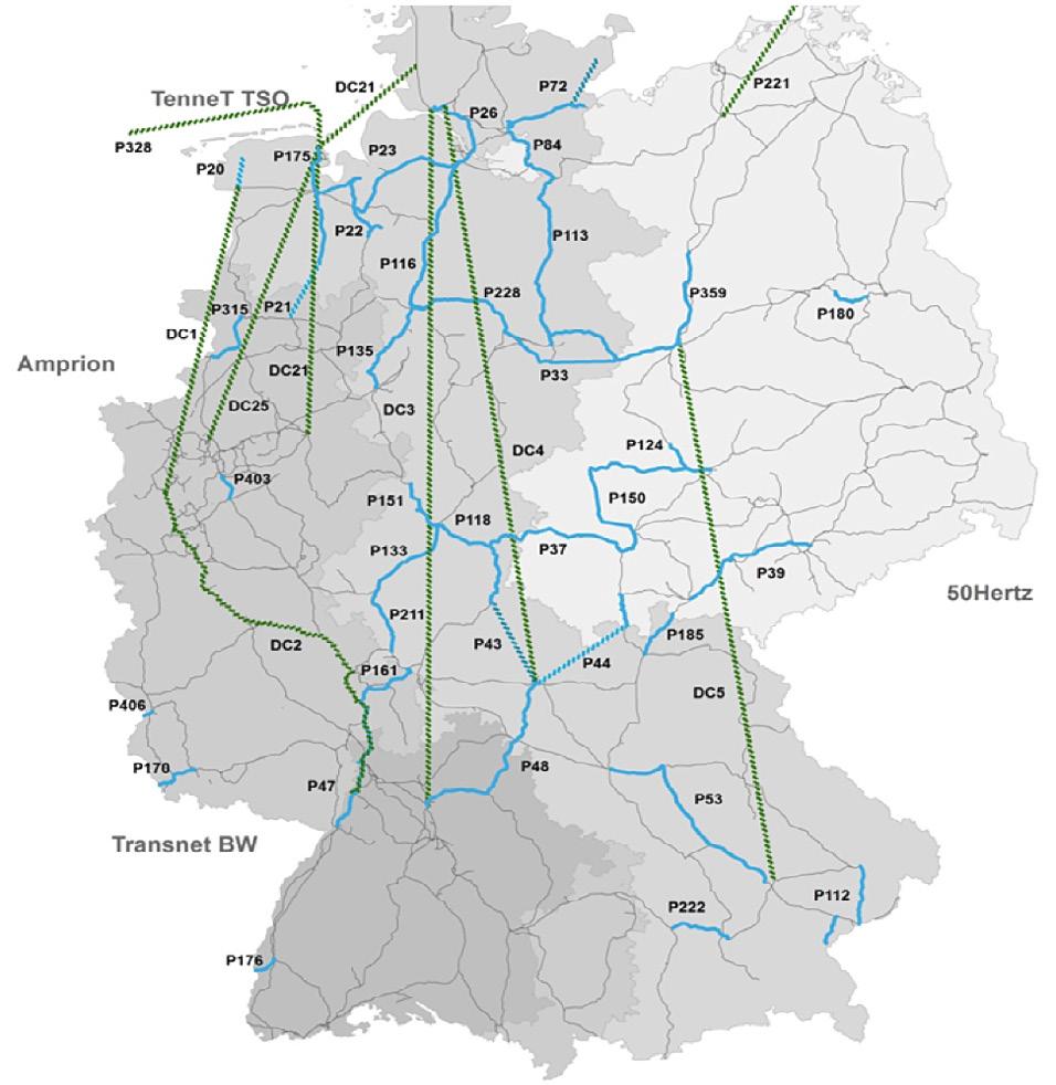
The German grid development is coordinated through a biannual process called “Netzentwicklungsplan” (NEP). Its current version “V2019” targets the trajectory towards 2030 [NEP-1]. The market simulations in this study are based on ‘Scenario B2030’, which is aligned with the TYNDP 2018. It contains further updates, which have been approved by the German regulator (Bundesnetzagentur, BNetzA) since then. These updates are included in the simulations of this study as well 3 Figure 9 displays all confirmed German grid development projects for AC lines (blue) and DC corridors (green) for 2030. The previously outlined trend of significant north to south transmission need can be seen clearly. Bulk RES generation in the north (mainly wind power) needs to be delivered to the main consumption centres in the south. It is important to emphasise the illustrative purpose of that map as further projects might get approved in the near future (c.f. ongoing consultation process for NEP projects wih German regulator BNetzA).

GERMAN HVDC ASSUMPTIONS [FIGURE 10] B1, B2 B1 A1A2 C1 C2 D1 B2 Ultranet SuedLink SuedOstLink Scenarios & Assumptions 3.

Zoom in: German Grid Development Plan (NEP)

STATUS OF APPROVAL FOR GERMAN GRID DEVELOPMENT AS OF JULY 2019 WITH HIGHLIGHTED RES GENERATION AND CONSUMPTION CENTRES [FIGURE 9]

DC line in new corridor AC line strengthening in existing corridor AC line in new corridor Existing grid

To demonstrate the importance of grid expansion to get the renewables in the north of Germany to the consump tion centres in the south, the performed simulations in this study will touch upon a sensitivity that focuses on the importance of the German internal HVDC corridors. The study compares two cases for the HVDC lines. In the reference case, all five corridors in Germany are included in the simulations. For the sensitivity only corridor ‘A Nord’ (A1) and ‘Ultranet’ (A2) are considered in 2030. The network assumptions for Germany are based on “Netzentwicklungsplan (NEP) Scenario B2030 Version 2019”.

AV E LG E M IZEGEM HO R TA ROD E N H U Z E M E RC ATO R C O U RC E LL E S M ON C E A U C H OOZ A U B A N G E V I LL E RO U X AW I R S J U PI LL E S E R A I N G M O U L A N E M EE R H O U T G R A M M E ROMS É E BRUME S OY M A S S E N H OV E N A L EGr O LIXHE M A A SB R AC H T Z A N DV L I E T L L LO VA N E YC K D I L S E N DO E L B R A B OLINT MOG AV E L I N LO N N Y S C HI FF L A N G E D ROG E N B O S B R U EG E L AC H Ê N E G EE R T R U I D E N B E RG B O R S S E L E RILLAND L E VA L BE-DE II G E Z E L L E VA N M A E R L A N T NEMO LINK® Modular Offshore Grid - phase 2 Nouveau corridor Stevin-Avelgem (« Ventilus ») Nouveau Avelgem-Centrumcorridor (« Boucle du Hainaut ») Nautilus (BE-GB II) S T E V I N OVERVIEW OF THE EXTRA HIGH VOLTAGE PROJECTS IN THE PERIOD (2020-2030), EXTRACT FROM THE BELGIAN FEDERAL DEVELOPMENT PLAN 2020-2030 [FIGURE Scenarios11]& Assumptions

There are three major drivers for the Belgium grid expansion needs. First, the stabilisation of the internal grid to be prepared for the nuclear phase-out and a growing decentralised onshore production of wind and solar. Second, the increase of offshore wind production to around 4 GW. Third, the increase in cross-border capacities with all surrounding countries through AC- and DC-connections (e.g. the ALEGrO project).

Zoom in: Belgian Federal Development Plan

In addition to a stepwise strengthening of nearly all major lines, two important new corridors are in the planning: “Ventilus” and “Boucle du Hainaut” (indicated with yellow zones in Figure 11). These new corridors are required to transport the next wave of 2 GW of offshore wind energy (MOG II-project) to the load centres. The Belgian Federal Development Plan [ELI-2] provides more information on these two projects.

Scenarios & Assumptions

Overview on Phase-Shifting Transformers (PST) assumptions

In addition to the grid expansion measures, controllable devices such as Phase-Shifting Transformers (PST) can steer the power flows in the grid up to a certain extent. They can level out the flows in the grid (e.g. redirect flows from lines with high loading to lines with lower loading). As such, they also play a key role in managing the flows in the European electricity system (c.f. Box 1.2).

Figure 12 displays PSTs in the 380 kV grid as included in the simulations for selected countries 4 for 2030. In the performed simulations, PSTs with a significant impact on cross-border flows (blue PSTs in Figure 12) are either optimised before the market or within the market (see Section 3). All PSTs (orange and blue) are subsequently optimised by the TSOs to secure the grid after the market.

The importance of PSTs in the context of the proposed toolbox for higher grid utilisation is further elaborated in Section 5.1.

PSTs INCLUDED IN THE MODEL AND THEIR MAIN PURPOSE [FIGURE 12] (mainly) for internal purpose (mainly) for cross border purpose INT PST XB PST OptimisationMarket ✖ ✓ OptimisationGrid ✓ ✓ Selection for BE, CZ, DE, NL, PL; Not shown: FR, IT, SI. BOX 1.2: PHASE-SHIFTING TRANSFORMER (PST) Power flows in the grid follow the path with the lowest resistance (Kirchhoff’s law), which differs from the com mercial flow of electricity. The power flow in a line is proportional to the difference in phase angle of the volt age between both ends of the line. It can therefore be shifted by controlling the voltage phase angles. A PST is a special form of a transformer, which can steer the power flows up to a certain extent by changing its ‘tap positions’.

4. Namely Belgium, Czech Republic, Germany, Netherlands, Poland. Not shown, but included in the model: PSTs in France, Italy, Slovenia.

Market designmethodologyanalysis 2 2.1. Initial loading calculation 16 2.2. Market clearing simulation 18 2.3. Redispatch quantification 19 2.4. Flow-based market simulations 20

[FIGURE 13]

OVERVIEW

This section details the methodology used in this study for analysing different market designs for 2030. For this, a process with three hourly market simulations has been developed. Figure 13 gives an overview of the different steps in the per formed simulations. First, the transmission capacity avail able for the day-ahead wholesale market is determined by calculating the initial loading of the network elements. In a second step, the day-ahead wholesale market results are calculated. Finally, a model is run to calculate the redispatch needed to secure the grid after the market. For this, a grid model with technical small zones is used (see Section 2.4). The different steps are explained in more detail in the next sections. Section 2.4 provides more information on the mod elling of a flow-based market in this study. Box 2.1 explains some fundamental concepts of the flow-based mechanism. OF THE MARKET DESIGN ANALYSIS METHODOLOGY

Zonal hourly market simulation Grid constraints & loadgeneration/assumptionsforthemodelledzone

106590 75 25 REPRESENTATION

BOX 2.1: FLOW-BASED CONCEPTS

With this GSK, a ‘nodal’ PTDF can be converted into a ‘zonal’ PTDF. The ‘zonal’ PTDF refers to the impact of a commercial exchange between two bidding zones on a certain grid element. This can be easily explained by following example: a commercial exchange of 100 MW would have an impact of 10 MW on a line with a 10% PTDF value (for an exchange between those two bidding zones).

Market design analysis methodology

Zonal hourly market simulation Small zone hourly market simulation

STEP 1 STEP 2 STEP 3

PTDF PTDF stands for Power Transfer Distribution Factor. The nodal PTDFs indicate how energy flows are (unevenly) distributed over the different paths in the network when a power flow occurs between two electrical nodes. An example of such a distribution is shown in Figure 14 for a 100 MW power flow from node A to node D. The distribution given by the PTDFs is determined both by the topology of the grid and the technical characteris tics (impedances) of the grid. PTDFs are calculated for the flows over the grid elements in N state (full network availability) as well as when grid contingencies occur, called the N-1 state (e.g. in the case of a line outage). B C D + 100 MW - 100 MW OF A NODAL SYSTEM AND UNEVEN FLOW DISTRIBUTION [FIGURE 14]

CNEC CNEC stands for ‘Critical Network Element and Con tingency’, a concept used in the flow-based capacity

Determination of the loadinginitialof theelementsnetwork Running of the marketsimulationclearing quantificationRedispatch

GSK GSK stands for ‘Generation Shift Key’, a concept used to model zonal markets. The GSK provides the relative weight of each network node within a bidding zone for a commercial exchange. The GSK translates the change in net position (import/export) of a bidding zone due to a commercial exchange into a change in generation output in the different nodes of the network.

Forcalculation.onecritical network element, different contingen cies (a contingency is sometimes also called N-1 situa tion) can exist for different situations of the network. All relevant critical network elements and respective contingencies compose the PTDF matrix, with rows for each CNEC and columns for each variable impacting the flow on the critical network element.

GSKusing

The developed process for determining the initial loading (i.e. the first step of Figure 13) of network elements is depicted in Figure 16. This process is only used to calculate a best estimate of the initial loading of grid elements. It does not represent a real market clearing.

Remaining Available Margin (RAM) [MW] Initial loading at exchanges0 commercial[MW] Availablecapacity[MW] ILLUSTRATION OF THE INITIAL LOADING OF A NETWORK ELEMENT [FIGURE 15]

2.1.

dispatchusingcalculationscaledandPTDF STEP 1 STEP 2 STEP 3

Market

Zonal hourly market simulation Scaling Flow

PROCESS FOR DETERMINING THE INITIAL LOADING OF

The Remaining available Margin (RAM), being the difference between the available capacity of the line and the initial loading, indicates how much capacity on the grid element can be made available to the market without causing overloads.

NETWORK ELEMENTS [FIGURE 16]

Initial calculationloading

Estimation of the dispatch within bidding zones

design analysis methodology

The first step in the developed methodology calculates the transmission capacity available for the market, by determining the initial loading of the grid elements, i.e. the flow on the grid element in absence of commercial exchanges between bidding zones (e.g. due to internal exchanges within the bidding zone). This is illustrated in Figure 15.

Calculateloadinginitialof all elementsnetworkatno commercialexchanges

First, a zonal market simulation (considering the existing bidding zone configuration) is performed taking into account no initial loading of the grid elements, therefore allowing their full capacity to be used by the market. This allows estimating the dispatch within each bidding zone when commercial exchanges are allowed. In order to determine the initial loading, i.e. the loading in absence of commercial exchanges, the dispatch within each bidding zone is subsequently scaled linearly using its GSK to attain zero commercial exchanges. Using the scaled dispatch (at zero commercial exchanges) within each bidding zone, the initial loading of all network elements can be determined for each hour of the simulated year using the technical small zones PTDF (see later).

Scaling of the dispatch within bidding zone to commercialnoexchanges

Figure 17 explains the process for determining the initial loading of network elements at zero commercial exchan ges. The example uses three nodes A, B and C. Two bidding zones are taken into account: nodes B and C are one bid ding zone (further referred to as bidding zone BC), whereas node A constitutes the other bidding zone. In step 1, it can be seen that a 100 MW commercial exchange occurs from bidding zone BC towards bidding zone A. Within bidding zone BC, node B is exporting 200 MW (100 MW to node C within its bidding zone and 100 MW to node A in another bidding zone).

In step 2, the GSK of bidding zone BC is used to scale the 100 MW commercial exchange. For example, 10% of the 100 MW commercial exchange is compensated on node B (and the remaining 90 MW on node C) resulting in a nodal balance of 190 MW for node B (and -190 MW for node C).

ILLUSTRATION OF THE PROCESS FOR DETERMINING THE INITIAL LOADING OF NETWORK ELEMENTS AT ZERO COMMERCIAL EXCHANGES [FIGURE 17] A C B Commercial exchange -100 MW +100 MW GSK 90%10% A C B Commercial exchange 0 MW 0 MW A C B Commercial exchange 0 MW 0 MW STEP 1 Estimation of the dispatch within bidding zones STEP 2 Scaling of the dispatch within bidding zone to no commercial exchanges STEP 3 Calculate initial loading of all network elements at no commercial exchanges Balance within bidding zone +200 MW -100 MW Scaled balance within bidding zone +190 MW -190 MW Scaled balance within bidding zone +190 MW -190 MW

As bidding zone A consists of only one node, the 100 MW of commercial exchange is compensated entirely on this node. With the resulting scaled balances within the bidding zone, in step 3 flows on network elements can be calculated using the PTDF. These flows, although they result from an exchange within bidding zone BC, are present on all network elements. In Figure 17, the initial loadings are represented with the green arrows.

Market design analysis methodology

Virtualprovidedcapacity[MW]Availablecapacity[MW]

Market design analysis methodology

y Grid constraints: the flow-based market mechanism only considers a subset of the grid constraints. In general only grid constraints that are relevant for cross-border exchanges (for example having a PTDF value above an agreed threshold) are taken into account. In other cases only the cross-border grid elements are considered as constraints for the model.

Optimisation of PSTs and (internal) HVDCs in the market clearing: in some of the performed simulations in this study, the set points of PSTs and internal HVDCs are optimised in the market clearing. Further explanations can be found in Box 3.2.

ILLUSTRATION OF THE INITIAL LOADING OF GRID ELEMENTS AND THE APPLICATION OF MINIMUM MARGINS ( min RAM) [FIGURE 18]

Market clearing simulation2.2.

In this step, the zonal market clearing is simulated by an hourly market simulation in the Antares software. This market clearing simulation mimicks the day-ahead market coupling that is in place today in Europe.

The initial loading of the network elements, i.e. at zero commercial exchanges, calculated in the previous step (see Section 2.1), is taken into account here. The difference between the available capacity of the network element and the initial loading defines the capacity that is available for the market (RAM). Network elements can be (almost) fully congested by their initial loading, leaving little to no capacity available for the market. In such a case, a minimum margin (minRAM) for the market can be imposed on the network element. Such minimum margins can result in higher overloads after market clearing, as they provide ‘virtual’ transmission capacity to the market, masking the underlying grid constraints. The process of applying minimum margins is illustrated in Figure 18. No application of minRAM Application of minRAM Remaining Available Margin (RAM) [MW] Initial loading at exchanges0 commercial[MW] Availablecapacity[MW] Remaining Available Margin (minRAM) [MW] Initial loading at 0 exchangescommercial[MW]

Other important inputs for the market clearing simulations in this study are:

Section 3 provides more information on the assumptions taken for the different simulated market models for 2030.

The market clearing simulation mimics the European dayahead market clearing, by determining the net positions of the bidding zones in a way that maximises welfare while respecting the considered grid constraints. It defines the market dispatch within each bidding zone and the according electricity market price for that bidding zone.

The simulations in this study are based on a national cost-optimised redispatch strategy for the quantification of the redispatch volumes and costs. Cross-border redispatch is only considered where absolutely necessary (i.e. crossborder redispatch has a penalty cost in the optimisation). This could lead to an overestimation of the redispatch costs and volumes since cross-border redispatch, when properly coordinated, would reduce costs and volumes.

On the other hand, in the simulations all flexible generation and demand can be redispatched within the bidding zone, without add-ons to the marginal cost and without RES subsidy compensation, which represents an underestimation of the costs and volumes. Therefore the applied redispatch scheme is assumed to give overall representative results.

In order to assess the performance of a market design in terms of welfare creation, it is important to also take into account the costs to solve potential overloads that are present in the grid after the market clearing. To quantify those costs, a third hourly market simulation is performed with the Antares software, taking into account all the grid elements of the model (whereas in the market clearing simulation only a selection of the grid elements is taken into account as explained before).

Market design analysis methodology

All controllable devices (PST & HVDC) can be fully used to secure the grid in this third simulation step.

The hourly market dispatch result of the zonal market clearing step from Section 2.2 could result in flows on network elements which are higher than their available capacity. In this case, the TSO will intervene after the market in order to secure the grid, i.e. making sure that flows will stay within operational limits. The main reasons why the market dispatch might lead to overloads are:

Redispatch quantiﬁcation

First the dispatch, resulting from the market clearing simulation in step 2, is calculated for each of the technical small zones (see Section 2.4 for more explanations on the technical small zones). The flows on all grid elements are then calculated on the basis of the technical small zone PTDFs.

This study considers that all redispatch is based on marginal costs (i.e. no ‘add-on’ is considered when calculating redispatch costs). Curtailment of renewables, like wind, is considered at zero marginal cost in this study (i.e. not accounting for potential opportunity losses resulting from subsidy mechanisms).

2.3.

y Inaccuracies in modelling the loading of grid elements (amongst others due to the use of a GSK); y Application of virtual margins (minRAM); and y Consideration of only part of the grid elements as constraints for the market.

The loading of the grid elements is now defined on the basis of the more accurate technical small zones dispatch resulting from the market (instead of a dispatch simulated with a zonal GSK). This step can show that grid constraints are violated. In this third market simulation, the dispatch in the technical small zones is allowed to deviate from the dispatch (defined by the market clearing in step 2) in order to achieve a dispatch which respects all grid constraints.

By calculating how much the technical small zone dispatch has to change compared to the market clearing simulation from step 2, one can define the redispatch volume (including volumes of renewables that are curtailed). Moreover, the additional costs associated with these changes, moving away from the zonal market solution, provide the simulated redispatch costs.

The hourly market simulations in this study have been performed with the Antares simulation software. Antares was at the basis of various other studies performed by Elia and other TSOs (for example the ‘Elia Adequacy & Flexibility study for Belgium 2020-2030’ [ELI-1]). More information on the simulation tool can be found in [ANT-1]. The next paragraphs provide an overview of specific assumptions in the simulation model for this study.

Flow-based market simulations

The current day-ahead wholesale electricity market in Europe takes network constraints into account as a mix of flow-based constraints and NTC constraints. Today, the day-ahead flow-based Capacity Calculation Region (CCR) (of which Belgium is part) is limited to the CWE countries: Belgium, the Netherlands, France, Germany, Austria and Luxemburg. In the context of this study, also the following market areas are modelled using flow-based constraints: Poland, Czech Republic, Slovenia, Italy North and Switzerland. Figure 19 summarises the simulated perimeter and the way network constraints are taken into account in this study. Exchanges between the NTC modelled area and the flow-based modelled area are in this study handled through advanced hybrid coupling with a fixed maximal exchange capacity. hybrid coupling for exchanges between NTC and FB modelledFlowzoneBased modelled

NTCAdvanced

Not

SIMULATED PERIMETER IN STUDY [FIGURE 19] Market design analysis methodology

2.4.

admissiblephysicallyexchanges underInterconnectorsconsideration A C [MW] A C [MW] A B [MW] A B [MW] NTC domain

Flow-based The flow-based method (FB) considers transmission capacity constraints for commercial exchanges between different market areas by considering the physical limits of every relevant critical network element (CNE) of the grid. The domain of possible commercial exchanges for market coupling is thus not limited by a generalisa tion of exports viewed per border individually (i.e. NTC approach), but rather by a set of constraints (FB con straints) considering the level of congestions on the critical network elements (CNEs) under normal (N) and grid contingency (N-1) situations (CNECs). Different commercial exchanges cause different physical flows on considered CNEs in the grid. Therefore, in the FB approach commercial exchanges on different borders are not independent from each other. In the flow-based mechanism the impact of cross-border exchanges on the grid is modelled more accurately. This approach is illustrated in Figure 20 on the right.

COMPARISON

NTC NTCs are calculated by TSOs per border between bid ding zones and provide the commercial exchange cap acity that can be allocated by the market. TSOs of neigh bouring market areas coordinate bilaterally to align the NTC values on their common borders, which results in the NTC solution margin. In a NTC simulation approach, each border (interconnector) is treated independently from other borders. This approach is illustrated in Figure 20 on the left.

21 BOX 2.2: FLOW-BASED VERSUS NET TRANSFER CAPACITY (NTC)

[FIGURE 20] Range

-400-2004002000 Net Transfer capacity calculation Flow-based calculation -400-2004002000 FB domain

‘Flow-based’ (FB) is a method for capacity calculation and allocation which accurately models the impact of commercial exchanges on the modelled grid elements (impedances, physical capacities). This opposed to the so-called ‘Net Transfer Capacity’ (NTC) approach, which assumes only one commercial capacity between two market zones (for each direction). In both the flow-based and the NTC market design, system operational security constraints are respected, fulfilling the N-1 criteria.

Grid

The NTC method is applied in this study for the blue region in Figure 19. The red zone is modelled through a flow-based method. Commercial exchanges between the blue and the red zone in Figure 19 are modelled through Advanced Hybrid Coupling (AHC). Regulation EU 2015/1222 on Capacity Allocation and Congestion Management (CACM) sets the flow-based method as the target model for Europe. nodes and critical network elements under considerationconstraintFlow-based -400 -200 0 200 400 OF NTC APPROACH (LEFT) AND FB METHODOLOGY (RIGHT) of -400 -200 0 200 400

Market design analysis methodology

When zonal market designs are simulated, the technical small zones are merged into the existing bidding zones. This merging is done using ‘Generation Shift Keys’ (GSKs), indicating how commercial exchanges will be divided among each technical small zone within the bidding zone. In this study, the GSKs are calculated as the fraction of dis patchable thermal capacity present in the technical small zone as a part of the total dispatchable thermal capacity in the whole bidding zone concerned.

The technical small zones are considered as copper plates in the modelling, meaning that there is no grid (and hence no congestions) modelled within those zones. Given the high resolution of the model (small size of the zones), this is a realistic assumption when modelling congestion management in the pan-European electricity markets.

The PTDF matrix used throughout this study takes into account up to six of the most constraining contingencies for each critical network element. Only 380 kV critical net work elements are taken into account as they are most rel evant for transporting the bulk power flows resulting from pan-European electricity markets. For one of the analysed market designs (Flex-In-Market design, see Section 3.3), the concept of ‘important’ internal (within one bidding zone) network elements is used. Without taking any prejudice on the optimal or final criterion, this study assumed that lines with a PTDF threshold above 10% for commercial exchanges are considered as ‘important’ internal network elements5.

TECHNICAL SMALL ZONES USED FOR FLOW-BASED MODELLING [FIGURE 21]

Market design analysis methodology

5. In the CWE flow-based mechanism this threshold is currently defined as 5%.

In order to correctly determine flows on network elements within the flow-based modelled zone, technical small zones are defined and the assumed generation and load in the model are divided over these different technical small zones (see Figure 21). For most countries, the small zones are those used within the context of the ENTSO-E TYNDP 2018 Flow-Based methodology [ENT-1]. However, for this study the Belgian and German bidding zone have been modelled with more small zones in order to increase the accuracy of the modelled power flows: y Belgium is modelled using three small zones (East –Center – West); y Germany is modelled using 21 small zones, as often done in German grid development studies.

Analysed market designs 3 3.1. Small zones design as technical reference 25 3.2. Reference market design 26 3.3. Flex-In-Market design 27

The full details of the studied designs are summarised in Table 3. More in-depth explanations are provided in the following sections.

This section provides more details on the analysed market designs in this study. The focus of this study is on the reference market design and Flex-In-Market design. The technical small zones design is only simulated as a technical reference and for redispatch calculation.

The main characteristics of the different market designs are as follows.

Technical small zones design: this design, based on very small technical bidding zones, is simulated only as technical reference and is mainly used for redis patch quantification (see Section 2.3). All 380 kV grid elements are taken into account for the market clear ing, and no virtual margins (minRAM) are applied on them. The set points of PSTs and internal HVDCs are optimised in the market clearing.

TABLE 3: ANALYSED MARKET DESIGN OVERVIEW BIDDING CONFIGURATIONZONE ELEMENTSINTERNAL minRAM PST & HVDC IN MARKET DISPATCHHUBS Technical small zones design smallTechnicalzones N/A* 0% ✓ ✖ Reference market design Existing None 70% ✖ ✖ Flex-In-Market design Existing Important ones (>10% PTDF) 0% ✓ ✓ *As for the small zone technical reference design all modelled grid elements are crossing bidding zone borders, these are taken into account by default.

y Flex-In-Market design: as for the reference market design, the existing bidding zone configuration is kept. However, selected important internal grid elements (see Section 2.4) are taken into account in addition to the cross-border elements. There is no application of minimum available capacities (minRAM). Contrary to the reference market design, the market clearing can optimise extra flexibility directly within the algorithm (in the form of set points of PSTs, (internal) HVDCs and Dispatch Hubs). This is explained further in this section.

24 Market designs analysed

Reference market design: this design reflects the currently foreseen way of implementing the policies for 2030. The model uses the existing bidding zone con figuration. The market clearing simulation considers only cross-border grid elements and a minRAM of 70% is provided on them in accordance with the requirements of the CEP. Set points of controllable devices such as PSTs and HVDCs are optimised by the TSOs before the market clearing.

As a result of those assumptions, no overloads will be observed after market clearing. Therefore this market design is used as a basis for the redispatch quantification in this study (cf. Section 2.3). THE “SMALL ZONES” USED IN THIS

Small zones design reference designs

STUDY [FIGURE 22]

This technical reference simulates each small zone as a separate bidding zone that is considered as a copper plate (c.f. Section 2.4). Therefore, there is no initial loading at zero commercial exchanges (see Section 2.1) on the grid elements. All transmission capacity between the small zones is made available to the market. The technical small zones model gives the market clearing more degrees of freedom to calculate the optimal market dispatch, leading to a dispatch with higher welfare. However, other effects such as reduced market liquidity, reduced portfolio bidding are not considered in this study. Therefore the welfare results need to be interpreted with caution. Given the copper plate assumption, this market design does not consider any congestions within the small zones. All modelled grid constraints are considered in the market clearing.

as technical

analysed

EXAMPLE OF

3.1. Market

As discussed in Section 2.4, the Antares simulation model functions with technical zones which are smaller than the existing bidding zones (see Figure 21 for an example). In this study, the technical small zones design is not proposed as a market design. The model is only used for quantifying redispatch and to see where the market dispatch of the small zones design deviates from the dispatch from the reference market design (see Section 3.3). In this design, all controllable elements (PSTs & HVDCs) are available for optimisation in the market clearing.

Only cross-border grid elements are considered as constraints during the market clearing. The reference market design leads to potentially high overloads in the grid after the market, which the TSOs then resolve by changing grid topology, changing PST and HVDC set points or by activating redispatch after the market clearing (step 2 in Figure 23).

Market designs analysed

welfare

Reference market design

High redispatch overloads with flexibility after market Challenge locational information of bids in bidding overall

behind 1 12 2[MW]capacityAvailable[MW]MarginVirtual REFERENCE MARKET DESIGN OVERVIEW [FIGURE 23]

The reference market design reflects the currently foreseen implementation of the policies for 2030. It is based on the existing bidding zone configuration with bidding zones largely coinciding with Member States borders. Only grid elements crossing bidding zone borders (also referred to as cross-border grid elements) are considered as grid constraints (CNECs) in the market clearing, as specified in the ACER decision on the CORE CCM [ACR-1]. In line with the ‘Clean Energy Package’ regulation [EUC-3], a minimum of 70% of the available capacity of each grid element is made available to the market (via the minRAM mechanism as explained in Section 2.2). As explained before, the application of the minRAM scheme and ommittence of internal lines can result in grid overloads after the market (in case virtual transmission capacity is provided to the market).

In the reference market design, PSTs are not optimised in the market clearing. The blue PSTs in Figure 12 are located close to the borders, are optimised by TSOs two days before the market clearing to maximise transmission capacity in the direction of the estimated market clearing. In the methodology described in Section 2, this is done in the first step: initial loading calculation. The taps of the blue PSTs are subsequently considered to be fixed during the market clearing simulation. The blue PSTs therefore do not add degrees of freedom to the market clearing. This type of modelling, in which a fraction of the PST capacity is used to optimise capacities before the market clearing, is comparable to current operational practice. All of the PSTs (orange and blue in Figure 12) are optimised by the TSOs to solve overloads after the market clearing when securing the Figuregrid.23 schematically shows the principles and the challenges of the reference market design. This market design relies on the application of minimum margins (minRAM) in order to provide 70% of the available capacity of the grid element for cross-zonal trade as required by the Clean Energy Package [EUC-3]. This leads to providing virtual capacities to the market in case the initial loading exceeds 30% of the available capacity of the grid element (step 1 in Figure 23).

initial

volumes …TSO solves

zone Lower

70% No

Initial loading increases as result of energy transition and grid lagging

Reference market design3.2.

Virtual margin provided to market… loading

Reference market design Market has not a good view on the grid. Flexibility to secure the grid is therefore optimised after the market. Flex-In-Market design Market needs accurate information on grid constraints as flexibility to solve congestions is optimised within the market.

The variables which can be used to achieve this optimal dispatch, also referred to as ‘degrees of freedom’, are classically the bidding zone balances (i.e. net position of import or export). However, the electricity system has a vast multitude of degrees of freedom. Today a large part of those degrees of freedom are optimised after the market clearing (e.g. redispatch on generation or demand units). Also controllable devices such as PSTs and (internal) HVDCs can bring additional degrees of freedom. The concept of degrees of freedom is illustrated in Figure 24. In the reference market design the TSOs provide minimum available margins to the market and only consider cross-border grid elements as constraints for the market clearing. This inevitably leads to overloads in the grid. In a later step, TSOs then solve those overloads by changing grid topology, set points of PSTs and (internal) HVDCs and by performing redispatch. In contrast, the Flex-In-Market design aims to optimise most of those flexibilities directly within the market clearing. It is therefore important that the market clearing has a good view on the real grid constraints. If not, those flexible resources would be optimised and activated on the basis of inaccurate information, leading to a sub-optimal solution. Moreover, those means might not be available anymore (as they are already used) to solve then the real overloads after the market clearing. This is explained in Figure 25.

Flex-In-Market design3.3.

Market designs analysed

The pan-European day-ahead wholesale electricity market tries to find an optimal dispatch in the sense that it looks for the solution with the minimal system cost, taking into account grid constraints (flow-based or NTC constraints).

Zone B Zone A Zone C SCHEMATIC ILLUSTRATION OF THE RANGE OF DEGREES OF FREEDOM WHICH CAN BE MADE AVAILABLE TO THE MARKET [FIGURE 24] LoadGenerator

This study proposes an improved Flex-In-Market design that provides additional flexibility to the market clearing for efficiently managing congestions within the market instead of after the market. In this context ‘flexibility’ refers to the degrees of freedom available to the market clearing under the form of PSTs, HVDCs and Dispatch Hubs (see the Technical Summary of this study reference [ELI-5] for a detailed description of the concept of Dispatch Hubs).

ILLUSTRATION ON THE NEED FOR BETTER INFORMATION ON THE GRID FOR THE MARKET WHEN ADDITIONAL FLEXIBILITY IS PROVIDED IN THE MARKET [FIGURE 25] Need to bettermarketprovidewithinformationonthegrid

zones

The Flex-In-Market design optimises the flexibility from PSTs, (internal) HVDCs and so-called Dispatch Hubs directly in the market clearing. This means that instead of having TSOs to estimate the optimal set points of PSTs and internal HVDCs before the market clearing, it is now the market clearing that indicates the most optimal settings of those devices from a welfare point of view. Concretely the market clearing now has the flexibility to change the set points of those devices to direct flows from a congested grid element towards grid elements on which capacity is still available (i.e. redirecting flows). In this way, the total commercial exchange between bidding zones can be increased, thus allowing for a more optimal dis patch (e.g. by reducing loop flows,…). In the Flex-In-Market design, the TSOs operate PSTs and HVDCs and are respon sible for defining the final settings of those devices when securing the grid after the market. Figure 26 gives an over view of the PSTs, HVDCs and Dispatch Hubs that are opti mised in the performed simulations on the Flex-In-Market design. Besides the additional flexibility which can be introduced in the market by PSTs and (internal) HVDCs, from Figure 24 it is clear that also other resources, such as conventional generators, can provide extra degrees of freedom to the market. By selecting specific resources (e.g. conventional generation or redispatch potential) which have a high impact on congested grid elements (e.g. located on both sides of a grid element that often restricts the market), additional degrees of freedom can be offered to the market clearing for managing congestions, while keeping the existing bidding zones untouched. This is the under lying idea behind the concept of Dispatch Hubs (see the Technical Summary of this study reference [ELI-5] for a detailed description of the concept of Dispatch Hubs). HVDC FLEX-IN-MARKET 1a: Perform a technical small simulation the 1b: Compare the absolute deviation of net positions of the small for on hourly basis (abso lute Clusters with the highest differences (a threshold of 2 TWh on a yearly basis was used) net position were considered as good locations for Define on an hourly basis the 90th percentile of the absolute deviations in net positions for that This defines the capacity of the Dispatch Hub volume which allows to cover most of the

zone.

DESIGN [FIGURE 26] 1.31.3 0.9 0.9 1.1 0.8 0.9 1.4 1.2 4.0 1.3 1.7 0.81.2 ++ HubsDispatch[GW]B1 A1A2 C1 C2 D1 B2 In this study two potential ways for defining the location and size of Dispatch Hubs are identified. In the performed simulations, a methodological approach has been fol lowed, as illustrated on the left in Figure 27. The process consists of following steps: y Step

reference market simulation (Section 3.2); y Step

The following aspects are important to provide the market an accurate view on the grid: Provide the most relevant ‘important’ grid constraints with respect to cross-zonal exchanges to the market; y Provide a high quality estimation of the initial loading on the grid elements (i.e. with no commercial exchan ges) to the market; and y Incorporate an accurate model for simulating the flow impact of cross-zonal exchanges on a specific trans mission line.

values).

deviations. Market designs analysed

The proposed Flex-In-Market design incorporates selected important internal grid elements. This study, without any prejudice to the final criterion, considers grid elements on which at least 10% of at least one commercial exchange between any combination of two bidding zones (see Sec tion 2.4) passes. In addition, no minimum margin (minRAM) is made available on grid elements at zero commercial exchange. This ensures that the correct information is avail able to the market in order to manage the congestions in the most efficient way in the market clearing.

2 Dispatch Hubs 3 FLEXIBILITY OPTIMISED IN THE MARKET COUPLING IN THE

PST 1

both runs

Dispatch Hubs; •

zones

(Section 3.1) and

•

Other procedures to determine size and location of Dispatch Hubs can be envisioned. The optimal location of the Dispatch Hubs strongly depends on the underlying congestions in the grid. Their location must be defined by the TSOs in a transparent way. As illustrated on the right in Figure 27, Dispatch Hubs could also be introduced at both sides of a structural congestion. The size of the Dispatch Hubs could then be determined based on the size of the overloads that must be resolved. ALTERNATIVE Location and size of Dispatch Hubs Dispatch Hubs at opposite sides of a congestion Dispatch Hubs are located at opposite sides of a structural congestion Size of Dispatch Hub is defined by the size of the congestion to be resolved Location: select the technical small zones with largest absolute deviation Size: define X% percentile of hourly deviations the Dispatch Hub must cover • Run a model with existing bidding zones and technical small zones Calculate the difference in net position for each technical small zone for each hour For each hour of the year Congestion

The result of the previously described process (left of Figure 27) is shown in Figure 28. The figure shows the Dispatch Hub capacity and location for the 14 Dispatch Hubs which are used in this study. In the performed simulations, the Dispatch Hubs consist of large conventional thermal production units, except for the 4.0 GW in the north of Germany. In this specific zone, a small fraction of the wind of the zone has been isolated in the Dispatch Hub (in absence of other means to manage congestions in the applied 2030 model). Dispatch Hubs are introduced as a new concept in this study. The concept requires further discussion and elaboration with different stakeholders on European level. USED FOR THIS STUDY

[GW] [FIGURE 28] 1.31.3 0.9 0.9 1.1 0.8 0.9 1.4 1.2 4.0 1.3 1.7 0.8 1.2 Market designs analysed

2 •

•

PROCESS FOLLOWED IN THIS STUDY TO DETERMINE THE LOCATION AND SIZE OF THE DISPATCH HUBS (LEFT) AS WELL AS A POSSIBLE

or + -

DISPATCH HUB CAPACITY AS

PROCESS (RIGHT) [FIGURE 27] marketSimulatedispatch 1a

•

on the grid In market After market 1 + Solve residual (small) congestions efﬁciently3 + € PRINCIPLES OF THE FLEX-IN-MARKET DESIGN [FIGURE 29] Coordinated cost basedschemeredispatch Include minimumNogridimportantmostinternalelements(virtual) capacity DispatchHubs ~ = Optimise in market: PST HVDC(XB)(internal) Topological Actions and

Toolbox

Figure 29 summarises the principles of the analysed FlexIn-Market design. First, the market is provided with a better view on the grid constraints, by removing virtual margins and including important internal grid elements as constraints in the market clearing. Next, the market clearing gets access to more flexibility to manage congestions in a more efficient way, under the form of PSTs, internal HVDCs and Dispatch Hubs. This allows a higher utilisation of the grid and reduces the overloads after the market clearing. (small) congestions will still need to be solved after market clearing, and for this an optimal coordinated costoptimised redispatch scheme should be implemented.

Residual

30 Market designs analysed

The goal of the Flex-In-Market design is to provide a larger flow-based domain compared to the reference market design. Solutions can be envisaged to mitigate situations where insufficient flexibility would be offered to the market to provide a domain that at least matches the reference market flow-based domain. Those measures were not considered in this study. with view

efﬁcient measures to manage congestion2Give market a better

PTDF MATRIX FOR EVOLVED FLOWBASED MODELLING OF PSTs, HVDCs AND DISPATCH HUBS [FIGURE 31] BE NL DE FR PST 1 HVDC DH BE CNEC 1 CNEC 2 CNEC 3 CNEC MarketX designs analysed

In the Flex-In-Market design, the TSOs will provide in a first stage technical information regarding the control lable devices to the market algorithm. This technical information includes the range of set points that is available for the market, as well as the flow impact of changing the set points of these controllable devices on the considered grid elements in the market. This information is introduced as new variables (degrees of freedom) in the flow-based model. For both the PSTs and HVDCs, these additional variables correspond to additional columns in the PTDF matrix, as shown in Figure 31. As explained in Box 2.1, the PTDF matrix has a row for each CNEC and a column for each variable impacting the flow on the critical network element. On top of the net positions of the bidding zones, columns are also added for the set points of the PSTs and HVDCs.

For the optimisation of both HVDCs and PSTs in the market clearing, the Flex-In-Market design uses the con cept of evolved flow-based. Evolved flow-based allows the market clearing algorithm to define optimal set points for these controllable devices, in order to deter mine a dispatch which generates the highest welfare. In today’s market design, the set points of PSTs and HVDCs are optimised by TSOs before the market to provide as much transmission capacity as possible in the direction of the estimated market outcome. Their set points cannot be changed by the market clearing algorithm subsequently. The differences between the Flex-In-Mar ket design and the reference market design are shown in Figure 30. On the left, only the net positions of the bidding zones are taken into account as variables in the market clearing algorithm, whilst on the right additional variables are added to the market optimisation.

The Flex-In-Market model additionally considers PSTs, HVDCs & DHs CNEC cross borderHVDCPST Dispatch DispatchinternalHubPSTHub

CLEARING

The current market model considers only Bidding Zones cross borderInternalline CNEC CNEC

EXAMPLE

31 BOX 3.1: OPTIMISATION OF HVDC s , PSTs AND DISPATCH HUBS WITHIN THE MARKET

OPTIMISATION OF PSTs, HVDCs AND DISPATCH HUBS THROUGH EVOLVED FLOW-BASED MECHANISM [FIGURE 30]

The Flex-In-Market design defines optimal set points for the controllable devices in the market. Afterwards the TSO will define the final set point of those devices when securing the grid. The TSOs then apply the final set point on the controllable devices they operate. Additional degrees of freedom can also be created by the inclusion of Dispatch Hubs. In the market clear ing, Dispatch Hubs are flexible resources or redispatch potential that can be optimised independently from the bidding zone in which they are located. Depending on the implementation, separate market bids are provided for each individual Dispatch Hub. The impact of a change in net position of a Dispatch Hub on each CNEC is calculated and included in the PTDF matrix. A change in net position in a Dispatch Hub impacts the network constraints in the same way as the other vari ables represented by the columns of the PTDF matrix (see Figure 31), and no additional constraints are added when Dispatch Hubs are used. This network impact is taken into account by the market algorithm to define the net position and price within the Dispatch Hub (via the flow-based mechanism). OF A

In the market bids variant of Dispatch Hubs, market par ties have to submit separate bids for resources included in the Dispatch Hubs (e.g. conventional generation units). In this case, TSOs need to submit the relevant information of the Dispatch Hub for the PTDF matrix to the market. The market clearing will then directly optimise the resources included in the Dispatch Hubs (instead of selecting redispatch potential for activation).

THE VARIANTS OF DISPATCH HUB IMPLEMENTATION [FIGURE 32] ‘Redispatch potential bids’ variant ‘Market bids’ variant DH bids RD potential Bids in DH Market Results Market results for DHRD order SettlementFinancial SettlementFinancial € € Information on DH (effect on grid, etc.) Information on DH (effect on grid, etc.) Market designs analysed

(NominatedNEMOs electricity operator)market (NominatedNEMOs electricity operator)market MarketParties MarketParties

In the redispatch potential bid variant, a Dispatch Hub represents the redispatch potential, at a certain volume and a certain price that is available at a specific location in the grid (sell or buy bids). Before the market clear ing, TSOs submit ‘Dispatch Hub (DH) bids’, as well as the impact of the Dispatch Hubs on the grid elements (extra column in the PTDF matrix). These bids are then included in the market clearing in the same way as other bids. If the market clearing selects ‘DH bids’, the TSO needs to activate (after the market clearing) the under lying redispatch potential. This approach would allow for a wait and see approach, as TSOs could further wait and see whether the RD potential must be activated, which could be interesting in case of redispatch poten tial on renewables, meaning that the TSO could wait until a later moment on the need for RES curtailment.

This study identifies two distinct variants of Dispatch Hubs (see Figure 32). Dispatch Hubs can contain redis patch potential bids (left of the figure) or market bids (right of the figure). The main difference between both methods is whether Dispatch Hubs contain physical assets (e.g. conventional generation) or the redispatch potential of those assets. The mechanics for optimising Dispatch Hubs in the market, as explained in Box 3.1, are similar for both methods.

In the redispatch potential bids model, the market first settles the selected redispatch potential with the TSO. Afterwards the TSO settles the called upon redispatch with the market parties.

All simulations performed in this study are based on this Bothapproach.variants of Dispatch Hubs have advantages and disadvantages. Further discussions are needed on Euro pean level with other TSOs, market parties and policy makers on the possible variants of Dispatch Hubs. TSOs TSOs

32 BOX 3.2: TWO WAYS FOR IMPLEMENTING DISPATCH HUBS

Result33 analysis 4 4.1. How to understand the results? 34 4.2. Simulation results for reference market design 35 4.3. Role of grid infrastructure in the next stage of the energy transition 39 4.4. Simulation results for Flex-In-Market design 41

It is important to highlight some differences in the performed simulations compared with previous studies by Elia and/or 50Hertz. Given the purpose of the performed simulations (i.e. to quantify relative differences between scenarios), these differences are assumed to have no significant impact on the conclusions of the study. The differences are listed below: No detailed modelling of Power to Heat or Power to Gas, as is performed in the German Federal Grid Development Plan [NEP-1]; No modelling of Vehicle to Grid technology; Modelling of demand side response at €400/MWh for all considered countries and with one type of temporal constraints; and No limit on the maximal import or export for any bidding zones.

 All simulations assume perfect foresight, e.g. not accounting for forecast errors of intermittent renewable production.

Result analysis

The simulations in this study assess the impact of changes in grid infrastructure or market design in the European interconnected electricity system on the generated welfare. The study focuses on relative effects caused by those changes and their order of magnitude. Further discussion and elaboration with various stakeholders on the proposed concepts is required.



The market simulations in this study are performed with the software tool Antares [ANT-1]. The Antares tool simulates the European electricity market on an hourly basis with following underlying assumptions:

How to understand the results?

 Generators bid at short-run marginal costs, not taking into account eventual extra costs to recover investments; The market clearing assumes perfect market conditions, and does not take into account portfolio optimising strategies or market power; and

4.1.

The market simulations are performed for an entire year (8760 hours), representing the meteorological conditions of 2012. As this study focuses on orders of magnitudes and relative comparisons between different options, the insights obtained on that basis can be considered relevant and robust.



YEARLY PRODUCTION MIX AFTER MARKET CLEARING FOR THE REFERENCE MARKET DESIGN IN 2030 [FIGURE 33]

4.2.1. Simulation results for reference market design

Figure 33 shows the simulated yearly production mix (i.e. the energy produced per technology) for the reference market design after market clearing (before securing the grid, i.e. not taking into account changes due to redispatch). The results are aggregated per country on the left side of the figure. The detailed production mix on technical small zone level is shown on right side for a selected region. The size of the circles on the right side is proportional with the volume of produced energy within the small region. Figure 33 provides general insights on the resulting generation mix for the performed 2030 simulations. For example, while the technical small zones in the north of Germany are characterised by high onshore and offshore wind generation, the southern small zones have more photovoltaic generation.

Simulation results for reference market design4.2.

In this section, the simulation results for the reference market design, as described in Section 3.2, are shown. First, some general simulation outcomes are provided in Section 4.2.1. Next, Section 4.2.2 highlights the differences in market dispatch between the technical small zones and the reference market design. These results are used to defi ne the location and size of Dispatch Hubs for the FlexIn-Market design (cf. Section 4.3).

HYDROSOLARWINDOTHERGASCOALNUCLEAR

Result analysis

Figure 34 shows the yearly balances (i.e. net position in TWh for the simulated year 2030) for the reference market design after market clearing and before redispatch. It shows a significant positive balance for the northern part of Germany (coastline North Sea and Baltic Sea), resulting from high wind generation (see Figure 33). Consumption centres are located more in the south of Germany (nega tive balance). Therefore, the power produced in the north of Germany has to be transported towards the consump tion centres (e.g. in south of Germany or neighbouring countries). France and Norway are net exporters of energy in the performed simulations.

YEARLY NET BALANCES AFTER MARKET CLEARING FOR THE REFERENCE MARKET DESIGN IN 2030 [FIGUREBalance34] [TWh/y] -100 – -50 -50 – 0 0 – 50 50 – 100 Result analysis

The balances shown in Figure 34 do not represent the final physical dispatch, since redispatch needed to secure the grid is not included. Figure 36 shows the simulated redis patch volumes in TWh for each of the technical small zones for the reference market design. In Germany, it reveals a need for downward redispatch in the north of Germany (mainly federal states of Schleswig-Holstein and Lower Saxony) and for upward redispatch in the south and west of Germany (mainly federal states of North Rhine-West phalia, Hesse, Baden-Wuerttemberg, Bavaria).

An analysis was performed on the impact of high and low wind conditions in Germany on the European interconnected electricity system. Different situations were defined: values for high (low) wind conditions represent the average value for all hours where more (less) than 67% (33%) of the yearly maximum observed wind infeed 6 is realised in Germany. Figure 35 shows the resulting average balance of the technical small zones as defined in the market clearing (i.e. before securing the grid with a.o. redispatch) for the two situations defined above. The color scale flows from dark green (high export), to dark red (high import). The left of Figure 35 illustrates the ‘low wind’ situation and the right part of the figure the ‘high wind’ situation.

NET AVERAGE POWER BALANCE IN [GW] OF DIFFERENT GEOGRAPHICAL AREAS FOR LOW (LEFT) AND HIGH (RIGHT) WIND CONDITIONS IN GERMANY [FIGURE 35] Average balance [GW] -15 – -10 -10 – -5 -5 – -2 -2 – 0 0 – 2 2 – 5 5 – 10 10 – 15 Around 40 GW to transportedbefromthenorthofGermany High wind conditions in Germany Average balance [GW] -15 – -10 -10 – -5 -5 – -2 -2 – 0 0 – 2 2 – 5 5 – 10 10 – 15 Low wind conditions in Germany 6. For the 2030 simulation, on the basis of 2012 meteorological conditions.

37 Result analysis BOX 4.1: LOW AND HIGH WIND CONDITIONS IN GERMANY

In the ‘high wind’ situation, the north of Germany, with high offshore and onshore wind production capacity, is exporting significant volumes of wind energy. This energy is flowing to the consumption centres in the south of Germany and is exported to neighbouring countries. The export in the ‘high wind’ situation for Germany is more than 20 GW on average in the performed simulations. In the ‘low wind’ situation, Germany becomes a net importer (2 GW on average). Our simulations show that France remains on average a stable, net exporter both in the ‘high wind’ and the ‘low wind’ situation for Germany.

The net physical flow therefore does not show the ampli tude of the flows in individual directions. For the sake of readability, only yearly average flows above 1000 MW are Theshown.figure shows clearly the high average flows from the north of Germany to the south. As described before, this is due to the spread of consumption and production centres in Germany. In addition, the graph also shows the export flows going from France to its neighbouring countries (Bel gium, Germany, Italy, ...) for the performed simulations.

Figure 37 shows the yearly average flow pattern for the performed simulations. It shows, for the reference market design after redispatch, the net physical flows between the technical small zones for the entire simulated perimeter.

YEARLY REDISPATCH VOLUMES FOR THE REFERENCE MARKET DESIGN [FIGURE 36] Total [TWh/y]redispatch -20 – -15 -15 – -10 -10 – -5 -5 – -1 -1 – 0 0 – 1 1 – 5 5 – 10 10 – 15 15 – 20 Result analysis AVERAGE NET PHYSICAL FLOWS AFTER REDISPATCH IN THE REFERENCE SCENARIO [FIGURE 37] Average physical flow [MW] 1,000 – 1,500 1,500 – 2,000 2,000 – 2,500 2,500 – 3,000 3,000 – 3,500 3,500 – 4,000 4,000 – 5,000

The net physical flow gives, for a single border between two areas, the direction and volume of the average flow (with average flows having a different sign for both directions).

Role of grid infrastructure in the next stage of the energy transition4.3.

The method used in this study to determine the location of the Dispatch Hubs was explained in Section 3.3. The method consists of comparing the difference in market dispatch between the reference market design and the small zone technical reference on an hourly basis. These differences are shown in Figure 38 on a yearly basis for the reference market design for the HVDC sensitivity (i.e. assuming that not all German internal north-south HVDCs are in place) introduced in Section 1.4. The amount of capacity placed in the Dispatch Hubs for our simulations is defined as the 90th percentile of the hourly (absolute) difference in market dispatch for each technical small zone (see Section 3.3 for more details).

YEARLY DIFFERENCE IN DISPATCH [IN TW h ] BETWEEN THE REFERENCE DESIGN AND THE SMALL ZONE TECHNICAL REFERENCE FOR THE HVDC SENSITIVITY [FIGURE 38] Total differencedispatch[TWh/y] 0 – 2 2 – 4 4 – 6 6 – 8 8 – 10 10 – 12 Result analysis

In this study, we have performed simulations that show the importance of the timely implementation of planned grid infrastructure for the efficient realisation of the next stage of the energy transition in the run-up to 2030. For this, we performed simulations for a situation in which not all the internal north to south HVDCs are in place in Germany (HVDC sensitivity). The simulations for this HVDC sensitivity only consider the A1 and A2 HVDCs (also referred to as Ultranet) from Figure 10 as implemented. By comparing, for the reference market design, the HVDC sensitivity to the case where all planned internal HVDCs are in place (HVDC reference), we can simulate the effects of not having the German internal HVDCs in place in time. The bar chart on the left of Figure 39 highlights the welfare losses of the HVDC sensitivity compared to the HVDC reference for the reference market design. The values were also calculated for the CO2 sensitivity (see Section 1.3).

39 4.2.2. Sizing and location of Dispatch Hubs for Flex-In-Market design

The welfare losses are estimated to be approximately € 950 million (€ 1400 million for the CO2 sensitivity). Besides welfare losses, the HVDC sensitivity also shows an increase in volumes of RES curtailment of approximately 40% (see Figure 39 on the right). These values will even become more significant beyond 2030 as the volume of RES in the system will further increase on the road to full decarbonisation.

40 WELFARE LOSSES AND INCREASE IN RES CURTAILMENT FOR THE HVDC SENSITIVITY IN THE REFERENCE MARKET DESIGN [FIGURE 39] 10001600140012008006004002000 0%10%20%30%40%50%60%70%80%90%100% [€M/year] [%] 950 1400 41% 44% ReferenceReference CO2 sensitivityCO2 sensitivity Welfare losses Increase in RES curtailment

One of the main drivers for the welfare losses in the HVDC sensitivity is the increase in redispatch costs. Figure 41 shows the redispatch volumes to secure the grid after the market clearing for both the HVDC reference and the HVDC sensitivity. The German north-south internal HVDCs significantly reduce the need for redispatch in Germany. As the reference market design only considers cross-border network elements in the market clearing and applies a (virtual) minimum margin of 70% for cross-zonal exchanges, significant redispatch to secure the grid is required (see before). Besides, the German north-south HVDC lines have a posi tive impact on the amount of loop flows generated by Germany. Their DC technology allows those lines to trans port RES energy directly from the north to the south, without generating flows through the neighbouring grids. HVDC reference HVDC sensitivity

YEARLY REDISPATCH VOLUMES FOR THE REFERENCE MARKET DESIGN [FIGURE 41] Total [TWh/y]redispatch -20 – -15 -15 – -10 -10 – -5 -5 – -1 -1 – 0 0 – 1 1 – 5 5 – 10 10 – 15 15 – 20 Total [TWh/y]redispatch -20 – -15 -15 – -10 -10 – -5 -5 – -1 -1 – 0 0 – 1 1 – 5 5 – 10 10 – 15 15 – 20 Result analysis

Flex-In-Market

4.4. Result analysis GAINS OF THE FLEX-IN-MARKET DESIGN [FIGURE 42] 450 400 350 300 250 200 150 100 50 5%10%15%20%25% [€M/year] [%] 300 400 10% 15% Welfare gains Avoided RES curtailment 250 200 50 200

This section provides the simulation results for the FlexIn-Market design as described in Section 3.3. Figure 42 (left) shows the welfare gains of the Flex-In-Market design compared to the reference market design (values are also shown for the CO2 sensitivity). Total welfare gains obtained in the simulations are between € 300 million and € 400 million (CO2 sensitivity). The welfare gains are broken down in market welfare gains and avoided redispatch costs. The gain in market welfare is the result of a more efficient use of the grid infrastructure, as the market has additional degrees of freedom to manage congestions in a more optimal way. In addition, as the market has a better view on the grid constraints and has the means to deal with congestions on those constraints, the need for redispatch after the market is lower.

On the right side of Figure 42 the avoided RES curtailment is shown for both the reference and the CO2 sensitivity. From the simulations it follows that between 10 and 15% of the RES curtailment can be avoided with the Flex-InMarket design in comparison with the reference market design.

Simulation results for design

Depending on the implementation (see Box 3.2), the introduction of Dispatch Hubs might trigger discussions on transitory measures (e.g. compensation of resources located in Dispatch Hubs). The effects of such measures must be taken into account when assessing the overall impact of the design.

The optimisation of the set points of PSTs and HVDCs in the market realises the majority of the welfare gains and bene fits in the Flex-In-Market design. These measures are noncostly actions and are therefore applied in first instance by the market to solve congestions. Dispatch Hubs, for which the activation represents an extra cost for the market to be compared with the additional welfare created, bring addi tional value in case of market price delta’s, significant grid congestions and in order to reach the 70% of capacity that must be made available to the market under the Clean Energy Package. In all cases, Dispatch Hubs narrow the gap between markets and physics, by reducing redispatch Thecosts.above is confirmed by our simulations, where Dispatch Hubs added 20% welfare gains in simulations for 2030 for the HVDC sensitivity but didn’t increase welfare for the HVDC reference situation. In both cases Dispatch Hubs reduced redispatch costs further with approximately 10%.

DIFFERENCE IN AVERAGE YEARLY PRICES IN THE FLEX-IN-MARKET DESIGN COMPARED TO THE REFERENCE MARKET DESIGN (HVDC SENSITIVITY) 44]

Figure 44 shows the difference in average yearly price between the reference market design and the Flex-InMarket design for the HVDC sensitivity (positive values indicate an increase in average price for the Flex-In-Market scenario). From the figure, it can be seen that the average yearly prices increase in most areas for the Flex-In-Market design. The reason for this is that the gap between mar kets and physics reduces (i.e. costs for managing conges tion are co-optimised within the market coupling in con trast to performing costly redispatch after the market to manage congestions). At the same time redispatch costs (borne by end consumers) go down and overall welfare for society in Europe goes up. The gap between markets and physics narrows under the Flex-In-Market. In total, the redispatch volume decreases by 50%. Also prices become more reflective of the final physical dispatch, which con tributes to the long-term efficiency of the electrical system as prices play a pivotal role with respect to market behavior and investments.

The Flex-In-Market design brings significant benefits in a case where grid expansion is lagging behind the develop ment of renewables. To illustrate this, in Figure 43 the impact of the Flex-In-Market design on German redispatch costs and on total avoided renewable curtailment is shown for the HVDC sensitivity. Total renewable curtailment can be reduced by approximately 20-30% and German redis patch costs can be reduced up to 70%. In total, the improvements implemented by the FlexIn-Market design capture between 30% and 55% of the possible theoretical welfare difference between the refer ence market design and a market design with technical small bidding zones (see Section 3.1). These numbers do not include other effects, that go beyond the scope of this study, which might come into play in case of the technical small zone model (e.g. reduced market liquidity,…). The results must therefore be interpreted with caution.

IMPACT OF FLEX-IN-MARKET DESIGN FOR HVDC SENSITIVITY [FIGURE 43] 60%80%70%50%40%30%20%10%0% [%] 71% 67% 19% 29% German RD cost reduction Avoid RES curtailment RD cost reduction / avoided RES cutailment Reference CO2 sensitivity

[FIGURE

-€0.1 +€1.8+€1.4+€1.0+€1.3-€0.8 +€0.2+€0.3-€1.1+€0.2+€0.2+€0.1+€0.1+€0.2-€0.4-€0.1-€5.4+€1.3 -€3.0 Result analysis

5 Optimisingstrengtheningandthegrid 5.1. Higher utilisation of grid infrastructure 45 5.2. Further investigations and development 49

NOVA: German

Elia Group builds on three corner stones to achieve this (see Section 5.1).

Optimisation and strengthening of the existing grid infra structure usually has shorter lead-times compared to real ising new corridors. As grid infrastructure is already lagging behind the rapid increase of renewables, those meas ures are very important to -at least partially- bridge the gap in transmission needs in the upcoming years (ahead of the planned grid expansion coming up to speed).

In order to accommodate those higher and more vola tile flows, there is a need for additional grid infrastructure (hardware). For this a process is followed in which the grid is first optimised, then strengthened and, where required, is ultimately expanded by building new corridors (see Figure 45). for “Netz-Optimierung vor Verstärkung vor Ausbau” Optimisation Strengthening Expansion NOVA PRINCIPLE [FIGURE 45]

Optimising and strengthening the grid

The electricity flows in the European interconnected system will increase in size and become more volatile in the run-up to 2030. Underlying drivers are the increase of renewables, often located far away from consumption centres, and the decrease of conventional generation which is typically located closer to consumption centres. In addition, flows originating from cross-border exchanges are expected to increase given the ambitious targets put forward by Europe in the Clean Energy Package.

Grid expansion is lagging behind the rapid increase of renewables in some countries. The reason for this is the significant difference in lead-time between realising grid infrastructure compared to building renewables (> 5 years), amongst others due to complex and lengthy permitting procedures.

HigherControlutilisationﬂow

PST HVDC

Optimising and strengthening the grid

ControlcapacitiesIncreaseﬂowEnsuresecurity

The amount of controllable devices, i.e. assets that can actively control the flow pattern in the grid, will increase significantly towards 2030. These assets can be used to reach a more optimal flow distribution in the grid, meaning that they can shift flows from heavily loaded to less loaded lines. Overall this will lead to a higher loading and therefore increased use of the grid infrastructure. The most important controllable devices are PSTs and HVDCs (see Figure 47). One of the main challenges of those technologies is their coordination at European level. Elia Group proposes in this paper a solution in which the market plays a key role (see Section 3.3). Elia Group also actively participates in discussions on how to further optimise those controllable devices after the market when securing the interconnected European grid. For more background on power flow control through the use of PST and HVDC please see Section 1.4. Another way of redirecting the flows in the grid is to perform topological actions within system operations. The flow pattern in the grid can be optimised by actively changing the topology of the grid (e.g. busbar switching) as this changes the electrical distances in the grid. Elia Group also uses topological actions for optimising the operation of the power grid.

TECHNOLOGIES TO STEER FLOWS IN THE GRID

Higher utilisation of grid infrastructure5.1.

Optimise the power flow distribution to use available capacities more efficiently Strengthen the grid at local bottlenecks to increase capacity for the overall utilisation

The following paragraphs provide a more in-depth insight on some of the technologies behind the three corner stones which are applied by the Elia Group for optimising and strengthening the grid.

Control power ﬂows

Three cornerstones for higher grid utilisation

PST: Phase-Shifting Transformer. HVDC: High Voltage Direct Current transmission line. HVDC refers to high voltage direct current power transmission technology. It is mostly used for long-distance connections, between unsynchronised power grids or to offer a better controllability of flows. Furthermore, many offshore interconnections are designed as HVDC links. Based on power electronic devices that convert direct and alternating current (converter station) the power flow through HVDC becomes controllable. This key feature allows HVDC technology to be used for grid optimisation.

The EU transmission grid is highly meshed. This means that power flows are distributed over parallel pathways, following the path of least resistance (Kirchhoff’s law). Therefore, it can occur that flows in one pathway are reaching the operational limits, whilst there is still capacity left in parallel pathways. In such cases, the transmission capabilities of the grid can be increased by either redirecting the flows towards the less loaded lines (grid optimisation) or by increasing the transmission capacity of the heavily loaded line (grid strengthening). In practice, both approaches are combined to reach an optimal result (see also [50H-1]). Both approaches lead to a higher utilisation of the grid as they enable higher grid loading. However, moving to higher overall grid loading comes along with other challenges in terms of system security and grid stability. Therefore, the Elia Group takes the necessary actions to maintain the high standard of security in the power system.

THE THREE CORNERSTONES OF HIGHER GRID UTILISATION [FIGURE 46]

Ensure a secure operation of a system with higher flows and more power electronics (dynamic stability)

[FIGURE 47]

utilisationHigher

The most important cornerstones applied by the Elia Group for optimising and strengthening the grid are presented in Figure 46.

Planned HTLS HTLS corresponds to an overhead line made of a special conductor material with higher thermal capability. The conductor allows higher operational temperatures before exceeding the distance limitations to the ground. It enables therefore higher maximum operating currents than conventional power lines. Overhead lines with HTLS can transport significantly more power permanently. Grid strengthening by HTLS technology HTLS [FIGURE 50]

Increase transmission capacity

INCREASING

Elia Group has already built up significant experience with HTLS and DLR technologies. It plans to further deploy those technologies over the upcoming years. Figure 49 shows the planned HTLS reinforcements in the grid of Elia by 2030 [ELI-2].

The most important approaches to increase the transmission capacity of overhead lines are condition monitoring (DLR) and asset upgrading (HTLS). Condition monitoring refers to the more detailed monitoring of the loading and ambient conditions of the asset, in order to assess if operational limits are breached. Up-to-date measurements reveal the remaining potential of the conductor and allow changing the maximum admissible power flows over the conductor. Asset upgrading refers to the use of more advanced conductor materials. These materials have beneficial thermal properties and are therefore able to transmit more current.

Higher Increaseutilisationcapacities

ELIA FEDERAAL ONTW KKELINGSPLAN 2015-2025 9 RHORTAODENHU ZE MERCATOR COURCELLES MONCE AU CHOOZ AUBANGE V LLEROUX MARCOURT AW RS JUP LLE SER A NG MOUL A NE MEERHOUT RIMIÈREROMSÉESOYBOMAL MASSENHOVEN LINT ALEG O ANDRÉ DUMONT MA ASBR ACHT Z ANDVL E T L LLO D LSEN DOEL BR ABO AVEL N LONNY SCHIFFL ANGE DROGENBOS BRUEGELVERBRANDE BRUGACHÊNE GEERTRU DENBERG BORSSELE RILLAND LE VAL HOUFFALIZE RU EN WE VELGEMMOUSCRON LIXHE MVANAERL ANT MOG NEMO LINK STE V N AVELGEM GOU KALLOYIZEGEM VAN E YCK GR AMME BRUME GEZELLE PLANNED HTLS BY 2030 ELIA [FIGURE 49]

HTLS: High Temperature and Low Sag conductor. DLR: Dynamic Line Rating. TRANSMISSION CAPACITY IN THE GRID [FIGURE 48]

The transmission capacity of overhead lines is determined by the insulation distance, namely the minimal acceptable distance of the conductor to the ground, as well as by the admissible limits for electromagnetic fields. When a current flows through a conductor, the conductor heats up and expands. This increases the sag of the line, which reduces the distance to the ground and ultimately limits the transmission capacity of the line. Ambient conditions such as temperature and wind have a strong impact on the temperature (and hence the sag) of conductors. For example, in cases of high wind or low temperatures, conductors operate at lower temperatures and therefore show reduced sag.

HTLS DLR

Optimising and strengthening the grid

In the next phase of the energy transition towards 2030, technological solutions have to be adopted to ensure volt age and frequency stability (inertia 7) in the European elec tricity system. To ensure for example voltage stability, Elia Group investigates compensation technologies, which can provide voltage support in the control area of 50Hertz (e.g. STATCOMs).

Increasingcapacity with DLRtransmission

STATCOM: Static Synchronous Compensator. GOSCo: Grid Optimising Storage and Compensation. THE SYSTEM HigherEnsureutilisationsecurity

The optimisation and strengthening of the grid will lead to increased grid loading and higher currents in the system. At the same time, the share of conventional synchronous generation, supporting the system stability, will decrease. A significant amount of resources will be coupled to the system with a power electronics interface. This requires additional measures to ensure a secure operation of the grid, in particular to ensure voltage and dynamic stability in the grid. Hence, Elia Group is investigating and imple menting measures, where required, to maintain the secure operation of the grid.

STATCOM GOSCo (concept)

STATCOM is a part of the family of reactive power compensation devices. Similar to the HVDC converter station, it is based on power electronic technology. It allows for controlled injection and absorption of reactive power, and is thus an element of the tools available to system operators for the purpose of volt age control. Because of its improved capabilities versus traditional compensation elements, STATCOM pro vides additional gains to the voltage control, and hence guarantee the quality of supply to the end consumer. Offshore 150/220 kV in Planung/Bau Neubau weitgehend in Bestandstrasse

Netznutzer: Unsere Kunden sind regionale Verteilnetzbetreiber und an das Übertragungsnetz angeschlossene Kraftwerke, Pumpspeicherwerke, Windparks und konventionellesGroßindustrie. forseen in grid development plan. Currently partly approved.

DLR refers to a system used to monitor the condition (e.g. temperature, tension, sag) of the conductor and dynamically adapt its temporary operational limita tions. Under specific conditions power lines can main tain higher currents, e.g. during colder, windy weather conditions with correspondingly better cooling of the conductor. By dynamically adapting the operational limitations, the line capacity can be increased com pared to static operational limits, which correspond to worst-case conditions in order to ensure system security at all times.

OPERATIONAL SECURITY FOR

WindparkWindparkWindparkPhasenschiebertransformatorenPumpspeicherwerkKraftwerkOnshore/OffshoreOnshoreinPlanung/BauOffshoreinPlanung/Bau 24.06.2019 110 Weimar Neubrandenburg Sachsen-Anhalt PLANNED HTLS AND DLR BY 2030 50HERTZ [FIGURE 53] As

DLR [FIGURE 51] Ensuring security and stability of the electrical system

[FIGURE 52]

NEUBRANDENBURG GÜSTROW POTSDAM HALLE LEIPZIG CHEMNITZ JENATENNET TENNET NIEDERSACHSEN HAMBURG BERLIN BRANDENBURG SACHSEN THÜRINGEN SCHLESWIG HOLSTEIN DÄNEMARK TENNET TENNET TENNET ENERGINET DK PSE POLEN ČEPS TSCHECHIEN COTTBUS BAYERN HESSEN ) SCHWEDEN MECKLENBURG VORPOMMERN SACHSEN ANHALT SchwerinRostockGüstrow Potsdam Halle Leipzig ChemnitzDresden Zwickau Jena Gera Erfurt Eisenach CottbusFrankfurt Oder) Magdeburg TenneT Niedersachsen Hamburg Berlin Brandenburg Sachsen Thüringen Schleswig-Holstein Dänemark TenneT TenneT Energinet PSE Polen Tschechien Bayern Hessen Schweden MecklenburgVorpommern TenneT TenneT ČEPS PSE 220 110 110 150 150 220 220 1 220 Legende Schaltanlagen (zum Großteil mit Übergängen zu denTransformation220380Verteilnetzbetreibern)kVkV380/220 kV Transformation 380/150 kV in BetriebsspannunganderePlanung/BauUnternehmeninkV Leitung 380 kV Leitung in Planung/Bau 380 kV Leitung 220 kV HGÜ/Gleichstromverbindung 400 kV inHGÜ/GleichstromverbindungPlanung/Bau 300/320/525 kV andere Unternehmen 380/220 kV HGÜ/Back-to-Back-Konverter 380/150 kV in HGÜ/KonverterPlanung/Bau 400 kV HGÜ/Konverter 300/320/525 kV in NetzanschlussPlanung/BauOffshore 150/220 kV Netzanschluss

7. Inertia: Generators are essentially large rotating masses. Their speed of rotation is proportional to the system frequency. Changes in demand or generation cause deviations of frequency because they affect the rotation speed of the generators, and thus their accumulated kinetic energy. The larger and more numerous the generators are, the smaller the impact of a given imbalance of power. Inertia limits the rate of change in frequency on very short time frames (before FCR activation) in the energy system after a power imbalance.

Optimising and strengthening the grid

48 GOSCo is a concept under investigation within the Elia Group in which STATCOM technology is further developed to also enable inertia support. The GOSCo brings improved features for dampening transient effects in case of contingencies (e.g. short-circuits or system splits), to secure system stability. The GOSCo can mimic the behavior of a synchronous generator to support voltage stability and frequency (inertia) in very short timeframes. GOSCo CONCEPT [FIGURE 54] Very shortterm storage CompensationConverter Transmission Grid GOSCo RES GOSCo: Grid Optimising Storage and Compensation. Optimising and strengthening the grid

Elia Group is preparing the grid to deal with higher flows and declining shares of conventional generation. It will deploy the right technologies -at the right time- to maintain the high standards of system security. For example, 50Hertz plans to integrate Static Synchronous Compensators in its grid, enabling the system to operate with higher currents in a secure way. At the same time, Elia Group is continuously improving the way it operates the system. Further digitisation of processes and better coordination of controllable devices in the grid are investigated to deal in an optimal way with the increased complexity of the future electricity Eliasystem.Group, as one of the front-runners in market and renewables integration, will not stop there. Further developments to improve the utilisation of the grid and to ensure system security will be studied, tested and -in case of positive results- integrated by the Group (e.g. GOSCo concept, further application of curative remedial actions). This in close cooperation with other TSOs and stakeholders at European level.

Optimising and strengthening the grid

The next stage of the energy transition towards 2030 will require a higher utilisation of the grid and poses new challenges in terms of ensuring system security.

Further investigations and development

5.2.

50 6 References [50H-1] Hoeherauslastung_und_Optimierung_des_Stromnetzes.pdf?ver=2019-09-25-144148-923https://www.50hertz.com/Portals/1/Dokumente/Transparenz/Politische%20Positionen/Debattenbeitrag_ [ACR-1] Core%20CCM.pdfANNEXESTODECISIONOFTHEAGENCYNo022019/Annex%20I%20-%20ACER%20Decision%20on%20https://acer.europa.eu/Official_documents/Acts_of_the_Agency/ [AGE-1] erneuerbare_energien_in_zahlen.htmlhttps://www.erneuerbare-energien.de/EE/Navigation/DE/Service/Erneuerbare_Energien_in_Zahlen/ [AGO-1] Kohlekommission_EN.pdfhttps://www.agora-enegiewende.de/fileadmin2/Projekte/2019/Kohlekommission_Ergebnisse/168_ [ANT-1] https://antares-simulator.org/ [BEG-1] https://economie.fgov.be/nl/publicaties/ontwerp-van-geintegreerd [CGE-1] http://www.cgedd.developpement-durable.gouv.fr/IMG/pdf/190424_-_ppe_-_delibere_cle017681.pdf [DEG-1] https://www.bundesregierung.de/breg-en/issues/climate-action [ELI-1] studies/13082019adequacy-and-flhttps://www.elia.be/-/media/project/elia/elia-site/company/publication/studies-and-reports/exibility-study_en.pdf [ELI-2] plan-2020-2030https://www.elia.be/en/infrastructure-and-projects/investment-plan/federal-development[ELI-3] https://www.elia.be/en/grid-data/power-generation/generating-facilities [ELI-4] elia_4584_adequacyscenario.pdfhttps://www.elia.be/-/media/project/elia/elia-site/public-consultations/annual-report/en/20171114_ [ELI-5] https://www.elia.be/en/publications/studies-and-reports: Future-proofing the EU energy system towards 2030 (technical summary) [ENT-1] Based%20Methodology.pdfhttps://tyndp.entsoe.eu/Documents/TYNDP%20documents/TYNDP2018/consultation/Technical/Flow[ENT-2] https://tyndp.entsoe.eu/tyndp2018/ [ENT-3] Report_entsog-entso-e.pdfhttps://www.entsos-tyndp2020-scenarios.eu/wp-content/uploads/2019/10/TYNDP_2020_Scenario_ [ENT-4] https://www.entsoe.eu/outlooks/midterm/ [ENV-1] https://erdgasspeicher.de/files/20171212_studie_erneuerbare_gase.pdf [EUC-1] national-energy-climate-planshttps://ec.europa.eu/energy/en/topics/energy-strategy-and-energy-union/governance-energy-union/ [EUC-2] https://ec.europa.eu/clima/policies/strategies/2050_en [EUC-3] https://eur-lex.europa.eu/legal-content/EN/TXT/PDF/?uri=CELEX:32019R0943&from=EN [IEA-1] https://www.iea.org/weo2018/ [NEP-1] https://www.netzentwicklungsplan.de/de/netzentwicklungsplaene/netzentwicklungsplan-2030-2019 [NLG-1] https://www.klimaatakkoord.nl/ appendiXes

51 7 Glossary AC: Alternating Current. BZ: Bidding Zone. CCM: Capacity Calculation Methodology. CCR: Capacity Calculation Region. CWE: Central Western Europe. CEP: Clean Energy Package. CCGT: Combined Cycle Gas Turbine. CG: Conventional Generation. CBA: Cost Benefit Analysis. CNE: Critical Network Element. CNEC: Critical Network Element and Contingency. XB: Cross border. DC: Direct Current. DLR: Dynamic Line Rating. EV: Electric Vehicle. EUA: EU Emission Allowances. EC: European Commission. ENTSO-E: European Network of Transmission System Operators for Electricity. FB: Flow-based. FBMC: Flow-based Market Coupling. GSK: Generation Shift Keys. GIS: Geographic Information System. GHG: Greenhouse Gases. appendiXesHP: Heat Pump. HTLS: High Temperature and Low Sag Conductor. HVDC: High Voltage DC line. IEA: International Energy Agency. MD: Market Design. NECP: National Energy and Climate Plans. NT: National Trends scenario in the TYNDP 2018 and following. NEMO: Nominated Electricity Market Operator. NDP: See NEP NTC: Net Transfer Capacity. NEP: German for: “Netzentwicklungsplan”. German Grid Development Plan. PST: Phase-Shifting Transformer. PV: Photovoltaic. PTDF: Power Transmission Distribution Factor. RD: Redispatch. RAM: Remaining Available Margin. RES: Renewable Energy Source. STATCOM: Static Synchronous Compensator. TYNDP: Ten-Year Network Development Plan. TSO: Transmission System Operator. WEO: World Energy Outlook.

Discover the online version on www.elia.be and www.50hertz.com