117
4.1. Linear Regression Figure 4.3
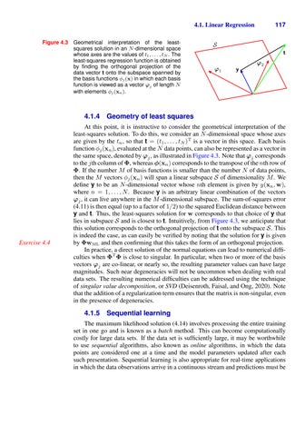
Geometrical interpretation of the leastsquares solution in an N -dimensional space whose axes are the values of t1 , . . . , tN . The least-squares regression function is obtained by finding the orthogonal projection of the data vector t onto the subspace spanned by the basis functions φj (x) in which each basis function is viewed as a vector ϕj of length N with elements φj (xn ).
S t ϕ1
y
ϕ2
4.1.4 Geometry of least squares
Exercise 4.4
At this point, it is instructive to consider the geometrical interpretation of the least-squares solution. To do this, we consider an N -dimensional space whose axes are given by the tn , so that t = (t1 , . . . , tN )T is a vector in this space. Each basis function φj (xn ), evaluated at the N data points, can also be represented as a vector in the same space, denoted by ϕj , as illustrated in Figure 4.3. Note that ϕj corresponds to the jth column of Φ, whereas φ(xn ) corresponds to the transpose of the nth row of Φ. If the number M of basis functions is smaller than the number N of data points, then the M vectors φj (xn ) will span a linear subspace S of dimensionality M . We define y to be an N -dimensional vector whose nth element is given by y(xn , w), where n = 1, . . . , N . Because y is an arbitrary linear combination of the vectors ϕj , it can live anywhere in the M -dimensional subspace. The sum-of-squares error (4.11) is then equal (up to a factor of 1/2) to the squared Euclidean distance between y and t. Thus, the least-squares solution for w corresponds to that choice of y that lies in subspace S and is closest to t. Intuitively, from Figure 4.3, we anticipate that this solution corresponds to the orthogonal projection of t onto the subspace S. This is indeed the case, as can easily be verified by noting that the solution for y is given by ΦwML and then confirming that this takes the form of an orthogonal projection. In practice, a direct solution of the normal equations can lead to numerical difficulties when ΦT Φ is close to singular. In particular, when two or more of the basis vectors ϕj are co-linear, or nearly so, the resulting parameter values can have large magnitudes. Such near degeneracies will not be uncommon when dealing with real data sets. The resulting numerical difficulties can be addressed using the technique of singular value decomposition, or SVD (Deisenroth, Faisal, and Ong, 2020). Note that the addition of a regularization term ensures that the matrix is non-singular, even in the presence of degeneracies.
4.1.5
Sequential learning
The maximum likelihood solution (4.14) involves processing the entire training set in one go and is known as a batch method. This can become computationally costly for large data sets. If the data set is sufficiently large, it may be worthwhile to use sequential algorithms, also known as online algorithms, in which the data points are considered one at a time and the model parameters updated after each such presentation. Sequential learning is also appropriate for real-time applications in which the data observations arrive in a continuous stream and predictions must be